
9
Analytical Expressions of FDS Transients
9.1. Introduction
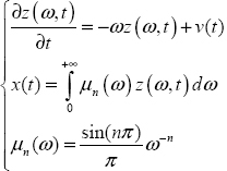
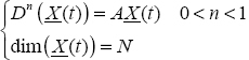
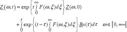
The determination of the analytical expression X(t) formulating the transients of the FDS:
is considered as a trivial problem because many researchers think that it has already been solved for several years with the initial condition X(0), where X(t) is the pseudo-state vector [MAT 96, BET 08]. Unfortunately, we have previously demonstrated that X(t) is unable to predict future system behavior, which must be replaced by the distributed state vector Z(ω,t), in the theoretical framework of the closed-loop representation. Moreover, it is generally admitted that X(t) expressions depend on the choice of the fractional derivative. We also demonstrated in Chapter 8 that it is a false problem and transients have a unique expression, which can be based on the distributed initial condition Z(ω, 0).
Therefore, the objective of this chapter is to express X(t), i.e. the free and forced responses of [9.1] using the distributed state Z(ω,t). Two solutions are proposed: the first solution is based on the Mittag-Leffler approach [MON 10, ORT 18] and the second solution is based on the new concept of distributed exponential, i.e. using all the potentialities of the infinite state approach. Moreover, beyond these theoretical expressions, another practical objective is to formulate computable solutions derived from these expressions.
Basically, the two theoretical solutions will be derived from Picard’s method; let us briefly recall its principle [KOR 68, POD 99].
This method is used to derive the solution of the nonlinear system:

The solution y(x) verifies the integral equation:
As y(x) on the right side is unknown, it must be replaced by iterative estimates yi(x).
At the first step, y0 (x) = y(x0).
Therefore
Then, at the second step, with estimate y1 (x), we can calculate:
Therefore, at iteration k, we obtain
This method makes it possible to obtain y(x) as:
This technique is essentially used in the nonlinear case [KOR 68], but obviously it can be used in the linear case.
9.2. Mittag-Leffler approach
9.2.1. Free response of the elementary FDS
Consider the elementary system
We have previously demonstrated that z(ω,0) is its initial condition, i.e. the initial condition of the associated fractional integrator ![]() with the closed-loop representation.
with the closed-loop representation.
Let us recall that:
The free response x0(t) of the integrator, with the initial condition z(ω,0), corresponds to v(t) = 0 .
Therefore
and
We look for the solution x(t) of system [9.8] using Picard’s method.
Basically, x(t) is the solution of the integral equation:
As x(t) on the right side is unknown, it must be replaced iteratively by x0 (t), x1(t) , …, xk (t).
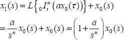
The first estimate is x0(t).
Therefore
and using the Laplace transform technique:
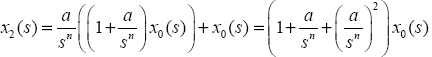
The second estimate x2(t) corresponds to
Therefore
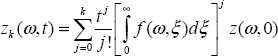
Consequently, at iteration k:
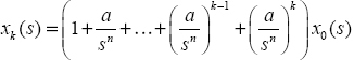
Therefore
Let us recall Appendix A.3:
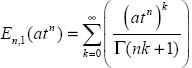
where ![]() is the Mittag-Leffler function defined as
is the Mittag-Leffler function defined as
Since
we obtain
Therefore
9.2.2. Free response of the N-derivative FDS
Consider
The initial condition of the integrators is Z(ω,0), and the free response X0 (t) of the integrators is defined as
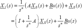
Basically, X(t) is the solution of the integral equation:
As noted previously, the first estimate is
which is expressed as X1 (s) with the Laplace transform technique:
Then
and
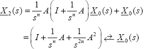
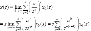
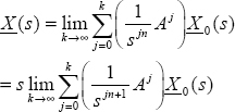
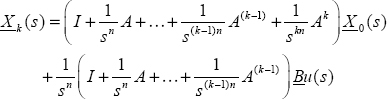
Therefore, at iteration k
and X(s) is the limit of this procedure:
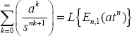
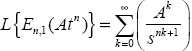
En,1 (Atn) is the matrix Mittag-Leffler function [MON 10] defined by the Laplace transform:
Then
and
where

is the matrix Mittag-Leffler function.
9.2.3. Complete solution of the N-derivative FDS
An excitation u(t) is introduced in the previous FDS, so
Z(ω, 0) is the initial condition of integrators ![]() and X0(t) is their free response [9.25].
and X0(t) is their free response [9.25].
Basically, X(t) is the solution of the integral equation:
As noted previously, the first estimate is:
Therefore
Then
Therefore
At iteration k, we obtain
Consequently, X (s) is the limit of this procedure:

Therefore
Let us define [MON 10]
Then
where
It would be possible to generalize this methodology to the non-commensurate order case. However, it would be of limited interest because even in the commensurate order case, practical computation of X(t) is difficult.
9.3. Distributed exponential approach
9.3.1. Introduction
The Mittag-Leffler approach is very popular among fractional calculus users [POD 99]. We demonstrated in the previous section that it can be adapted to the infinite state approach. Nevertheless, the expression
where
does not provide a straightforward access to the components of X(t) because it is based on a convolution integral.
Therefore, it seems more appropriate to determine another expression of X(t) using all the properties of the infinite state method.
9.3.2. Solution of 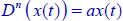 using frequency discretization
Consider the elementary system
which can be expressed with the internal distributed variable z(ω,t) :
Frequency discretization of this distributed differential system leads to (see Chapter 2):

Let us define
Equation [9.54] can be written as
with
Let us define

Thus, equation [9.53] can be expressed as
with
The differential equation [9.58] corresponds to the frequency discretization of the distributed differential system [9.52].
Let
Then, the solution of [9.58] with the initial condition [9.60] is expressed with the matrix exponential ![]() [KAI 80], i.e.
[KAI 80], i.e.
This technique is completely trivial in the context of integer order differential systems.
However, what is the limit of [9.61] if J ⟶ ∞, ωb ⟶ 0, ωh ⟶ ∞, Δω ⟶ 0?
This means that Z(t) ⟶ z(ω,t) and Z(0) ⟶ z(ω,0), which implies that ![]() becomes a matrix exponential of infinite dimension.
becomes a matrix exponential of infinite dimension.
Therefore, our objective is to express this limit.
9.3.3. Solution of  using a continuous approach
Consider again the distributed differential system
Using the equation defining x(t), we obtain
In fact, equation [9.63] is not correct because it is necessary to separate the frequency ω (of z(ω,t)) and the frequency ξ used in the calculus of the integral defining x(t).
Indeed, we must write
Consequently, there are two frequency variables ω and ξ.
It is possible to use only one variable ξ thanks to a mathematical trick.
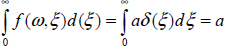
Consider the frequency Dirac impulse δ(ξ) [ZEM 65], defined as
Therefore, we can write
Let us define
Then

This means that the limit of the discretized system
is the distributed differential system
Therefore, ![]() is the continuous expression equivalent to
is the continuous expression equivalent to ![]() .
.
REMARK 1.– We can verify equation [9.70]. The discrete equivalent of ![]() ,
,
which corresponds to ![]() .
.
Note that two indexes j and k are necessary in order to separate ωj and ξk.
9.3.4. Solution of 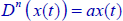 using Picard’s method
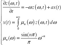
Consider the distributed differential system:
with the initial condition z(ω,0).
We use Picard’s method.
The solution z(ω,t) verifies the integral equation:

At the first iteration, z0 (ω,t) = z(ω,0)
Therefore, 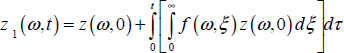
As ![]() does not depend on τ and ω
does not depend on τ and ω
we obtain
Then, at the second iteration:
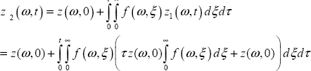
Thus
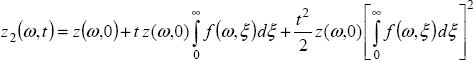
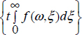
Consequently, at kth iteration:
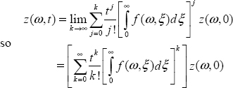
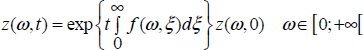
Let us define the distributed exponential as:
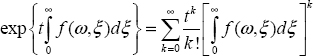
Thus, the solution of ![]() with the initial condition z (ω, 0) is expressed as:
with the initial condition z (ω, 0) is expressed as:
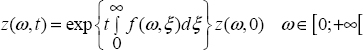
which is the continuous limit of ![]() .
.
REMARK 2.–
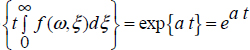
- 1) The elementary ODE

with the initial condition x(0) verifies the general solution:
x(t) = ea t x(0)
The distributed elementary ODE

with the initial condition z(ω, 0)
verifies the general solution:
Therefore, the distributed exponential exp
 is the generalization of the elementary exponential eat of the integer order case.
 - 2) Consider n = 1, then ω = 0 and μ1 (ξ) = δ(ξ)
so

and
Thus, exp
i.e. we recover the integer order case.
- 3) The main interest of the distributed exponential, in fact of its discretized version, is to provide a straightforward numerical solution expressed as:
for the free response of the elementary FDE
with the initial condition z(ω,0).
On the contrary, the Mittag-Leffler approach relies on a convolution
with ![]()
Obviously, the computation of this convolution is a complex operation.
Thus, the distributed exponential approach provides a tractable solution, generalization of the exponential in the integer order case.
9.3.5. Solution of 
Consider the non-commensurate order system:

Let Z (ω,t) be the vector of distributed states zi (ω,t) associated with each integrator ![]() i=1 to N. Then, system [9.80] is equivalent to
i=1 to N. Then, system [9.80] is equivalent to

where ![]() was defined in Chapter 7.
was defined in Chapter 7.
As in the one-derivative case, we can write
Note that
Therefore, we can define the matrix f(ω, ξ):
Then, system [9.81] can be expressed as
which is the generalization to the N -derivative case of
where ![]() .
.
Therefore, the distributed exponential exp ![]() is replaced by the distributed matrix exponential exp
is replaced by the distributed matrix exponential exp  , i.e.
is the solution of the non-commensurate order FDS ![]() with the initial condition Z(ω,0).
with the initial condition Z(ω,0).
Finally, we obtain X(t), the solution of [9.80] with:

9.3.6. Solution of 
Let us again consider the N -derivative FDS:
Z(ω,t) is the sum of the previous free response and the forced response due to the input u(t).
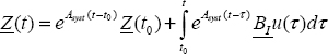
Therefore, as in the integer order case [KAI 80, ZAD 08]:

Thus, the complete solution is:
and the response X(t) of the system [9.80] is
9.4. Numerical computation of analytical transients
9.4.1. Introduction
The convolution of ![]() with
with ![]() is not an easy task; moreover, as En,1(atn) is not convergent for large values of t (see Chapter 7), computation of the free response with the Mittag-Leffler approach, even with an elementary fractional system, is a complex problem without practical interest.
is not an easy task; moreover, as En,1(atn) is not convergent for large values of t (see Chapter 7), computation of the free response with the Mittag-Leffler approach, even with an elementary fractional system, is a complex problem without practical interest.
On the contrary, computation of the free response based on the distributed exponential, in fact with its discretized expression, is straightforward, since it is the generalization of the integer order case which benefits many numerical tools [MOK 97].
However, computation of the forced response is not as simple as in the integer order case, i.e. a dedicated approach is necessary.
Two examples are proposed to highlight the interest of the discrete distributed exponential technique.
9.4.2. Computation of the forced response
Consider the elementary system:
Its frequency discretization leads to the equivalent integer order differential system:
with ![]() .
.
Therefore, the global solution of [9.94] with the discrete initial condition Z(t0) is:
Numerical computation of the free response is straightforward, as in the integer order case. In particular, we obtain the value of Z(t) directly, i.e. without recursive computation of intermediary values since t0.
On the contrary, there is a problem with the forced response.
Let t = kTe, where Te is the sampling period.
u(t) must be replaced between instants (k–1)Te and k Te by a constant value uk−1 (zero-holder [KAI 80, KRA 92]). Therefore, the convolution integral becomes:
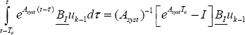
Let us recall that dim(Asyst) = (J + 1)(J + 1), where J + 1 is the number of frequency modes, with the constraint J >> 1. Moreover, as the frequency modes range from ωb to ωh, with ωh >> ωb, the matrix Asyst is ill-conditioned and cannot be inverted [FRA 68, DEN 69, MAR 93]. Therefore, it is necessary to numerically compute the convolution integral.

Therefore, 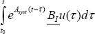 corresponds to the recursive equation:
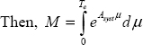
M is precomputed thanks to a numerical integration algorithm [HAR 98, NOU 91].
For example, we can compute M using the simplest elementary algorithm:
In order to appreciate the accuracy of this technique, we must compute the forced response ![]() of
of ![]() with u(t) = UH(t) and compare it to the reference output xref(t) = U(1−En,1(–atn)) (see Appendix A.3).
with u(t) = UH(t) and compare it to the reference output xref(t) = U(1−En,1(–atn)) (see Appendix A.3).
The simulation is performed with
Figure 9.1 presents the computation error ![]() for different values of Te.
for different values of Te.

Figure 9.1. Computation error. For a color version of the figures in this chapter see www.iste.co.uk/trigeassou/analysis1.zip
This error is very low for Te =10−3 s and Te =10−2 s . As expected, it is more important for Te = 0.1s, but nevertheless acceptable.
9.4.3. Step response of a three-derivative FDS
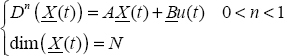
Consider the non-commensurate order FDS:
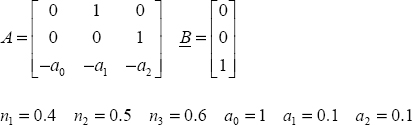
![]() correspond to:
correspond to:

X(t) is computed with the recursive equation:
G is precomputed with the previous integration technique (I = 2000).
The graphs of x1(t), x2 (t) and x3(t) are plotted in Figure 9.2.

Figure 9.2. Step responses of pseudo-state variables
Note that dim (Asyst ) = (153) (153) , which is obviously a large value for an integer order system.
Thus, this example perfectly illustrates the numerical robustness of the discrete distributed exponential algorithm.