
10
Infinite State and Fractional Differentiation of Functions
10.1. Introduction
Fractional calculus has concerned the calculation of fractional integrals and derivatives for any kind of functions for a long time (see [OLD 72, MIL 93] and the references therein). Of course, integration of FDEs has also been an important issue, stimulated by physical and engineering applications [SAM 87, POD 99].
In the previous chapters, the infinite state approach was applied to the modeling and analysis of FDEs. In fact, this methodology also applies to other domains of fractional calculus, and particularly to the calculation of the fractional derivative of a function g(t), i.e. to ![]() . This derivative depends on the differentiation technique used: Riemann–Liouville, Caputo or Grünwald–Letnikov.
. This derivative depends on the differentiation technique used: Riemann–Liouville, Caputo or Grünwald–Letnikov.
Let us consider the calculation of ![]() with the Caputo derivative. In the first step, we demonstrate that the calculation of the Caputo derivative on an infinite interval
with the Caputo derivative. In the first step, we demonstrate that the calculation of the Caputo derivative on an infinite interval ![]() makes it possible to express the fractional derivative of the function g(t). In the second step, we analyze the calculation of the Caputo derivative on a truncated interval
makes it possible to express the fractional derivative of the function g(t). In the second step, we analyze the calculation of the Caputo derivative on a truncated interval ![]() and the initial condition problem arising at t = t0. Thus, we demonstrate that knowledge of these initial conditions makes it possible to correct the calculation on a truncated interval and thus to recover
and the initial condition problem arising at t = t0. Thus, we demonstrate that knowledge of these initial conditions makes it possible to correct the calculation on a truncated interval and thus to recover ![]() [TRI 11d, TRI 11e]. We consider some generic functions and formulate their fractional derivatives and the corresponding initial conditions.
[TRI 11d, TRI 11e]. We consider some generic functions and formulate their fractional derivatives and the corresponding initial conditions.
Moreover, we demonstrate that the implicit derivative is also able to express the fractional derivative ![]() . Finally, numerical simulations are used to illustrate previous results for the particular case of the sine function.
. Finally, numerical simulations are used to illustrate previous results for the particular case of the sine function.
10.2. Calculation of the Caputo derivative
Let us consider a function g(t) defined for ![]() , and we propose to analytically determine its fractional derivative
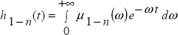
, and we propose to analytically determine its fractional derivative ![]() for 0 < n < 1. Let us recall (Chapter 8) that the Caputo derivative calculated since t = −∞ is equal to the fractional derivative of f(t) because all the possible transients have vanished, so
for 0 < n < 1. Let us recall (Chapter 8) that the Caputo derivative calculated since t = −∞ is equal to the fractional derivative of f(t) because all the possible transients have vanished, so
where ![]() is the theoretical fractional derivative of g(t).
is the theoretical fractional derivative of g(t).
Let us recall that the Caputo derivative is defined as:
i.e. the Caputo derivative is the Riemann–Liouville integral, with order 1 – n , of the integer order derivative ![]() .
.
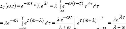
Let zc(ω, t) be the distributed state variable of the integrator ![]() . Thus, zc(ω, t) and
. Thus, zc(ω, t) and ![]() are solutions of the distributed differential system:
are solutions of the distributed differential system:
Equation [10.3] means that zc(ω, t) is the convolution of ![]() with the impulse response hω(t) of a first-order elementary system
with the impulse response hω(t) of a first-order elementary system ![]() , where
, where
Therefore
With zc(ω, t), we finally obtain the fractional derivative as the weighted integral of all the frequency components, using equation [10.4].
Then, we apply this methodology to some generic functions (see [POD 99]).
10.2.1. Fractional derivative of the Heaviside function
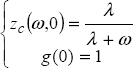
Consider the Heaviside function:
We note that
Therefore, using equation [10.3]:
Then, using equation [10.4]:
As
we can write
Let us recall that
Therefore
and
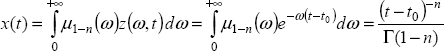
10.2.2. Fractional derivative of the power function
Let us define the power function:
Then
Consider the variable change:
Therefore

Using equation [10.3]
and with equation [10.4]
As
we obtain
Using the convolution lemma (Appendix A.10):
We finally obtain
10.2.3. Fractional derivative of the exponential function
Consider the exponential function:
Then
Using equation [10.3]
Therefore, with equation [10.4]
Let us recall that
Therefore, with s = λ, we obtain
and
10.2.4. Fractional derivative of the sine function
Consider the sine function
and its derivative
As

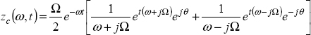
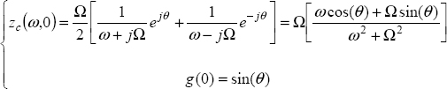
Equation [10.3] can be written as
Therefore, this equation corresponds to

and using equation [10.40]:
As (equation [10.32]),
we obtain, with x = j Ω:
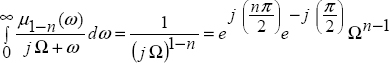
Finally

which yields:
10.3. Initial conditions of the Caputo derivative
We have previously defined the initial conditions of the Caputo derivative in the context of FDS transients. Our objective is to revisit these definitions, in the context of the calculation of the Caputo derivative applied to a function g(t).
In order to express the fractional derivative ![]() , we have calculated the Caputo derivative on an infinite interval
, we have calculated the Caputo derivative on an infinite interval ![]() . Practically, the derivative is calculated on a truncated interval
. Practically, the derivative is calculated on a truncated interval ![]() .
.
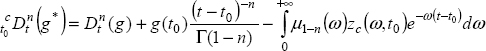
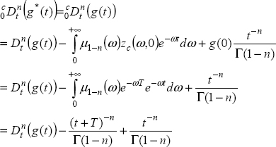
Consequently, the function g(t) is truncated. Let g*(t) be this new function:
Therefore, we calculate

On the other hand
As
We obtain
Then:
REMARK 1.– Let ![]() , and define
, and define
Then
thus
Therefore, [10.49] is expressed as
We have previously defined [10.1]:
Therefore, using the convolution relation (see Chapter 6), we can write

where ![]() is the value of the distributed variable zc(ω, t) of the integrator
is the value of the distributed variable zc(ω, t) of the integrator ![]() at instant t0 (when the integrator acts since t = –∞).
at instant t0 (when the integrator acts since t = –∞).
Note that ![]()
so equation [10.51] can be written as
Similarly, [10.52] can be written as

Equaling these two expressions of ![]() , we obtain:
, we obtain:
The two “initial conditions” are g(t0) and zc(ω, t0).
The distributed variable zc(ω, t0) is a true initial condition, corresponding to the distributed variable zc(ω, t) at t = t0 of the integrator ![]() , acting since t = −∞.
, acting since t = −∞.
On the contrary, g(t0) is a pseudo-initial condition [ORT 11]: it corresponds to the jump of the truncated function g*(t) from g*(t) = 0 for t < t0 to g(t) at t = t0. The derivative of this jump provides the Dirac g(t0)δ(t − t0).
Moreover, note that
and

Therefore
This means that the Caputo derivative, calculated since any instant t0 , tends asymptotically towards the fractional derivative of g(t), with a long memory transient.
10.4. Transients of fractional derivatives
10.4.1. Introduction
We have demonstrated that the Caputo derivative of the truncated function ![]() converges asymptotically towards the exact value
converges asymptotically towards the exact value ![]() with a long memory transient.
with a long memory transient.
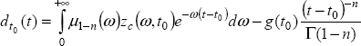
This convergence is characterized by a transient ![]() depending on the “initial conditions” g(t0) and zc(ω,t0).
depending on the “initial conditions” g(t0) and zc(ω,t0).
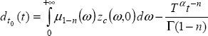
This transient is defined as
i.e.
Let us define these “initial conditions” for the previous generic functions; in order to simplify calculations, let t0 = 0 .
10.4.2. Heaviside function
Consider g(t) = H(t + T) with T > 0 . Then
We have previously calculated
Therefore
and
Then
Thus
10.4.3. Power function
Consider ![]() with T > 0 and its truncation
with T > 0 and its truncation ![]()
We have previously calculated
and

Therefore
10.4.4. Exponential function
Consider ![]() and its truncation
and its truncation ![]()
We have previously calculated
Therefore
Consequently

10.4.5. Sine function
Consider ![]() and its truncation
and its truncation ![]()
We have previously calculated
Therefore
Consider the particular value θ = 0, and then
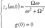
Therefore
10.5. Calculation of fractional derivatives with the implicit derivative
10.5.1. Introduction
We have demonstrated the interest of the infinite state approach for the calculation of the fractional derivative of a function g(t), i.e. the distributed model zc(ω,t) of the fractional integrator ![]() makes it possible to calculate this fractional derivative using the Caputo derivative definition.
makes it possible to calculate this fractional derivative using the Caputo derivative definition.
Similarly, we can calculate fractional derivatives with the distributed model associated with the Riemann–Liouville derivative.
More surprisingly, we can also use the implicit derivative. Of course, it is not possible to use the closed-loop formulation of the implicit derivative.
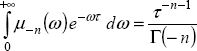
Let us recall that the analytical expression of this derivative (see Chapter 8) corresponds to:
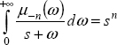
where
As ![]() we obtain, for α = −n
we obtain, for α = −n
Let zI(ω,t) be the distributed variable associated with the implicit derivative:

10.5.2. Fractional derivative of the Heaviside function
Consider the Heaviside function g(t) = H(t + T).
Then
Therefore
and
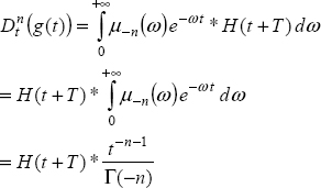
Thus
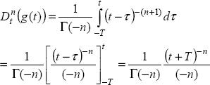
As Γ(x + 1) = xΓ(x) (see Appendix A.1.4), we obtain Γ(1 − n) = −nΓ(−n).
Therefore
10.5.3. Fractional derivative of the power function
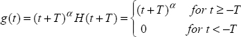
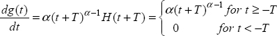
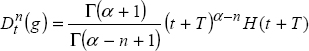
Consider the power function g(t) = (t + T)αH(t + T).
Then
Consider the variable change τ = (t + T)
Therefore
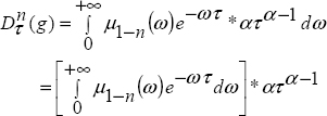
and
Then

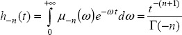
As
we obtain
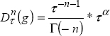
Using the convolution lemma (Appendix A.10):
Finally
10.5.4. Fractional derivative of the exponential function
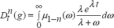
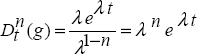
Consider the exponential function g(t) = eλt.
Therefore
and
Using the results of section 10.2.3, we obtain
Therefore

As
With s = λ, we obtain
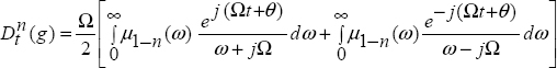
10.5.5. Fractional derivative of the sine function
Consider the sine function 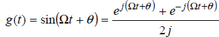 .
.
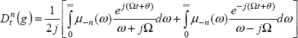
Therefore
and

Then
As

where ![]() and
and ![]() , we obtain
, we obtain

Therefore
10.5.6. Conclusion
Obviously, we have obtained the same results for ![]() using either the Caputo derivative or the implicit derivative.
using either the Caputo derivative or the implicit derivative.
As discussed previously, it would be straightforward to define the initial conditions of the implicit derivative and the corresponding transients of ![]() , where g*(t) is the truncation of function g(t).
, where g*(t) is the truncation of function g(t).
10.6. Numerical validation of Caputo derivative transients
10.6.1. Introduction
Previous results are essentially theoretical. They do not provide a practical understanding on the computation of the Caputo derivative and particularly of transients caused by initial conditions. Thus, we hereafter illustrate this problem with the sine function.
The objective is to compare the exact fractional derivative ![]() and the Caputo derivative
and the Caputo derivative ![]() computed since t = 0. Thanks to the theoretical values of the corresponding initial conditions, theoretical transients can be computed and compared to the observed ones.
computed since t = 0. Thanks to the theoretical values of the corresponding initial conditions, theoretical transients can be computed and compared to the observed ones.
Let us recall:
Sine function: g(t) = sin(Ωt + θ).
Fractional derivative: ![]() sin
sin  .
.
Computed Caputo derivative: ![]()
Transients:

Let us note that the term related to g(t0) is a false problem: it represents the amplitude of the jump caused by the truncation of g(t). The corresponding transient can be easily removed by the computation of ![]() . Thus, we will only consider the influence of the distributed initial condition zC(ω,0) .
. Thus, we will only consider the influence of the distributed initial condition zC(ω,0) .
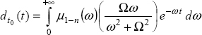
We have demonstrated: ![]() .
.
The corresponding transient is defined as:
It is compared to
10.6.2. Simulation results
Numerical simulations are performed with:
Riemann–Liouville integration: 1–n = 0.5
Sine function: ![]()
Figure 10.1 presents the graphs of ![]() and
and ![]() for
for ![]() .
.

Figure 10.1. Sine function fractional derivatives. For a color version of the figures in this chapter, see www.iste.co.uk/trigeassou/analysis1.zip
An obvious difference exists between the exact and computed fractional derivatives. It is also obvious that a very long transient is necessary for convergence of the computed derivative.
Figure 10.2 presents the variation of zC (ω,0) for different values of θ.
These graphs highlight the influence of the lower frequency modes, i.e. the long memory behavior of d(t) .
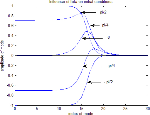
Figure 10.2. Sine function truncation and corresponding initial conditions
Figure 10.3 exhibits the graphs of d(t) and dth(t) for the corresponding values of θ. These graphs are identical: this means that equation [10.106] allows a perfect prediction of transients. The influence of θ is maximum for ![]() . On the contrary, fast convergence is provided by θ=0, as the lower frequency modes are close to 0.
. On the contrary, fast convergence is provided by θ=0, as the lower frequency modes are close to 0.

Figure 10.3. Sine function truncation and corresponding transients
A.10. Appendix: convolution lemma
The objective is to express the convolution product
Let

and
Recall that
Then
AS
we obtain