
5
Modeling of Physical Systems with Fractional Models: an Illustrative Example
5.1. Introduction
In Chapter 4, we demonstrated that the diffusive heat transfer interface, governed by a partial differentiation equation, can be modeled by a fractional transfer function, independently of the physics of the interface. More generally, this means that the dynamical behavior of a physical system can be approximated by a differential mathematical model (linear or nonlinear) with integer order derivatives or fractional order ones. The heat transfer example has justified the interest of fractional modeling for systems governed by a diffusive equation, i.e. with dynamics characterized by long memory behavior. We also demonstrated that the structure cannot be chosen arbitrarily; on the contrary, these models must satisfy structural constraints, in particular for identification purposes.
More generally, it is necessary to remember some basic principles for modeling and identification related to the system theory. In particular, it is important to differentiate between modeling concepts such as the knowledge model, the behavior model or the black box model and the intermediate category called the gray box model [TUL 93, WAL 97, TRI 01].
In order to specify these essential notions, we consider an illustrative example, the induction motor [ALG 95]. During the last decades, it has gradually replaced the DC motor in variable speed applications, mainly for rail traction [BOS 86, HUS 09]. The induction motor is characterized by simple manufacturing and robustness, compared to the DC motor. On the contrary, its modeling is more complex, particularly for squirrel cage motors, where induced currents are governed by a diffusion equation. Using fractional representation, modeling of this motor can be improved by the association of integer and fractional order differential systems [BEN 04, CAN 05a].
The resulting model is called fractional Park’s model [JAL 13] which is a perfect justification of the non-commensurate order concept with a global model composed of an integer order part and a fractional one with different orders. Therefore, we present the different steps of the modeling of the induction motor and of the identification of its fractional Park’s model in order to illustrate the modeling concepts.
5.2. Modeling with mathematical models: some basic principles
Mathematical models used for the modeling of either physical, chemical or biological process are usually ordinary differential equations, partial differential equations and/or FDEs.
Indeed, a physical process is generally governed by a set of differential equations or partial differential equations, linear or nonlinear, stationary or not. This model is generally complex, based on elementary physical laws; it requires the intervention of an expert of the process. This model is too complex to be used for the design of a control law. It is called the knowledge model and its main use is for numerical simulation of the physical system [EYK 74, WAL 97].
The knowledge model is used to define a low complexity model called the black box model [LAN 89]. This model known as the behavior model is intended to reproduce the dynamics of the original system with low-order differential equations or difference equations. Therefore, the black box model is only a mathematical model not related to the physics of the actual system. Nevertheless, it is sometimes required that this model be related to some parts of the original system. Consequently, this model is called the gray box model; it is composed of differential equations whose parameters can be related to physics [TUL 93, TRI 01].
The black box or gray box model can be provided by mathematical approximation; however, it is difficult to give a relevant value to its parameters. Thus, a convenient way to obtain these models is to use identification techniques [RIC 71, TRI 88, RIC 91]. The model is provided by the minimization of a quadratic criterion of the error between experimental data and a simulation of the system model. Data measurements are provided by a digital data acquisition system with sampling period Te associated with data anti-aliasing filters excluding dynamics beyond the Shannon frequency. Moreover, the excitation of the system is provided by an input sequence in a frequency band {ωb,ωh} , where ωh is imposed by the choice of the sampling period Te [LJU 87]. Obviously, thanks to the frequency band {ωb,ωh} high frequency modes (and low frequency ones) of fractional models (and also of integer order models) can be neglected. Finally, it is important to note that data measurements are disturbed by stochastic noise which causes errors in parameter estimates and model structure.
For control purposes, black box models such as Z -transfer functions are preferred because they are well suited to controller design techniques [LAN 89].
The identification methodology is more complex for gray box models which have to partially respect the physics of the considered system. Thus, it is necessary to use physical knowledge to discriminate identified models, associated with low quadratic values, which provide biased estimations of parameters and model structure. This is a difficult issue for any type of model and in particular for fractional models [TRI 01].
5.3. Modeling of the induction motor
5.3.1. Construction of the induction motor
The induction motor is an electrical machine composed of three-phase windings at the stator and of a squirrel cage rotor. The squirrel cage is so called because it is composed of short-circuited conductor bars (for more details, see [ALG 95]).
5.3.2. Principle of operation
The three windings of the stator are fed by three-phase currents {ia(t),ib(t),ic(t)}. These currents set up a rotating magnetic field of constant amplitude; the magnetic rotating speed Ωs is imposed by frequency F of the currents, with Ωs = 2πF .
The rotating magnetic field induces three-phase currents in the short-circuited rotor bars. In turn, rotor currents produce a magnetic field that revolves at the same speed as the stator field.
The interaction between the two fields produces a torque. According to Lenz’s law, this torque makes the rotor to move so as to reduce the relative speed between the stator flux speed (Ωs) and the rotor flux speed (ΩR). Note that ΩR cannot be equal to Ωs because there will be no induced rotor currents and consequently no torque.
The relative speed Ωs − ΩR is characterized by its normalized value s, called the slip such as
At full load, slip is equal to only a few percent, for example 5%. Torque is proportional to slip as s → 0 and decreases as s → 1 . However, the starting torque (s = 1) is high enough to move heavy loads, which is a supplementary interest of the induction motor.
Reciprocally, its main drawback has been for a long time the impossibility of performing variable speed, because Ωs is imposed by frequency F.
Fortunately, it is now easy to realize variable frequency electrical supplies, so as to perform variable speed operation [BOS 86].
5.3.3. Induction motor knowledge model
An electrical model is required by many applications, such as induction motor design. Electrical engineers have proposed models associating magnetic fields with three-phase currents, such as in the synchronous machine. It is easy to calculate the rotating field created by the stator. On the contrary, for the rotor, it is a more complex issue because induced currents in rotor bars are governed by a diffusive phenomenon.
Consider the rectangular bar of Figure 5.1.
At low frequencies, currents have a density ![]() which is uniform everywhere over the entire cross-sectional area. If the frequency is high enough, current density tends to be higher at the surface of the bar. The higher the frequency, the greater the tendency for this effect to occur. This phenomenon is called the skin effect in rotor bars or frequency effects [KAB 97, JOO 86].
which is uniform everywhere over the entire cross-sectional area. If the frequency is high enough, current density tends to be higher at the surface of the bar. The higher the frequency, the greater the tendency for this effect to occur. This phenomenon is called the skin effect in rotor bars or frequency effects [KAB 97, JOO 86].
Let us consider the rectangular massive conductor of Figure 5.1.
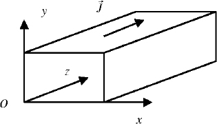
Figure 5.1. Rectangular rotor bar
The transients of the skin effect phenomenon are related to the partial differential diffusive equation:
where
is the current density.
Modeling of the diffusive phenomenon is classical. With heat transfer, a space discretization technique [FAR 82] is often used (see Chapter 5 volume 2). It is a more complex issue with rotor bars. A more sophisticated approach, the finite element method [COU 85, NOU 91], must be used with the induction machine. The reader can refer to research works reported in [KHA 01, CAN 05b]. This simulation technique provides very accurate results, in particular for the design of rotor bars.
Its essential drawback is large computation time. However, these simulations have demonstrated the fractional behavior of currents in rotor bars.
Frequency analysis of induced currents in rotor bars [KHA 01] provides frequency response graphs (see Figure 5.2) which are similar to the theoretical heat transfer ones (see Chapter 4).

Figure 5.2. Induced current frequency responses versus rotor bar cross-sections
5.3.4. Park’s model
The knowledge model is perfectly adapted to the design of electrical machines, such as optimal design of cross-sectional rotor bars, but it is unable to help the electrical engineer for the design of variable speed control algorithms.
For this purpose, engineers use Park’s model based on a limited number of electrical components, such as resistors and inductors. Therefore, it corresponds to the model-type called the gray box model.
Important simplifying assumptions are necessary to derive this model [PAR 29, POL 87]. In particular, induced currents are assumed to be uniform in rotor bars.
Voltages are defined as {usa,usb,usc} for the stator and {uRa,uRb,uRc} for the rotor. They are related to currents i and flux ϕ by the equations


The three-phase model ([5.4], [5.5]) can be simplified by the application of Park’s transformation:
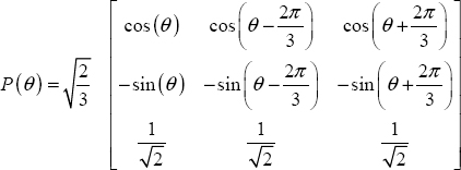
This transformation establishes an equivalence between a three-phase representation and a ![]() reference frame [PAR 29]. In practice, the complex notation is used to simplify equations:
reference frame [PAR 29]. In practice, the complex notation is used to simplify equations:
where xd and xq are components corresponding to a ![]() reference frame axis.
reference frame axis.
For example, with the reference frame related to the rotor, the model of the induction motor is:
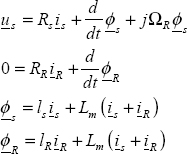
where ΩR is the rotor speed, Rs and RR are the stator and rotor resistors, ls and lR are the stator and rotor leakage inductors and Lm is the magnetizing inductor.
The torque can be expressed as:
The conventional electrical diagram of Park’s model is presented in Figure 5.3.
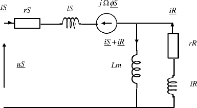
Figure 5.3. Park’s model
5.3.5. Fractional Park’s model
For the variable speed operation, the variable frequency electrical supply is based on a pulse width modulation (PWM) technique [BOS 86]. Therefore, supply voltage is characterized by a large number of harmonics and induced rotor currents include high frequency components. Consequently, the skin effect is present in rotor bars and the elementary Park’s model is inappropriate to correctly represent transients in rotor bars.
A direct improvement is to discretize currents in rotor bars according to Figure 5.4.
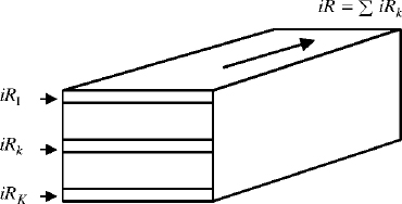
Figure 5.4. Discretization of iR in rotor bars
If we define the electrical model of slice k as {RR,k,lR,k}, the elementary diagram {RR,lR} of Figure 5.3 can be replaced by a ladder network (see Figure 5.5).
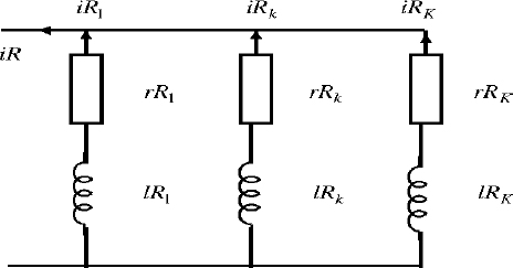
Figure 5.5. Rotor ladder network
However, it is not possible to define the values of {RR,k,lR,k} for k = 1 to K.
An attempt has been made to estimate these values using an identification technique: practically, it is limited to K = 2 [KAB 97].
In fact, each branch of the ladder corresponds to a frequency mode ωk which can be interpreted as the frequency mode of a frequency distributed fractional impedance:
Therefore, according to the previous analysis of the heat transfer diffusive process (Chapter 4), we can use for ZR(s) the one-derivative black box model:
or the two-derivative one:
The resulting model [JAL 10, JAL 12] is presented in Figure 5.6.
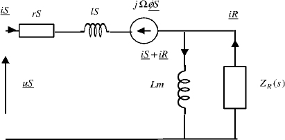
Figure 5.6. Fractional Park’s model
Note that this global model associates an integer order gray box model with a fractional black box one.
5.4. Identification of fractional Park’s model
5.4.1. Simplified model
The fractional Park’s model can be identified from measurements provided by normal operation. However, data measurements are usually disturbed by various noises so confident estimation of all the parameters of the fractional model cannot be performed.
Thus, electrical engineers have proposed an alternative to this issue called the standstill operation. Therefore, rotor speed is equal to zero and a special connection of stator windings is used [LIN 01a]. Moreover, stator is fed by a rectangular-type electrical supply [BOS 86]. Therefore, data measurements are us (t) and is (t), and the fractional Park’s model is presented in Figure 5.7.
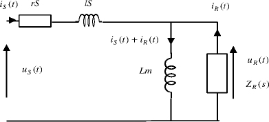
Figure 5.7. Simplified fractional Park’s model
If ![]() the differential system corresponds to
the differential system corresponds to
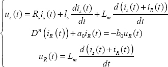
REMARK 1.– ls is assumed to be equal to zero in order to simplify the identification procedure, either for the usual Park’s model or the fractional one.
5.4.2. Identification algorithm
The identification algorithm used to perform parameter estimation of the fractional Park’s model is known as the model method [RIC 71] (Figure 5.8) or the output error method [LJU 87].
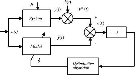
Figure 5.8. Output error method
The system is characterized by its model structure f and its parameters θ.
Its exact output y(t) depends on the model f, its parameters θ and excitation u(t).
Therefore,
The model y(t) = f(θ,u(t)) is generally a nonlinear differential system. Data measurements are u(t) and y*(t) = y(t) + b(t), where b(t) is a stochastic disturbance.
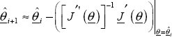
Assuming that the model structure is known, ![]() represents the simulation of the model based on the knowledge of u(t) and of
represents the simulation of the model based on the knowledge of u(t) and of ![]() (prior estimation θ).
(prior estimation θ).
Therefore,
![]() and
and ![]() are available at sampling instants t = kTe, so
are available at sampling instants t = kTe, so ![]() and
and ![]() .
.
We can define the simulation error as
and the quadratic criterion
The objective of the identification procedure is to estimate θ by minimizing criterion J.
5.4.3. Nonlinear optimization
Criterion J is a nonlinear function of ![]()
The objective is to obtain θopt which is the optimal estimation of θ. Any value θmin minimizing J [KOR 68, HIM 72] is defined by ![]() and
and 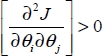 .
.
However, this condition is not sufficient to define θopt (global optimum) because several values of θmin (secondary optimum) can occur [RIC 71, WAL 97].
Therefore, we obtain
There are many nonlinear optimization techniques available to perform the estimation of θopt [BOU 67, HIM 72].
All of these optimization techniques are random search techniques, depending on a starting value θinit.
In practice, we have used a search technique derived from the gradient technique [TRI 88, TRI 01].
The output error method requires an important assumption: θinit should be in the vicinity of θopt . θinit can be derived from some physical knowledge of θ or provided by another identification algorithm, such as the least-squares method [MEN 73, NOR 86, LJU 87, COI 01]. An improved methodology is derived to initialize parameter estimation of fractional order models [KHA 15a, KHA 15b].
The optimum θopt corresponds to
where the partial derivatives ![]() measure the sensitivity of simulated output
measure the sensitivity of simulated output ![]() to the variations of
to the variations of ![]()
Let us define
Therefore,
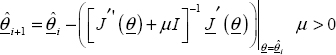
Several iterative techniques are available to reach θopt from prior estimation ![]()
- – Gradient method (or steepest descent method) [HIM 72]:
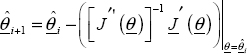
- – Gauss–Newton method [HIM 72]:
- – Levenberg–Marquardt method [MAR 63]:
The stability of the gradient method depends on the parameter λ (if λ ≈ 0, stability is ensured, but convergence is very slow).
If ![]() is close to θopt, criterion J is a quadratic function of θ and the optimum θopt is theoretically obtained in one iteration with the Gauss–Newton algorithm; otherwise, divergence of this algorithm can occur.
is close to θopt, criterion J is a quadratic function of θ and the optimum θopt is theoretically obtained in one iteration with the Gauss–Newton algorithm; otherwise, divergence of this algorithm can occur.
Levenberg–Marquardt is a compromise between the two previous algorithms. If ![]() is far from θopt, we must choose a large value of μ, thus
is far from θopt, we must choose a large value of μ, thus
Therefore, the algorithm behaves like the gradient one and convergence is slow but ensured.
On the contrary, if μ → 0
Therefore, the algorithm behaves like the Gauss–Newton one and fast convergence is ensured.
Of course, the value of μ should be automatically monitored to ensure convergence [MAR 63, TRI 01].
5.4.4. Simulation of  and
and 
![]() is a simulation of
is a simulation of ![]() i.e. a simulation of a differential system, which is composed of an integer order part and a fractional order one with Park’s model.
i.e. a simulation of a differential system, which is composed of an integer order part and a fractional order one with Park’s model. ![]() should be resimulated at each iteration i of the nonlinear optimization algorithm.
should be resimulated at each iteration i of the nonlinear optimization algorithm.
σk results also of the simulation of a differential system (see [TRI 01]); it should also be simulated at each iteration i.
As fractional order n (or n1) is unknown, it has to be estimated [VIC 13]. Derivation of σk related to n is a complex task [POI 04]. Fortunately, ![]() can be approximated by
can be approximated by
Note that Δn can be chosen a priori [DJA 08, JAL 12] because ![]() is necessarily in the interval [0,1].
is necessarily in the interval [0,1].
The approximate computation of ![]() is also possible, but it is more complex because Δθj must be adapted at each iteration [HIM 72].
is also possible, but it is more complex because Δθj must be adapted at each iteration [HIM 72].
5.4.5. Comments
The main advantage of the output error method is related to its nice statistical properties. If the noise b(t) disturbing y*(t) is zero mean and as ![]() does not depend on b(t), then θopt can be considered as a confident estimation [WAL 97, TRI 01] of θ, i.e.
does not depend on b(t), then θopt can be considered as a confident estimation [WAL 97, TRI 01] of θ, i.e. ![]() (number of data points).
(number of data points).
Note that θMC (estimation of θ provided by the least-squares method) is a biased estimate of θ, i.e. ![]()
Δθ is called an estimation bias; it depends on the statistical characteristics of b(t) [EYK 74, LJU 87].
Therefore, θMC is not a confident estimation of θ, but it can be used to initialize a nonlinear optimization technique: θinit = θMC.
Note that it is impossible to know the exact structure of a system model. Therefore, modeling errors are always present, which can be interpreted as a disturbing noise by the identification algorithm.
Unfortunately, this modeling noise is not zero mean and θopt is necessarily biased by modeling errors.
Globally, in spite of modeling errors, the output error identification algorithm is a relevant technique.
However, simulation of model and sensitivity functions are difficult to implement with complex nonlinear differential systems. Moreover, it is essential to note that it requires large computation time if we compare it to the more simple least-squares techniques [LJU 87].
5.4.6. Application to the identification of fractional Park’s model
Data measurements us(t) and is(t) (we present only the beginning of data files) are shown in Figures 5.9 and 5.10.
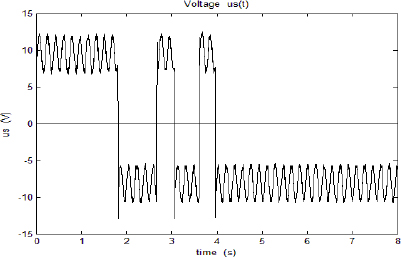
Figure 5.9. uS(t) voltage
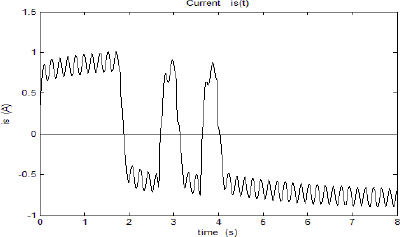
Figure 5.10. iS(t) current
us(t) is a PMW voltage modulated by a pseudo-random binary sequence. The sampling period Te is equal to 3.6 ms and K = 9000 .
Three model structures are identified and compared:
- – H(s) usual Park’s model;
- – Hn(s) fractional Park’s model with ZR(s)=Zn(s) ;
- – Hn1 ,n2(s) fractional Park’s model with ZR (s)=Zn1 ,n2(s) .
The corresponding results are presented in Tables 5.1–5.3.
Table 5.1. Parameter estimations H(s)
| RS(Ω) | Lm(H) | RR(Ω) | lR(H) | J |
| 9.96 | 0.40 | 4.01 | 0.08 | 9.08 |
Table 5.3. Parameter estimations Hn1,n2(s)
| RS(Ω) | Lm(H ) | a0 | a1 | b0 | b1 | n1 | J |
| 9.93 | 0.40 | 42.70 | 1.93 | 10.24 | 0.25 | 0.48 | 7.88 |
Compared to usual Park’s model, there is an improvement with the two fractional models corresponding to a decrease in criterion values.
Moreover, Hn1,n2(s) provides a better approximation of the induction motor than Hn(s) .
Note that the values of Rs and Lm are approximately the same for the three models.
Hn1,n2(s) is more complex than Hn(s) , accompanied by a low decrease of J: it would seem reasonable to prefer Hn(s) instead of Hn1,n2(s) , in contrast to the conclusions of Chapter 4.
In fact, a discrimination technique presented in [JAL 13] demonstrates that Hn(s) is unable to provide a confident behavior model in comparison with Hn1,n2(s), in accordance with the conclusions of Chapter 4.
We can conclude that fractional gray box modeling and identification are relevant techniques, but they must be carried out with much care using all the possibilities provided by physics, statistics and advanced identification techniques.