
2
Frequency Approach to the Synthesis of the Fractional Integrator
2.1. Introduction
In Chapter 1, we defined fractional integration as the key tool for modeling and simulation of FDEs. Unfortunately, the definition of Riemann–Liouville integration
where
does not provide a suitable technique for the numerical simulation of fractional integration, which is not a classical integral, but in fact a convolution integral.
Therefore, in the first step, we relate this operation to a frequency approach based on the Laplace transform of hn(t), thus:
In the second step (Chapter 6), we will relate fractional integration to a time approach, called the infinite state approach, moreover demonstrating that these two approaches are equivalent and complementary.
The synthesis of the fractional integrator thanks to a frequency methodology is in fact based on Oustaloup’s technique [OUS 00] for the synthesis of the fractional differentiator Dn(s) = sn.
Therefore, in this chapter, we present a frequency approximation of In(s) which will be used to derive a modal formulation, basis of the numerical integration algorithm and of the fractional integrator state variables.
2.2. Frequency synthesis of the fractional derivator
The first researcher who proposed a constant phase template, i.e.
in order to robustify the feedback closed-loop with respect to open-loop static gain variations was Bode [BOD 45]. This idea was reused by Manabe [MAN 60]. However, it is really Oustaloup, independently of these two pioneers, who formalized this principle and defined the concepts of the fractional template in his famous monographs [OUS 81, OUS 83, OUS 91].
The concept of fractional differentiation sn is fundamental to the definition of the corresponding robust controller. In other monographs [OUS 95a] and [OUS 95b], Oustaloup has proposed a complete methodology for the synthesis of the fractional differentiator in a frequency band. This principle has been reused by numerous researchers [RAY 97, VIN 00, POD 02b, DAS 11], and we can say that it really marks the beginning of a realistic use of fractional calculus in the automatic control domain, and more generally in various engineering domains.
Our frequency approach is completely based on this methodology, so we have to summarize it thereafter.
The objective is to provide a practical realization of Dn(s) = sn (with 0 < n < 1) in a frequency band ![]() . Let
. Let ![]() be the ideal derivator in the band
be the ideal derivator in the band ![]() . It is defined by the relation:
. It is defined by the relation:
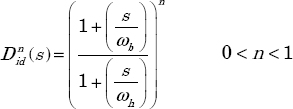
In the frequency domain, s = j ω.
The theoretical Bode diagrams of ![]() using the log(ω) coordinate are presented in Figure 2.1.
using the log(ω) coordinate are presented in Figure 2.1.
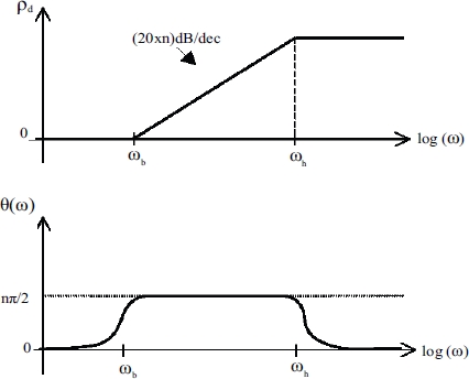
Figure 2.1. Theoretical Bode diagrams of 
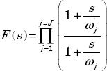
Let ![]() be the approximation of
be the approximation of ![]() in the frequency band
in the frequency band ![]() , using a product of J lead/lag cells:
, using a product of J lead/lag cells:

The success of this methodology is a consequence of its parsimony. Let us recall that the objective of this synthesis is to be efficient on a several-decade frequency band. An arithmetic distribution of frequencies ![]() would lead to an explosion of the number of cells. On the contrary, the choice of a geometric distribution, in adequation with the logarithmic scale log(ω), leads to a realistic number of cells. The reader has to refer to the papers and books of Oustaloup for a geometric and theoretical proof of this technique and particularly to [OUS 00].
would lead to an explosion of the number of cells. On the contrary, the choice of a geometric distribution, in adequation with the logarithmic scale log(ω), leads to a realistic number of cells. The reader has to refer to the papers and books of Oustaloup for a geometric and theoretical proof of this technique and particularly to [OUS 00].
Let us recall the essential results.
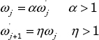
The filter ![]() composed of J cells is characterized by three synthesis parameters: α , η and n.
composed of J cells is characterized by three synthesis parameters: α , η and n.
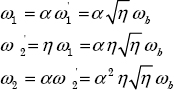
Let ![]() be the lower frequency close to ωb, and ωJ be the higher frequency close to ωh. The relations that
be the lower frequency close to ωb, and ωJ be the higher frequency close to ωh. The relations that ![]() and ωj frequencies have to verify are:
and ωj frequencies have to verify are:
If J, the total number of cells, is sufficiently high, the Bode diagram of ![]() in the band
in the band ![]() approximates
approximates ![]() , i.e. its modulus is characterized by a positive asymptote whose slope is equal to n×20 dB/dec and its constant phase is equal to
, i.e. its modulus is characterized by a positive asymptote whose slope is equal to n×20 dB/dec and its constant phase is equal to ![]() .
.
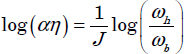
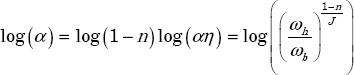
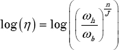
The parameters α and η are linked by the relation:
2.3. Frequency synthesis of the fractional integrator
2.3.1. Objective
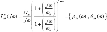
The objective of the frequency synthesis is to provide a realization of ![]() in the frequency domain. The corresponding modulus and phase are defined by:
in the frequency domain. The corresponding modulus and phase are defined by:
which lead to the Bode diagrams plotted in Figure 2.2.
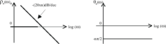
Figure 2.2. Theoretical Bode diagram of 
2.3.2. Direct method
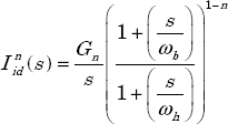
The permutation of frequencies ωb and ωh in equation [2.5] provides the approximation of ![]() in the frequency band
in the frequency band ![]() , thus:
, thus:

The corresponding Bode diagrams are represented in Figure 2.3.
Figure 2.3 represents the asymptotic diagram of this approximation and its comparison with the ideal diagram of ![]() .
.
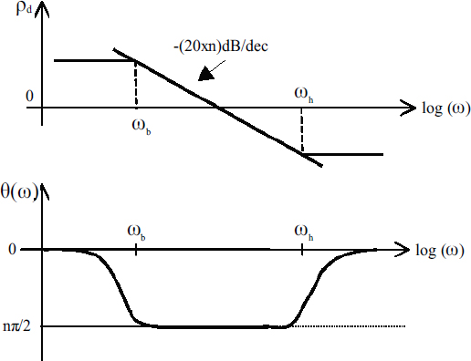
Figure 2.3. Asymptotic Bode diagrams of approximation
A direct consequence of this approximation is that ρ(ω) has a finite constant value for ω < ωb, whereas the ideal integrator is characterized by an infinite gain when ω → 0.
This concept of the static gain at ω → 0 presents no interest for the differentiator used in the Crone controller; on the contrary, it is essential for the integrator, because it is at the origin of a static error in the numerical simulation. This essential concept will be discussed in Chapter 6.
2.3.3. Indirect method
In order to impose an infinite gain at ω → 0 on the frequency approximation of ![]() , we use an indirect method for the integrator realization.
, we use an indirect method for the integrator realization.
The proposed solution is to include an integer order integrator for ω < ωb. The drawback of this technique is to distort the approximation slope for ω < ωb: it is equal to –20dB/dec for ω < ωb instead of –n×20dB/dec. On the contrary, its main interest is that the static gain tends to infinity for ω → 0, which is the necessary requirement to avoid static errors in the numerical simulation. It is important to note that the success of the indirect approximation is due to the inclusion of this integer order integrator (see Chapter 6).
Now, let us present the principle of this indirect method [TRI 99].
As ![]() introduces a constant slope equal to –20dB/dec and a constant phase equal to –π/2 on
introduces a constant slope equal to –20dB/dec and a constant phase equal to –π/2 on ![]() , it is necessary to modify the slope and the phase on
, it is necessary to modify the slope and the phase on ![]() , in order to obtain respectively –n×20dB/dec and –nπ/2.
, in order to obtain respectively –n×20dB/dec and –nπ/2.
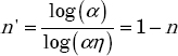
The solution is to incorporate a positive phase equal to +n'π/2 on this frequency band, in order to obtain a resulting phase equal to –nπ/2 on ![]() . Therefore, n' has to be chosen as:
. Therefore, n' has to be chosen as:
where n' is the order of the differentiator ![]() .
.
Let ![]() be the ideal approximation of
be the ideal approximation of ![]() on
on ![]() :
:
The asymptotic Bode diagrams of ![]() are presented in Figure 2.4.
are presented in Figure 2.4.

Figure 2.4. Asymptotic Bode diagrams of 
2.3.4. Frequency synthesis of 
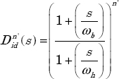
As a direct consequence of Oustaloup’s technique, the differentiator  is approximated by a product of lead/lag cells.
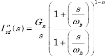
Therefore, the frequency approximation of ![]() , is defined by:
, is defined by:
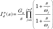
where Gn is a normalization coefficient.
The index “d” of ![]() is for discrete: the approximation is based on a product of J cells on
is for discrete: the approximation is based on a product of J cells on ![]() , i.e. the frequency band has been discretized into J values ωj, ranging from ωb to ωh.
, i.e. the frequency band has been discretized into J values ωj, ranging from ωb to ωh.
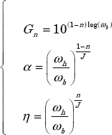
As mentioned previously, the differentiator ![]() is characterized by three parameters: α, η and 1−n.
is characterized by three parameters: α, η and 1−n.
Practically, the user defines ωb and ωh, the number of cells J + 1 and the fractional order n. Gn, α and η are defined as (see Appendix A.2 and [BEN 08a]):
2.4. State space representation of 
The frequency approximation [2.15] of ![]() is perfectly suited for a physical realization of the fractional integrator based on electrical circuits, for example RC circuits. However, in the context of numerical simulation, a realization based on a system of first-order ODEs, i.e. a state space representation, is necessary.
is perfectly suited for a physical realization of the fractional integrator based on electrical circuits, for example RC circuits. However, in the context of numerical simulation, a realization based on a system of first-order ODEs, i.e. a state space representation, is necessary.
Equation [2.15] defining ![]() , with input v(t) and output x(t) , can be represented by the graph of Figure 2.5.
, with input v(t) and output x(t) , can be represented by the graph of Figure 2.5.
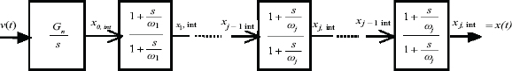
Figure 2.5. Block diagram representation of 
The state space model [LIN 01a] is characterized by the internal state variables ![]() (j = 0 to J) (“int” for integrator).
(j = 0 to J) (“int” for integrator).
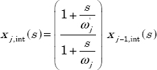
The jth order elementary cell is characterized by the input/output equation:
corresponding to the ODE:
As ![]() , we can write, for j = 0 to J:
, we can write, for j = 0 to J:
with
Note that, for ![]()
so ![]() .
.
All of these ODEs correspond to a global state space model [TRI 99], with input v(t) and output x(t) such that:
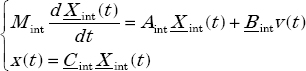
where
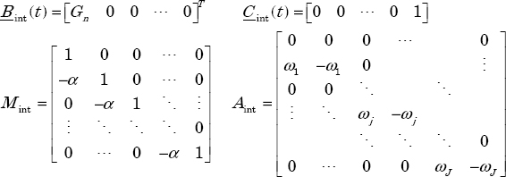
As the matrix Mint is invertible, we can transform this system into a conventional form:
Nevertheless, we lose the benefit of Mint and Aint matrix parsimony, because the resulting matrix ![]() is full.
is full.
Note that we can bypass this problem by a recursive integration of the differential system.
The numerical integration of:
provides x0,int (t) , based on input v(t) . Then, with knowledge of x0,int (t) , the numerical integration of the next differential equation:
provides x1,int (t) and so on.
Finally, this recursive procedure provides xJ,int (t) , i.e. x(t) .
However, even with this simple recursive procedure, the state space model remains relatively complex; moreover, it hides an essential specificity of ![]() .
.
2.5. Modal representation of 
The initial representation of ![]() , composed of a product of J +1 cells, can be converted into a sum of elementary cells, i.e.
, composed of a product of J +1 cells, can be converted into a sum of elementary cells, i.e. ![]() can be represented in a modal form, which is the fundamental link between frequency and time approaches (see Chapter 6).
can be represented in a modal form, which is the fundamental link between frequency and time approaches (see Chapter 6).
Of course, because all the terms ![]() are different, we can use the partial fraction expansion [POI 03, BEN 08a]:
are different, we can use the partial fraction expansion [POI 03, BEN 08a]:

In order to satisfy this equality, only the coefficient cj has to be calculated. Using the well-known partial fraction expansion technique, we can write for cj:

This modal model can be represented by the diagram of Figure 2.6.
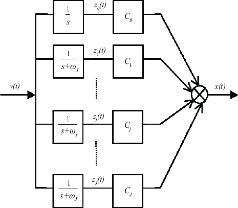
Figure 2.6. Modal representation of 
This model is characterized by the internal state variables zj(t) :
i.e.
This means that ![]() can be represented by the state space modal form:
can be represented by the state space modal form:
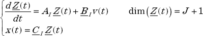
with
This modal system is obviously more simple to use than the previous one. A direct consequence is the simplification of the numerical simulation.
Another consequence is a different interpretation of the impulse response  .
.
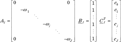
Let ![]() be the impulse response of the elementary cell
be the impulse response of the elementary cell ![]() .
.
Then:
with
Therefore
For v(t) = δ(t), we obtain x(t) = hn,d(t)
Therefore
This means that the impulse response hn,d(t) is the sum of J +1 modes ![]() ranging from
ranging from ![]() (including ω0 = 0).
(including ω0 = 0).
In other words, hn,d(t) is the weighted sum of very slow modes (explaining long memory behavior) and very fast modes. This fundamental concept will be formalized in Chapter 6.
Another point concerns the state variables of ![]() .
.
Let us recall that ![]() is the input/output representation of
is the input/output representation of ![]() .
.
According to [2.21] and [2.31], at least two state space models can be associated with ![]() , characterized respectively by the state variables Xint(t) and Z(t).
, characterized respectively by the state variables Xint(t) and Z(t).
It would be a nonsense to say that x(t) is the state variable characterizing the fractional integrator: obviously, the state variables are necessarily Xint(t) or Z(t), in fact an infinity of possibilities according to linear systems theory.
However, for a long time, x(t) has been considered as the state variable of the fractional integrator, as a result of a direct generalization of the integer order integrator to the fractional one.
As demonstrated previously, x(t) is only the output of ![]() , and is a pseudo-state variable, whereas Xint(t) or Z(t) are true internal state variables [TRI 09b, SAB 14].
, and is a pseudo-state variable, whereas Xint(t) or Z(t) are true internal state variables [TRI 09b, SAB 14].
REMARK 1.– In Chapter 6, the fractional integrator ![]() will be defined by a time approach using the inverse Laplace transform of
will be defined by a time approach using the inverse Laplace transform of ![]() . This integrator will be analyzed and compared to the frequency approach integrator. It can be concluded that the two approaches are equivalent. Therefore, in order to avoid confusion between different terminologies, the previous fractional integrator [2.31] will be called the infinite state integrator afterwards.
. This integrator will be analyzed and compared to the frequency approach integrator. It can be concluded that the two approaches are equivalent. Therefore, in order to avoid confusion between different terminologies, the previous fractional integrator [2.31] will be called the infinite state integrator afterwards.
2.6. Numerical algorithm
We have proposed a numerical simulation methodology with the first state model characterized by Xint (t) . In fact, the modal model is much more simple and better suited to the numerical simulation.
Practically, the modal model:
is discretized in the time domain (![]() , where Te is the sampling period) using the Z-transform [KRA 92], with a zeroth-order holder for input v(t) (i.e. v(t) is assumed to be constant between two steps).
, where Te is the sampling period) using the Z-transform [KRA 92], with a zeroth-order holder for input v(t) (i.e. v(t) is assumed to be constant between two steps).
Then:
where

and
Finally,
Note that j is the index for frequency discretization (modal discretization), whereas k is the index for time discretization.
Note that the modal model could have been simulated with Euler’s technique, i.e. equation [2.36] could have been transformed into a difference equation:
This difference equation would remain stable if:
In particular, for j = J , we have to respect ![]() , where ωJ is the higher frequency. Consequently, Euler’s technique (or Runge–Kutta’s technique) imposes a maximal value for Te, depending on ωJ. Note that there is no stability problem with the Z-transform technique.
, where ωJ is the higher frequency. Consequently, Euler’s technique (or Runge–Kutta’s technique) imposes a maximal value for Te, depending on ωJ. Note that there is no stability problem with the Z-transform technique.
2.7. Frequency validation
It is necessary to validate, in both frequency and time domains, theoretical results of the proposed frequency synthesis of the fractional order integrator. First, it is important to evaluate the influence of the number of cells on the frequency approximation of the theoretical reference model [2.14] (with s = jω):
A frequency interval (ωb =10−4 rad/s ; ωh = 10+4 rad/s ) and a fractional order (n = 0.5) have been imposed and the influence of J (J = 10;20;30;40) has been tested (note that the total number of cells is J+1, including the mode ω0 = 0).
Let us define the approximate fractional integrator:
with ρdB(ω) = 20log ρ(ω)
θ(ω) is expressed in degrees.
As it is not significant to compare directly ![]() and
and ![]() because the corresponding graphs are too close to each other, we show the errors:
because the corresponding graphs are too close to each other, we show the errors:
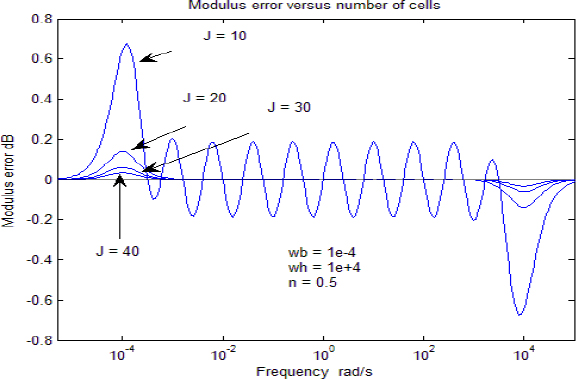
As expected, these errors are maximal for J=10 and followed by an important decrease for J=20 (and obviously for J=30 and J=40). Therefore, we can conclude that the geometrical distribution is very efficient and the result is acceptable, even with J=10 and an eight-decade frequency interval!

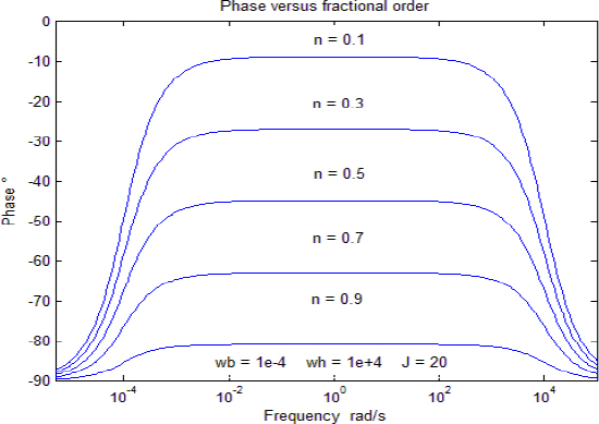
Finally, we show the graphs ρdB(ω) in Figure 2.9.

Figure 2.9. Modulus with different fractional orders
and θ°(ω) for increasing values of fractional order ![]() with the same frequency interval ωb =10−4 rad/s ; ωh=10+4 rad/s and J=20.
with the same frequency interval ωb =10−4 rad/s ; ωh=10+4 rad/s and J=20.
2.8. Time validation
Of course, the second necessary validation has to concern the ability of ![]() to perform the Riemann–Liouville integration.
to perform the Riemann–Liouville integration.
We have used a function v(t) composed of time-delayed step functions because it is straightforward to calculate the corresponding Riemann–Liouville integral.
Note that the step function v(t)=U H(t) corresponds to ![]() , thus
, thus
v(t) and xth(t) are defined as:
Note that v(t)=0 for T ≤ t < 2T, so we can observe the free response of the fractional integrator on this interval.
The response xIS(t) of ![]() has been computed with the numerical algorithm (see [2.37]–[2.40]) with the following parameters:
has been computed with the numerical algorithm (see [2.37]–[2.40]) with the following parameters:
The graphs of xth (t) and xIS (t) are shown in Figure 2.11.

Figure 2.11. Theoretical and simulated responses
As expected, these graphs fit perfectly.
In order to evaluate the accuracy of the infinite state simulation method, we present in Figure 2.12 the simulation error:
for two cases:
- 1)

- 2)


Figure 2.12. Simulation precision
We note that for case 2, the simulation error is divided by 10 compared to case 1. Nevertheless, even for case 1, the simulation error is acceptable.
We also present in Figure 2.13 the response x1(t) to v(t) of an integer order integrator in order to compare xIS(t) to x1(t) .
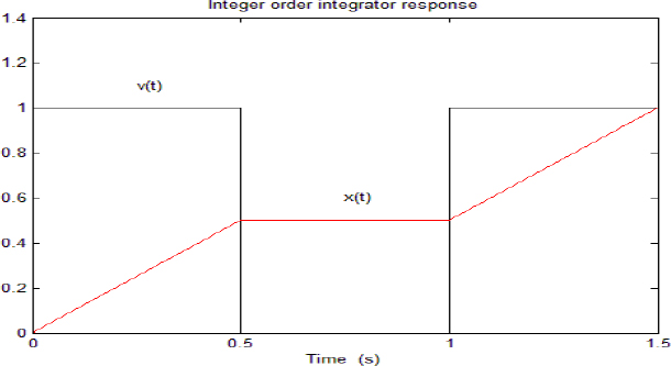
Figure 2.13. Response of the integer order integrator
Note that v(t)=0 for T ≤ t < 2T , so we can compare the two free responses on this interval.
For n = 1, we see that x1(t) = x1(T) = cte for T ≤ t < 2T, whereas for n=0.5, we see that xIS(t) is decreasing. This difference between the two free responses is a fundamental feature of the fractional integrator.
2.9. Internal state variables
As has already been highlighted, x(t) does not represent the state of the fractional integrator. It is only its output, resulting in the action of the different components of its internal state Z(t). Thus
Of course, it is interesting to visualize this distributed state. However, it is difficult to display each component zj (t). Therefore, we have preferred to use a global representation: Figure 2.14 shows the state vector Z (t) at four instants (0, T, 2T, 3T). At each instant, we represent the amplitude of zj (t) versus the index j of the frequency mode ωj with:
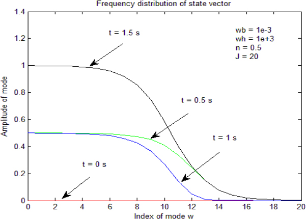
Figure 2.14. Approximate frequency distribution of z(ω,t)
The resulting graph is an approximation of the continuous frequency distribution z(ω,t), where ω ranges from 0 to ∞.
Note that the mode j=0 corresponds to ω0=0, i.e. to the integer order integrator included in the frequency approximation (see [2.33]). Therefore, we can verify that this integer order integrator behaves exactly as in Figure 2.13. In particular, note that its amplitude remains constant when v(t) = 0 on T ≤ t < 2T. The low frequency components also behave approximately as the component at j = 0. On the contrary, the high frequency modes quickly decrease on this interval, i.e. they explain the decrease in free response xIS (t).
A.2. Appendix: design of fractional integrator parameters
The objective is to define the design parameters Gn, α and η [BEN 08a].
A.2.1. Definition of Gn
First, we consider the ideal derivator ![]() with n’ = 1–n:
with n’ = 1–n:
Consider its asymptotic Bode diagram ![]() presented in Figure 2.15.
presented in Figure 2.15.
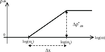
Figure 2.15. Asymptotic Bode diagram 
Let
and
Let

i.e. H(s) corresponds to ![]() without normalizing coefficient Gn and consider its asymptotic Bode diagram
without normalizing coefficient Gn and consider its asymptotic Bode diagram ![]() .
.
Then
and
Thus
Finally, consider the normalized filter:
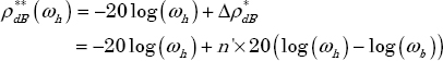
Its modulus ρdB verifies the relation:
Thanks to Gn, we want that the asymptotic Bode diagram of ![]() corresponds to
corresponds to ![]() at frequencies ωb and ωh:
at frequencies ωb and ωh:
Therefore, at ω=ωb:
Thus
Therefore, we obtain:
Of course, we verify that:
A.2.2. Definition of α and η
We are interested by
with

Different choices are possible for α and η, depending on the relation between ωb and ![]() , ωh and ωJ.
, ωh and ωJ.
We have used the choice:

or
Let us recall that:
Therefore, for J cells:
Thus
i.e.

or:
As
we obtain
i.e.

Then
i.e.
or
