
6
The Distributed Model of the Fractional Integrator
6.1. Introduction
In Part 1, and more specifically in Chapters 1 and 2, the Riemann–Liouville integration was defined, with a particular focus on the fractional order integrator. This operator was synthesized according to a frequency approach. Moreover, thanks to a partial fraction expansion, a modal representation was introduced. This result was not straightforward, considering the classical form of the integrator impulse response:
However, an important question is related to the limit of this modal model when the number of terms is increased to infinity.
The answer to this question is provided by the frequency distributed model of the fractional integrator, as a result of the inverse Laplace transform of ![]() . This model provides answers to fundamental questions, for example, on the relation between frequency and modal representations, the expression of the Riemann–Liouville integral at any initial instant t0 and more globally on the internal distributed state z(ω, t) of the integrator.
. This model provides answers to fundamental questions, for example, on the relation between frequency and modal representations, the expression of the Riemann–Liouville integral at any initial instant t0 and more globally on the internal distributed state z(ω, t) of the integrator.
Fundamentally, it will be demonstrated that the Riemann–Liouville integral of any function v(t) is a convolution between the impulse response hn (t) and v(t) , i.e. this integral can be interpreted as the response of an infinite dimension system. This convolution interpretation demonstrates that initialization of the fractional integrator obeys the same laws as any linear system [TRI 12a].
The last part of this chapter is dedicated to a physical interpretation of the distributed model thanks to the comparison of the fractional integrator with an infinite length RC diffusive line [MAA 14].
6.2. Origin of the frequency distributed model
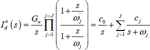
The fractional integrator In(s) is defined as the Laplace transform of its impulse response hn(t):
with ![]() .
.
Reciprocally, the inverse Laplace transform [SPI 65, LEP 80] of ![]() provides hn(t). However, hn(t) is not obtained directly: we obtain an intermediary model, which is the frequency distributed model.
provides hn(t). However, hn(t) is not obtained directly: we obtain an intermediary model, which is the frequency distributed model.
Let:
with

This integral is calculated with a Bromwich contour [LEP 80]. As the function In (s) is multiform with a branch point in s = 0, we use a cut in the complex plane, which leads to a modified Bromwich contour (for more details, see Appendix A6).
Therefore, we obtain:

Let us define a weighting function:
Then:
Note that this equation is similar to the discrete one obtained in Chapter 2:
Equation [6.7] is the limit of [6.8] when the interval between two consecutive modes ωj and ωj+1 tends to 0.
Equation [6.7] provides a new interpretation of hn(t), but does it correspond to definition [6.1]?
Let us define u = ω t, then:
Let us recall (Chapter 1, Appendix A.1.4):
we obtain finally:
Therefore, we verify whether the two expressions of hn(t) are equivalent, which can be summarized by:
An essential interest of [6.7] is to highlight that hn(t) is the result of an infinite dimension sum of e−ωt modes, weighted by µn(ω), where ω varies from 0 to ∞.
Equation [6.1] shows that hn(t) is characterized by long memory (when t ⟶ ∞), due to tn−1, equivalently to the action of very low frequency modes (ω ⟶ 0). On the contrary, for very short times (t ⟶ 0), it is the action of high frequency modes (ω ⟶ ∞) that is predominant, leading to ![]() .
.
Let us apply the Laplace transform to equation [6.7], then:

As
we obtain a fundamental result:
6.3. Frequency distributed model
Let us recall that the integrator In(s) is defined by the convolution equation:
or equivalently
where hn(t) is defined as:
Note that e–ωt is the impulse response of the elementary transfer function ![]() , corresponding to the impulsive input v(t) = δ(t). On the contrary, equation [6.19] means that x(t) = hn(t) is the weighted integral of all of these elementary impulse responses e–ωt.
, corresponding to the impulsive input v(t) = δ(t). On the contrary, equation [6.19] means that x(t) = hn(t) is the weighted integral of all of these elementary impulse responses e–ωt.
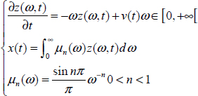
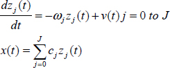
Let z(ω,t) be the elementary response of the transfer function ![]() to any input v(t). Therefore, z(ω,t) is the solution of the differential equation:
to any input v(t). Therefore, z(ω,t) is the solution of the differential equation:
Note that ![]() is replaced by
is replaced by ![]() since z(ω,t) is a function of two variables, ω and t.
since z(ω,t) is a function of two variables, ω and t.
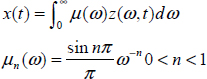
Thus, the convolution equation x(t) = hn(t)*v(t) can be interpreted as a frequency distributed differential system:
REMARK 1.– The integer order integrator corresponds to n = 1. This integer order operator is characterized by only one mode ω = 0.
SO ![]()
Moreover, the weighting function µn(ω) becomes a Dirac impulse µ1 (ω) = δ(ω) and:
REMARK 2.– The frequency distributed model of the fractional integrator is also called the diffusive representation model [MON 98]. The “diffusive” term can create a confusion with the diffusive equation. We will show in the last part of this chapter that there is some equivalence between the distributed model and the diffusive equation, but it is another problem.
We prefer to qualify [6.21] as the frequency distributed model of ![]() , where the variables z(ω,t) are distributed state variables.
, where the variables z(ω,t) are distributed state variables.
Moreover, because this infinite dimension distributed model is the basis of a methodology for the modeling of FDSs, we characterize this methodology as the infinite state approach.
6.4. Finite dimension approximation of the fractional integrator
Equations [6.21] represent the theoretical distributed model of ![]() . However, this model is not adapted to the numerical simulation of the operator.
. However, this model is not adapted to the numerical simulation of the operator.
This numerical simulation requires the discretization of the weighting function µn(ω). The simplest numerical approximation is based on a stepwise discretization, according to Figure 6.1, i.e. the distributed differential equation [6.21] is replaced, for frequency ωj, by:
Moreover, the integral:
becomes:
Let us define:
which is the area of the step j.
Therefore:
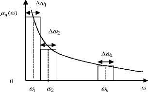
Figure 6.1. Discretization of the weighting function
6.5. Frequency synthesis and distributed model
Let us recall remember that thanks to the partial fraction expansion used in Chapter 2, section 2.5, it is possible to define a modal model:
Equations [6.25] and [6.26] are equivalent, except for the first frequency (ω0 = 0).
Moreover, it is important to note that frequencies ωj should not be chosen according to an arithmetic law, due to the very slow decrease of ω–n.
Any frequency discretization can be used; however, the previous geometric distribution defined in Chapter 2 is a powerful guide.
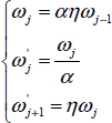
Therefore, using this geometric distribution for equation [6.24], frequencies ωj verify:
with

Nevertheless, it is important to remind that [6.25] starts at j = 1, whereas [6.26] starts at j = 0, with ω0 = 0.
Because lim ![]() , it is not possible to include ω0 = 0 in equation [6.25].
, it is not possible to include ω0 = 0 in equation [6.25].
Nevertheless, this inclusion is necessary, as demonstrated thereafter.
Consider the unit step response of the system ![]() , so
, so
Recall that ![]() .
.
Thus, if we use approximation [6.25]:
we obtain

which means that there is a static error, regardless of the discretization procedure.
On the contrary, if we use approximation [6.26]:

Thus, it is equation [6.26] starting at j = 0, with ω0 = 0 , that provides the best approximation of the fractional integrator (see Chapter 2).
Therefore, we can conclude that the frequency distributed model [6.21] provides the theoretical justification of equation [6.26], without modification of the conclusions presented in Chapter 2.
Moreover, we can use equation [6.16] to understand the connection between the frequency response and the modal representation of the fractional integrator.
Let us recall that the frequency response of In (s) is defined as:
where u varies from 0 to +∞.
The modal representation is defined by the distribution µn(ω) of modes ω, verifying equation [6.16]:
where ω varies from 0 to +∞.
Thus, the frequency response of the modal model is defined by:

where ω and u vary from 0 to +∞.
Note that it is essential to avoid confusion between variables u (for the frequency response) and ω (for the modal distribution).
6.6. Numerical validation of the distributed model
In order to verify the equivalence between the frequency model and the distributed model, we propose the following two numerical computations.
6.6.1. Reconstruction of the weighting function
Consider the frequency model defined in Chapter 2.
The equivalence between equations [6.25] and [6.26] implies:
i.e. αj ≡ cj
where αj = µn(ωj)Δωj.
Therefore, the µn(ωj) weighting function can be reconstructed using
with
![]() (see Chapter 2).
(see Chapter 2).
For this numerical computation, we use the following values:
We present in Figure 6.2 the theoretical curve ![]() and the numerical values obtained with equation [6.39], using log/log coordinates.
and the numerical values obtained with equation [6.39], using log/log coordinates.
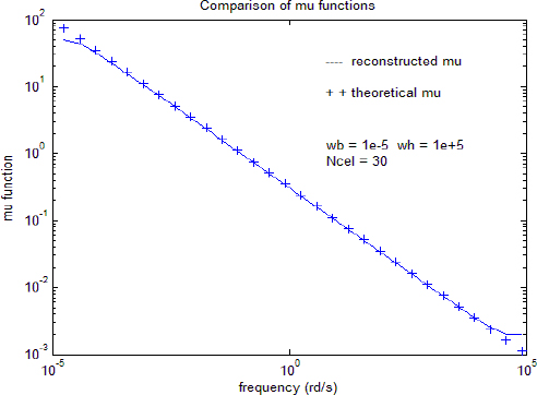
Figure 6.2. Comparison of weighting functions
Inside the frequency interval ![]() , we can note a perfect equivalence between the theoretical and computed values.
, we can note a perfect equivalence between the theoretical and computed values.
Differences appear at:
- – high frequencies, for ω>103 rad/s: frequency synthesis is not valid for ω>ωh, so there is a necessary difference for ω>103 rad/s ;
- – low frequencies, for ω>10−3 rad/s: because we have introduced an integer integrator, in order to obtain an infinite static gain for ω ⟶ 0, there is a necessary difference for ω < ωb.
6.6.2. Reconstruction of the impulse response
The frequency distributed model corresponds to:
If v(t) = δ(t), the response x(t) corresponds to the impulse response ![]() of the frequency discretized model.
of the frequency discretized model.
As v(t) = δ(t), we obtain ![]()
whereas [6.1] shows that ![]() .
.
The main difference between ![]() and hn(t) corresponds to t = 0:
and hn(t) corresponds to t = 0:
hn (0) ⟶∞, whereas ![]() is a finite value.
is a finite value.
In Figure 6.3, we compare ![]() and hn(t) with the previous values [6.41].
and hn(t) with the previous values [6.41].
The two impulse responses are compared on the interval [0;100s] with Te=10–3 s.
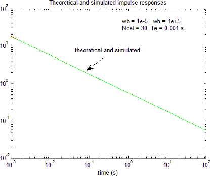
Figure 6.3. Comparison of impulse responses
We note a perfect equivalence in the interval [0; 100s].
We can conclude that either the reconstruction of the weighting function or the reconstruction of the impulse response confirms that the distributed frequency model defined in Chapter 2 converges asymptotically to the ideal model provided by the inverse Laplace transform of ![]() .
.
6.7. Riemann–Liouville integration and convolution
In Chapter 1, we introduced a simplified definition of the Riemann–Liouville integral:

where the lower bound of the integral is equal to 0. Remember that this simplified formulation of the Riemann–Liouville integral can be used to define the fractional integrator.
Now, we use a more general definition of this integral.
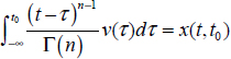
Let ![]() be the Riemann–Liouville integral where the lower bound is equal to a, with a∈R, i.e.:
be the Riemann–Liouville integral where the lower bound is equal to a, with a∈R, i.e.:

This expression, where ![]() represents the convolution between hn(t) and v(t), is not adapted to a general system theory formulation.
represents the convolution between hn(t) and v(t), is not adapted to a general system theory formulation.
Obviously, we can refer to the previous distributed definition [6.19]:
Let v(t) be an input defined for ![]() and consider
and consider ![]() , i.e. with a lower bound equal to —∞. Thus, we take into account all the past of v(t).
, i.e. with a lower bound equal to —∞. Thus, we take into account all the past of v(t).
Let us recall the distributed differential equation:
where z(ω,t) is the result of a convolution [ZEM 65, KRA 92, SCH 98] between e−ωt and v(t) (where e–ωt is the impulse response of the elementary system ![]() ).
).
Therefore
and
Consider an instant ![]() .
.
We propose to express x(t) using ![]() . We can write [6.47] as:
. We can write [6.47] as:
where
As:
We obtain:
where z(ω,t0) is the elementary distributed state of the fractional integrator at instant t0 : z(ω,t0) summarizes the past of the integrator for the elementary frequency ω, i.e. the contribution of v(t) at frequency ω for t < t0 (since t = –∞).
Therefore, in equation [6.51], the first term represents the free response of the integrator for t ≥ t0, based on the distributed initial condition z(ω,t0), whereas the second term corresponds to the forced response of the integrator for t≥t0. We recognize the general expression of a linear system response [ZAD 08, WIB 71, KAI 80], the sum of a free response and a forced response, where the initial condition (here z(ω,t0), with ω varying from 0 to ∞) summarizes the past (or pre-history) of the system at t = t0.
Obviously, any instant t0 can verify [6.51]: so we can choose t0 = 0, which makes it possible to use the Laplace transform.
Let z (ω,0) be the initial condition at t0 = 0.
Then, the Laplace transform applied to the distributed differential equation yields:
so
and
As (equation [6.16]):
we obtain finally:
corresponding in the time domain to:
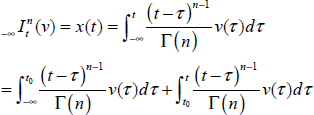
REMARK 3.– Let us recall that the integer order integration is a particular case of the fractional order integration with n = 1 (µn(ω) is replaced by δ(ω) for n = 1):
Therefore
as H(t–τ) = 1 for τ ≤ t.
The convolution integral is in fact a simple integration in the integer order case.
Thus, with an instant ![]() , we can write:
, we can write:
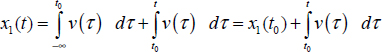
where x1 (t0) is the initial condition of the integrator at t = t0.
Therefore:
If we use ![]() , we can write
, we can write
As a generalization of the integer order case, it would be tempting to write:
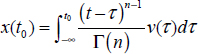
where x(t0) would be the initial condition of the Riemann–Liouville integral at t0.
In fact:
where x(t,t0) depends on t and t0.
Obviously, it is wrong to use equations [6.62] and [6.63] because x(t,t0) is not a constant.
Note that:
Therefore:
In other words, equation [6.61] is correct only at t = t0, but it is not able to predict x(t) for t > t0.
This misuse of the convolution integral [6.61] is unfortunately at the origin of many errors in the definition of the initial conditions of fractional derivatives.
6.7.1. Conclusion
We have established a fundamental result: fractional integration is a convolution process which can be expressed using the linear system theory, thanks to the distributed model of the fractional integrator.
Note that the Riemann–Liouville integral of f(t) can be formulated as ![]() using any instant t0 (t0 = 0 in practice), if we take into account the past (t < t0) using the distributed initial condition z(ω,t0).
using any instant t0 (t0 = 0 in practice), if we take into account the past (t < t0) using the distributed initial condition z(ω,t0).
Moreover, this fundamental result has many consequences: it is used to characterize the transients of FDEs or FDSs (Chapter 7) and those of the Riemann–Liouville and Caputo fractional derivatives (Chapter 8).
6.8. Physical interpretation of the frequency distributed model
6.8.1. The infinite RC transmission line
Electrical lines were used during the 19th Century across the Atlantic Ocean to transmit telegraph messages. Theory of these transmission lines was established by Thomson and particularly by Heaviside who formulated the telegrapher’s equations, which were an adaptation of Maxwell’s equations [BEN 79]. When the inductor effect is negligible, the transmission line is equivalent to an RC line. Heaviside demonstrated that the RC line behaves as a fractional integrator [OLD 74, MIL 93]. Based on this equivalence, we propose to provide a physical interpretation of the distributed infinite state model and its distributed state variable z(ω,t).
Consider the RC line elementary cell shown in Figure 6.4 [OLD 74, FAR 82].
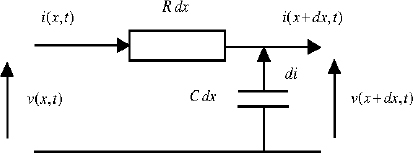
Figure 6.4. RC line elementary cell
are capacity and resistance densities.
This elementary cell is governed by the voltage/current equations:
corresponding to the well-known partial derivative diffusion equation [KOR 68, FAR 82]:
Consider an infinite length transmission line. The general solution of [6.68] is easily obtained using the Laplace transform, as in Chapter 4.
Let us define:
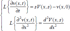
Assuming that v(x, 0) = 0 ∀x, [6.68] is equivalent to the differential equation:
whose general solution is:
where B depends on the excitation at the terminal x = 0 of the transmission line.
Using [6.68], we obtain:
Let us define the impedance of the RC line as
Then:
This result means that the infinite RC line behaves like a fractional integrator, with a fractional order equal to 0.5.
6.8.2. RC line and spatial Fourier transform
The infinite dimension RC line is characterized by the variables v(x,t),i(x,t) with the condition:
The RC line variables at terminal x = 0 are v(0, t) and i(0, t).
Let us define
which is the spatial Fourier transform [KRA 92] of v(x, t).
The Fourier transform of  is defined as:
with the condition:
Thus, the Fourier transform of is equal to:
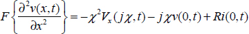
Therefore, the Fourier transform of equation [6.67] is:
Thanks to [6.79], this equation is equivalent to two differential systems:
The solutions ![]() and
and ![]() are characterized by:
are characterized by:
Reciprocally, if ![]() is known, we obtain v(x,t) using the inverse Fourier transform:
is known, we obtain v(x,t) using the inverse Fourier transform:
6.8.3. Impulse response of the RC line
We are interested in v(0,t) when i(0,t) = δ(t). According to [6.88]:
Therefore
According to [6.87]
where ![]() is the solution of the differential equation [6.85], with
is the solution of the differential equation [6.85], with ![]() .
.
is the solution of [6.85] for ![]() and also for
and also for ![]() .
.
Hence:
and:
We finally obtain:
Let us recall that the impulse response of a fractional integrator is ![]() .
.
Therefore, for n = 0.5:
Thus:
Obviously, this result expressed in the time domain is equivalent to [6.75] expressed in the s variable Laplace transform domain.
On the contrary, because v(0,t) is obtained using [6.85] and [6.91], we can compare the following two differential systems:
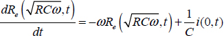
- – for the fractional integrator, the output y(t) is the solution of the distributed system:
- – for the transmission line, the output v(0,t) is the solution of the distributed system:
Equations [6.99], [6.100] and [6.101], [6.102] are analogous, so:
Note that ![]() .
.
Therefore:

Consequently, the two expressions have the same physical dimension. The main conclusion is that according to [6.103], the distributed model of the fractional integrator, where the time frequency ω ranges from 0 to ∞, corresponds to the Fourier transform model of the RC line, where the spatial frequency ![]() ranges from –∞ to +∞.
ranges from –∞ to +∞.
6.8.4. General solution
The previous result can be generalized to any excitation i(0, t) according to the equivalence:
Equation [6.101] can be expressed as:
and according to [6.93]:
Therefore:
Note that:
hence:

On the contrary, using system [6.99] with v(t) = i(0,t) and comparing the two differential systems, we obtain:
Hence, using z(ω,t) in [6.102], we obtain:
[6.112] can be expressed as:
which corresponds to the distributed model of the fractional integrator with:
Conclusion
The fractional integrator, with order equal to 0.5, is exactly equivalent to an infinite dimension RC line, i.e. to an infinite dimensional partial differential diffusive equation. The frequency distributed model of the integrator corresponds to the real part of the spatial Fourier transform of the diffusive system. The modes ω of the integrator distributed model correspond to the spatial frequencies ![]() of the harmonic diffusive response.
of the harmonic diffusive response.
6.8.5. Initialization in the time and spatial domains
It is well known [KOR 68, FAR 82] that the initial condition of the diffusive RC line corresponds to v(x, 0), x ranging from 0 to ∞. On the contrary, the initial condition of the fractional integrator distributed model is z(ω,0), ω ranging from 0 to ∞.
According to the equivalence:
and the definition:
the frequency distributed initial condition z(ω, 0) is directly equivalent to the spatial distributed initial condition v(x, 0):
Initialization of the RC line with v(x, 0) requires knowledge of the initial voltage, particularly for large values of x. Recall that due to the Fourier transform, large values of x correspond to low frequency values of ![]() . Therefore, initialization of the integrator with z(ω, 0) requires knowledge of ω for any value of the frequency spectrum, particularly for very low values of ω, exhibiting the specificity of the long range memory of a fractional system.
. Therefore, initialization of the integrator with z(ω, 0) requires knowledge of ω for any value of the frequency spectrum, particularly for very low values of ω, exhibiting the specificity of the long range memory of a fractional system.
This equivalence between the fractional integrator and the RC line will be used in Chapter 5 Volume 2 to derive a technique for the control of the distributed state v(x,t) of the RC line.
A.6. Appendix: inverse Laplace transform of the fractional integrator
Let ![]() .
.
Reciprocally, for a given transfer function H(s), h(t) is provided by the inverse Laplace transform ![]()

The integral is calculated using a Bromwich contour [LEP 80].

Figure 6.5. Modified Bromwich contour C
As ![]() is a multiform function, a cut is necessary in the complex plane, which leads to the modified Bromwich contour presented in Figure 6.5:
is a multiform function, a cut is necessary in the complex plane, which leads to the modified Bromwich contour presented in Figure 6.5:
Thus, we can write:
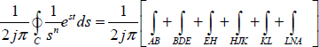
Referring to Cauchy’s theorem [KOR 68, LEP 80]:
As
then:

Finally, we obtain
Physical considerations indicate that x corresponds to a frequency ω, so let us define ω = x.
Note that e–ω t is the impulse response (z(ω, t) = e-ωt) of the elementary system ![]() when its input is v(t) = δ(t).
when its input is v(t) = δ(t).
Finally, equation [6.124] means that hn(t) is the weighted contribution of all these elementary systems, with ω ranging from ω = 0 to ∞, where the frequency weight is
Therefore