SQL Server executes a query by a set of physical operators. Because these operators iterate through rowsets, they are also called iterators. There are different join operators, because when performing joins, SQL Server uses different algorithms. SQL Server supports three basic algorithms: nested loops joins, merge joins, and hash joins.
The nested loops algorithm is a very simple and, in many cases, efficient algorithm. SQL Server uses one table for the outer loop, typically the table with the fewest rows. For each row in this outer input, SQL Server seeks matching rows in the second table, which is the inner table. SQL Server uses the join condition to find the matching rows. The join can be a non-equijoin, meaning that the equality operator does not need to be part of the join predicate. If the inner table has no supporting index to perform seeks, then SQL Server scans the inner input for each row of the outer input. This is not an efficient scenario. A nested loop join is efficient when SQL Server can perform an index seek in the inner input.
Merge join is a very efficient join algorithm. However, it has its own limitations. It needs at least one equijoin predicate and sorted inputs from both sides. This means that the merge join should be supported by indexes on both tables involved in the join. In addition, if one input is much smaller than another, then the nested loop join could be more efficient than a merge join.
In a one-to-one or one-to-many scenario, a merge join scans both inputs only once. It starts by finding the first rows on both sides. If the end of the input is not reached, the merge join checks the join predicate to determine whether the rows match. If the rows match, they are added to the output. Then the algorithm checks the next rows from the other side and adds them to the output until they match the predicate. If the rows from the inputs do not match, then the algorithm reads the next row from the side with the lower value from the other side. It reads from this side and compares the row to the row from the other side until the value is bigger than the value from the other side. Then it continues reading from the other side, and so on. In a many-to-many scenario, the merge join algorithm uses a worktable to put the rows from one input side aside for reuse when duplicate matching rows are received from the other input.
If none of the input is supported by an index and an equijoin predicate is used, then the hash join algorithm might be the most efficient one. It uses a searching structure named a hash table. This is not a searching structure you can build, like a balanced tree used for indexes. SQL Server builds the hash table internally. It uses a hash function to split the rows from the smaller input into buckets. This is the build phase. SQL Server uses the smaller input for building the hash table because SQL Server wants to keep the hash table in memory. If it needs to get spilled out to tempdb on disk, then the algorithm might become much slower. The hash function creates buckets of approximately equal size.
After the hash table is built, SQL Server applies the hash function on each of the rows from the other input. It checks to see which bucket the row fits. Then it scans through all rows from the bucket. This phase is called the probe phase.
A hash join is a kind of compromise between creating a fully balanced tree index and then using a different join algorithm and performing a full scan of one side of the input for each row of the other input. At least in the first phase, a seek of the appropriate bucket is used. You might think that the hash join algorithm is not efficient. It is true that in single-thread mode, it is usually slower than the merge and nested loop join algorithms, which are supported by existing indexes.
However, SQL Server can split rows from the probe input in advance. It can push the filtering of rows that are candidates for a match with a specific hash bucket down to the storage engine. This kind of optimization of a hash join is called a bitmap filtered hash join. It is typically used in a data warehousing scenario, in which you can have large inputs for a query that might not be supported by indexes. In addition, SQL Server can parallelize query execution and perform partial joins in multiple threads. In data warehousing scenarios, it is not uncommon to have only a few concurrent users, so SQL Server can execute a query in parallel. Although a regular hash join can be executed in parallel as well, a bitmap filtered hash join is even more efficient because SQL Server can use bitmaps for early elimination of rows not used in the join from the bigger table involved in the join.
In the bitmap filtered hash join, SQL Server first creates a bitmap representation of a set of values from a dimension table to prefilter rows to join from a fact table. A bitmap filter is a bit array of m bits. Initially, all bits are set to 0. Then SQL Server defines k different hash functions. Each one maps some set elements to one of the m positions with a uniform random distribution. The number of hash functions k must be smaller than the number of bits in array m. SQL Server feeds each of the k hash functions to get k array positions with values from dimension keys. It set the bits at all these positions to 1. Then SQL Server tests the foreign keys from the fact table. To test whether any element is in the set, SQL Server feeds it to each of the k hash functions to get k array positions. If any of the bits at these positions are 0, the element is not in the set. If all are 1, then either the element is in the set, or the bits have been set to 1 during the insertion of other elements. The following figure shows the bitmap filtering process:
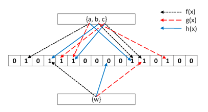
In the preceding figure, the length m of the bit array is 16. The number k of hash functions is 3. When feeding the hash functions with the values from the set {a, b, c}, which represents dimension keys, SQL Server sets bits at positions 2, 4, 5, 6, 11, 12, and 14 to 1 (starting numbering positions at 1). Then SQL Server feeds the same hash functions with the value w from the smaller set at the bottom {w}, which represents a key from a fact table. The functions set bits at positions 4, 9, and 12 to 1. However, the bit at position 9 is set to 0. Therefore, the value w is not in the set {a, b, c}.
Bitmap filters return so-called false positives. They never return false negatives. This means that when you declare that a probe value might be in the set, you still need to scan the set and compare it to each value from the set. The more false positive values a bitmap filter returns, the less efficient it is. Note that if the values in the probe side in the fact table are sorted, it will be quite easy to avoid the majority of false positives.
The following query reads the data from the tables introduced earlier in this section and implements star schema-optimized bitmap filtered hash joins:
USE WideWorldImportersDW;
SELECT cu.[Customer Key] AS CustomerKey, cu.Customer,
  ci.[City Key] AS CityKey, ci.City,
  ci.[State Province] AS StateProvince, ci.[Sales Territory] AS SalesTeritory,
  d.Date, d.[Calendar Month Label] AS CalendarMonth,
  d.[Calendar Year] AS CalendarYear,
  s.[Stock Item Key] AS StockItemKey, s.[Stock Item] AS Product, s.Color,
  e.[Employee Key] AS EmployeeKey, e.Employee,
  f.Quantity, f.[Total Excluding Tax] AS TotalAmount, f.Profit
FROM Fact.Sale AS f
  INNER JOIN Dimension.Customer AS cu
    ON f.[Customer Key] = cu.[Customer Key]
  INNER JOIN Dimension.City AS ci
    ON f.[City Key] = ci.[City Key]
  INNER JOIN Dimension.[Stock Item] AS s
    ON f.[Stock Item Key] = s.[Stock Item Key]
  INNER JOIN Dimension.Employee AS e
    ON f.[Salesperson Key] = e.[Employee Key]
  INNER JOIN Dimension.Date AS d
    ON f.[Delivery Date Key] = d.Date;
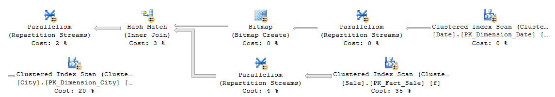
The following figure shows a part of the execution plan. Please note that you can get a different execution plan based on differences in resources available to SQL Server to execute this query. You can see the Bitmap Create operator, which is fed with values from the dimension date table. The filtering of the fact table is done in the Hash Match operator: