There are some points to go through before crafting a visualization. If your figure is meant to be part of an exploratory analysis for yourself only, you might not work so hard into details such as the font's family and size; the ugly default settings given by base R graphing are enough. On the other hand, if you wish to publish your figure, you may want to pay a great deal of attention to details.

Another question to ask is, what kind of data do you have at hand? How many variables do you wish to represent? Are they discrete or continuous? Is there an underlying logical ordering for them? If we are talking time series, data could make more sense if presented chronologically. Many things need to be thought about while you design plots. You are very likely to develop preferences of your own while you become experienced.

The two visualizations that I like the most when displaying the Twitter ranks are called lollipop plots and word clouds. Both can be done using R. We are about to breed both. The lollipops are a neat and clean way to show the difference between the most tweeted words; ggplot2 can be used to convey such a visualization. Install it using install.packages():

if(!require(ggplot2)){install.packages('ggplot2')}

We can use factors to rule an order to the lollipops we are about to draw:

clean_dt$word <- factor(clean_dt$word,
                        levels = rev(clean_dt$word))

Using ggplot2, it's possible to layer-wise conjure a lollipop plot:

library(ggplot2)

ggplot(data = clean_dt[1:10,], aes(x = n, y = word)) +
  geom_segment(linetype = 'dashed',
               size = .1,
               aes(yend = word, 
                   x = min(n) - 50, 
                   xend = n)) +
  geom_point(size = 17, color = '#e66101') +
  geom_text(aes(label = n), size = 6) +
  coord_cartesian(xlim = c(120, 500))

As a result, the following figure is generated:

The previous code may not be as friendly as you would expect, but read it layer by layer, and I am sure you will understand what is happening with a little aid from ggplot2's documentation. Aside from one being a visualization, both Figure 4.6 and object clean_dt displays an analysis called term frequency analysis.

There is another visualization that is very useful to display this kind of data: word clouds. Word clouds are the main concern from the wordcloud package. Perform a simple check or install drill with the following code:

if(!require(wordcloud)){install.packages('wordcloud')}
if(!require(tm)){install.packages('tm')}

Although the methods to craft the word cloud visualization come from the wordcloud package itself, missing the  tm package sometimes causes trouble. The previous code also seeks and installs the latter. Once we have done that, we can proceed to conjure a word cloud. Setting a seed number generator with set.seed() is not necessary, but it will make your results reproducible.

The function par() is used to set general graphical parameters for methods related to the base plot(). Next, the comment shows how it can be used to set smaller margins. Uncomment and run the following code in your word cloud to spread over the margins: 

#par(mar = rep(0,4))
library(wordcloud)
set.seed(10)
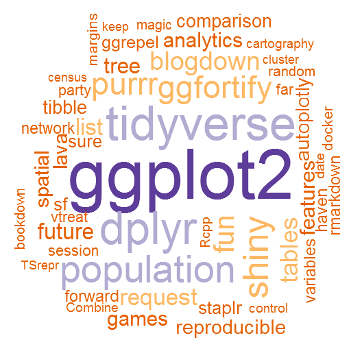
wordcloud(word = clean_dt$word, freq = clean_dt$n, random.order = F, 
          rot.per = .35, scale = c(5,.5), max.words = 50, 
          colors = c('#e66101','#fdb863','#b2abd2','#5e3c99'))

This is how the wordcloud package can be used to craft a word cloud. The result is displayed in the following figure. Before getting to it, let's navigate through the arguments that are used as input the wordcloud() function:

• word: A vector of words to be printed into the word cloud
• freq: The number of times each word appeared
• random.order: If you want the words that most appear to be printed first, set this argument to FALSE (or simply F)
• rot.per: Pick the probability of a word to be printed vertically; the way I did, about 35% of the words were printed vertically
• scale: A two-element vector ruling the size range of the words
• max.words: The maximum number of words to be printed
• colors: A color palette used to fill the words

It's much more fun to look at the results in the preceding figure than to look at a list of the most frequent 50 words; don't you agree? Following is the word cloud for R packages:

Notice how we still got many names that could be mistaken as R packages, as they refer to common words. We could color the words differently based on the packages we have already installed on our machines. Try the following code for this:

clean_dt$col <- '#b2abd2'
clean_dt$col[clean_dt$word %in% installed.packages()] <- '#e66101'
wordcloud(word = clean_dt$word[1:50], freq = clean_dt$n[1:50], 
          random.order = F, rot.per = .35, scale = c(5,.5),
          colors = clean_dt$col[1:50], ordered.colors = T)

With this amazing visualization, we close this section and move on the analysis.