With all the things in place, it's time to look at practical examples. Under this topic, we will build and store a deep learning model from scratch using Keras. To get started, we need a dataset. You might be thinking here comes MNIST data again. but not this time. We will look for data in the University of California, Irvine (UCI) Machine Learning Repository.

You can check all the UCI's datasets in the following link: https://archive.ics.uci.edu/ml/datasets.html

The dataset used is about credit card default. It can be found here: https://archive.ics.uci.edu/ml/datasets/default+of+credit+card+clients.

This data has 30,000 observations about credit card owners. The available variables go from credit card limits to payment history details, all the way to default status. We can download the data directly from the R console. The following code block creates a temporary file, stores the download URL in a string, and downloads the data:

tmp <- tempfile(fileext = '.xls')
url <- 'https://archive.ics.uci.edu/ml/machine-learning-databases/00350/default%20of%20credit%20card%20clients.xls'
download.file(url, destfile = tmp, method = 'curl')

Note how the temporary file was given an .xls extension using the fileext argument. Next, we will read such a file using the readxl package; make sure to have it installed:

if(!require(readxl)){ install.packages('readxl')}

Once we're sure that readxl is installed, it is time to move on and read the data. Load the package and call the read_xls function to read the data downloaded into the temporary file (tmp):

library(readxl)
dt <- read_xls(tmp, skip = 1)
# unlink(tmp)

Spot the skip = 1 argument inside read_xls(); it's skipping the first row of the data file. This row contained alternative names for the variables. The latter code block sticks with the more intuitive names given by the second row. Observations begin after the third row. There are 30,000 observations from 25 variables. Here is what we can do to peek inside:

summary(dt)
head(dt)

Due to the large number of variables, I won't reproduce the results given by the previous code block, but you can check it at your end. Here is a description of the variables:

• ID (first column): Integers related to the credit card owners.
• SEX (column 2): A categorical variable with two levels (expressed numerically).
• EDUCATION (column 3): A categorical variable expressed numerically, ranging from zero to six.
• MARRIAGE (column 4): A categorical variable where one stands for married, two for single and three for other.
• AGE (column 5): An integer representing how many years old the credit card owner was.
• PAY_* (columns 6 to 11): A discrete variable displaying duly payment (-1) or the number of months the payment has been delayed. Each column represents a distinct measure in time.
• BILL_AMT* (columns 12 to 17): Bill statement for distinct months.
• PAY_AMT* (columns 18 to 23): The amount of previous payments for distinct points in time.
• default payment next month (column 24): A binary (0-1) indicating whether the payer defaulted in May 2005.

With a dataset such as this, we ought to train a deep learning model to predict credit card defaults. From the untouched data to a completely trained deep learning model, we have a long way to go. It's usually helpful to transform your data in some way. To fit it into the range of zero and one, there is a particularly convenient max-min transformation. It goes like this:

This function will map any variable into a range from zero to one if max(x) differs from min(x). An R version of such a function would go like the following:

max_min <- function(x){
  return((x - min(x))/(max(x)-min(x)))
}

Trust the following code to apply such a transformation to all non-categorical variables:

dt[,c(2,6:24)] <- apply(dt[,c(2,6:24)], 2, max_min)

Notice how subset indexes were called to apply the transformation only to non-categorical variables. Such a transformation does mostly good to non-categorical variables. Although there is a slight possibility of doing well with categorical ones, if that happened, I would leave it to chance.

Yet, the categorical variables should not be left out in the cold. They should be transformed as well, but this calls for a different kind of transformation. One that is frequently used is called one hot encode. Imagine that you have a categorical variable with two levels; one hot encode would create binary variables for each of those levels.

So, a single categorical variable with two levels would become two binary variables. A variable with three levels would become three binary variables and so on. One hot encode is also known as dummy coding. There are other options available, but apart from how one hot encode increases the dimensionality, it's usually the best option for deep learning models.

To encode our data using one hot encode is very easy; Keras has a method called to_categorical(), which makes this conversion. The following code block demonstrates this:

library(keras)
dt[,c(3:5,25)] <- apply(dt[,c(3:5,25)], 2, to_categorical)

As you might suspect, there will be dimensionality incompatibility, since the one hot encode increases dimensionality and the encoded variables are being stored in the same columns they came from. Examining the DataFrame (dt) afterward, you will see that the original columns now have higher dimensions. To fix that, we coerce dt into a matrix type of object:

dt <- as.matrix(dt)

Oddly, three categories for sex have been created. Errors such as these can happen. The way out of it is to develop routines that prevent these failures from staying hidden. Given the transformation, no category should amount to zero, but non-existent ones will. A quick check would go as follows:

apply(dt, 2, sum) != 0

After running this block, we shall return either FALSE or TRUE for each column. The ones displaying FALSE might be problematic, and they are summing zero. The variable SEX.1 sums zero. Such a variable won't make any difference to our model. Also, does ID, given the unique identification should not be of any help to the model.

To eliminate these variables, run the following code:

dt <- dt[,-1]
dt <- dt[,apply(dt, 2, sum) != 0]

While the first line eliminates the ID variable, the second one eliminates any row that sums zero. We still have to split our data into validation and training samples. Let's start by sorting the row indexes:

set.seed(50)
n <- sample(x = 30000, size = 5000)

Then variable n is now storing 5000 numbers ranging from 1 to 30000. These are the indexes that are ruling the validation dataset. These account for a little more than 16% of the complete dataset. There is no magic ratio, but researchers usually use something around 15% to 30% percent of the whole sample as validation and test sets.

To keep it organized, we can split the original array into separated objects:

train_dt <- dt[-n,1:33]
train_target <- dt[-n,34:35]

The objects train_dt and train_target are respectively holding the inputs and outputs designated to train the upcoming model. Notice how we're not selecting the rows given by the indexes stored in n. To designate the validation sets, we only select those rows:

val_dt <- dt[n,1:33]
val_target <- dt[n,34:35]

Validation inputs and outputs are respectively stored by val_dt and val_target. We can finally remove dt from the environment. This will clear some room in the memory:

rm(dt)

I told you that it was a long run. You did it. You managed to handle data well. It's training time. Load keras again, just to be sure:

library(keras)

The most common deep learning models are sequential. That is, layers are stacked (connected) in a linear fashion; they are designed in sequence, only sending information to the layer coming immediately next, and only receiving information from the one immediately before it. These models can be designed using keras_model_sequential():

heracles_1 <- keras_model_sequential() %>% 
  layer_dense(units = 25, activation = 'relu', input_shape = 33) %>%
  layer_dense(units = 15, activation = 'relu') %>%
  layer_dense(units = 6, activation = 'relu') %>% 
  layer_dense(units = 2, activation = 'softmax')

This first model was called heracles_1 after the ancient Greek demigod Heracles. During the design phase, the layers are stacked using pipes (%>%). The preceding code block stacks four dense layers one after another; all but the last are using relu activation functions. The last one (output layer) is using softmax.

After calling keras_model_sequential(), the layers were designated using the layer_dense() function. Such a function adds a fully connected (dense) layer. Other specialized types of layers are available as well. The first layer is the only one that needs the input_shape argument, which dictates how many inputs there will be.

The units and activation arguments are both common to every layer added. While the latter rules the activation function to be used, the former command uses the number of nodes in each layer. With this, we ended with an NN with one input layer with 33 nodes, and three hidden layers using ReLU as activation functions with respectively 25, 15, and 6 hidden nodes. The last layer is an output layer with two nodes that uses a softmax function for activation.

To visualize the design of heracles_1, try it with summary():

summary(heracles_1)

The result can be seen in the following screenshot:

It's not that hard to find out there are very complicated deep learning models with tens or hundreds of hidden layers. Even for such a simple model with only three hidden layers as heracles_1, there are 1,350 parameters to train. That's how computationally costly neural nets are.

Once the design phase is terminated, it's time to start the compile one. Simply pipe our model to compile(). With it, the user chooses the optimizer (or training strategy), the loss function and the accuracy metrics to follow. Other aspects such as the learning rate and other hyperparameters associated with the optimizer are also designated here.

Different than what is usual in R, compile() will modify the existing network. Given that, there is no need to save it in an object, as the existing object will already be updated if you roll something like the following:

heracles_1 %>% compile(
  optimizer = optimizer_adam(lr = .001),
  loss = 'categorical_crossentropy',
  metrics = c('accuracy')
)

The heracles_1 network will be compiled using Adam's optimizer. The learning rate (lr) was set to .001, which is the default—I only meant to show how to access it. The loss function will be categorical_crossentropy, very adequate for classification problems where there are two or more classes given by distinct output nodes. Accuracy was chosen as the fitness metric. It's possible to pick more than one.

Although after the design, I mentioned how expensive these models are, it is not until the training phase that this characteristic becomes evident. It's important to notice that even if there are 1,350 trainable parameters, this model is still pretty lean compared to other models used for image, video, and text classification (for example):

The heavy lifting is only done during the training process, which is very cool. During the training, you got to check the progress as a verbose displayed in the console, and in a graph shown in the Viewer tab (RStudio users only). It's even cooler if you designated validation samples. This way, you can check the loss function and fitness metrics for the training and test samples.

To train a compiled network using Keras, you have to pipe the fit() method. Similar to what is done with compile(), there is no need to save the result into a new object:

heracles_1 %>% fit(x = train_dt,y = train_target, 
                   epochs = 10, batch_size = 150, 
                   validation_data = list(val_dt, val_target)) 

Here, we set the training input (x) and the training output (y). Size matters. Besides being of the same length, x must have a number of variables equal to the input shape, while y must have the same number of variables as the units in the last layer (output layer).

Inside fit(), you may also designate the validation sets (validation_data) as a list or pick a ratio (validation_split) and fit will split the samples. Some other hyperparameters such as epochs and batch-size (batch_size) are chosen in this step.

During the training, a graph showing how the training is going will be displayed, just like in the following diagram:

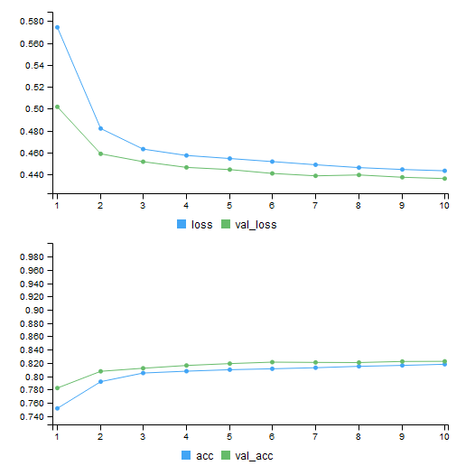
If a split ratio or validation set was assigned, loss and the fitness metrics will not only be displayed for the training (blue line) set but also for the validation set (green line). A graph like this is very useful to identify problems that may occur during training. If the model gets stuck someplace or becomes overtrained, this graph will tell you.

As Figure 8.6 suggests, training has gone smoothly. Training and validation metrics are pretty close together. If the training loss was going down while the validation loss was going up, that would be a sign of overtraining. The model would be so addicted to the training set that it would fail to generalize well into as-yet-unseen data.

Luckily, that was not what happened. If that was the case, there would be things to do: lowering the learning ratio, using fewer epochs, using dropout or other regularization techniques. More on that later, but for the time being, let's move to the evaluation phase. To evaluate a model, we pipe the evaluate()  method to the network:

heracles_1 %>% evaluate(train_dt, train_target)
# 25000/25000 ...
# $loss
# [1] 0.4409437
# 
# $acc
# [1] 0.817

A progression bar will be outputted with it. Inside the evaluate() method, input the model's input and output. Using the training data, the model showed 81.7% accuracy:

heracles_1 %>% evaluate(val_dt, val_target)
# 5000/5000 ...
# $loss
# [1] 0.4362364
#
# $acc
# [1] 0.8224

The model performed slightly better with the validation data. Accuracy reached 82,24%. Is that a good mark? To answer such a question, benchmarks must be established. Since credit card defaults aren't supposed to be that common, we could compare the accuracy with the proportion of non-defaults.

This way, we make sure that our model is not guessing no default every time. Given that default was encoded using one hot, we can use mean() to compute the proportion of non-default:

mean(train_target[,1])
# [1] 0.77812
mean(val_target[,1])
# [1] 0.7822

The network did better than simply guessing no default all the time. Another thing we can see from that is how unbalanced the dataset is. Although this data was pretty unbalanced, it did not negatively affect the network. If it does, there is a pretty cool way to solve that. It consists of changing the weight of the class that shows up the least so that missing that class will cost more.

I would say that heracles_1 did a very good job, and it's worth saving. There is a specific function to save Keras's models:

save_model_hdf5(heracles_1, filepath = 'heracles_1.hdf5',
                overwrite = T, include_optimizer = T)

We could make heracles_1 vanish:

rm(heracles_1)

And we could load it again using load_model_hdf5():

heracles_1 <- load_model_hdf5(filepath = 'heracles_1.hdf5')

But what if heracles_1 had overfitted a lot? I would try to use dropout. What if it had struggled a lot to learn? I would try Leaky ReLU. The next code block shows how to use dropout and to use Leaky ReLU rather than the regular ReLU:

heracles_2 <- keras_model_sequential() %>% 
  layer_dense(units = 25, input_shape = 33) %>%
  layer_activation_leaky_relu(alpha = .3) %>% 
  layer_dropout(rate = .2) %>% 
  layer_dense(units = 15) %>%
  layer_activation_leaky_relu(alpha = .3) %>% 
  layer_dropout(rate = .1) %>% 
  layer_dense(units = 6) %>% 
  layer_activation_leaky_relu(alpha = .3) %>% 
  layer_dropout(rate = .05) %>% 
  layer_dense(units = 2, activation = 'softmax')

To adopt Leaky ReLU, we suppressed the activation argument inside layer_dense() and piped layer_activation_leaky_relu() right next to layer_dense(). Notice the argument alpha. It's a very important parameter for Leaky ReLU—regular ReLU can be seen as a Leaky ReLU with alpha set to zero.

To use dropout in a layer, we simply have to pipe layer_dropout(). Do not forget to assign the rate argument inside it. It must range between zero and one. Layers with more units can afford a greater dropout ratio, while layers with fewer units should have it closer to zero. This discussed how to design, train, evaluate, save, and load a model using Keras.