R contains inbuilt functions for reading data. The most commonly used format is CSV, that is, CSV files. There are multiple commands to read CSV files. A few are shown as follows. In order to conduct our tests, we will use the mtcars dataset in R.

First, we are going to create a copy of the dataset into a new variable called car_data:

car_data <- mtcars 

To view the top few rows of the mtcars dataset, we can use the head command. This is often very useful in getting a quick glimpse of the data we will be working with:

head(car_data) 

The following is the output of the preceding code:

Create the CSV file:

write.csv(car_data,"car_data.csv") 
fwrite(car_data, "car_data.csv") 

We can view the file that was saved in the current directory:

list.files(".", pattern = "car_data*") 
# [1] "car_data.csv" 
 
# Reading the CSV file 
read.csv("car_data.csv") # Base R 
read_csv("car_data.csv") # Tidyverse 
fread("car_data.csv")   # data.table 

While these are mostly similar, note that the output is slightly different. The first one, read.csv, is from base R (it comes inbuilt in R) and creates data.frame. The second, read_csv, is from the tidyverse package and creates tibble as discussed in Chapter 3, Data Wrangling with R. The third option, fread, produces data.table, which has different characteristics compared to data.frame, but is arguably much faster in reading large amounts of data.

Once you have read the file, the next step is to see what the data contains and the respective data types. This can be done using the str command in R. The command, str stands for structure and provides a summarized overview of the data types:

# To view data type and first few records 
str(read.csv("car_data.csv"))     # Base R 
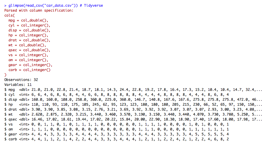
glimpse(read_csv("car_data.csv")) # Tidyverse 

The output of the preceding code is as follows: