15

Taming Data with Tableau Prep

We considered some options for structuring data in Tableau Desktop in the previous chapter. Many of the concepts around well-structured data will apply here as we now turn our attention to another product from Tableau: Tableau Prep. Tableau Prep extends the Tableau platform with robust options for cleaning and structuring data for analysis in Tableau. In the same way that Tableau Desktop provides a hands-on, visual experience for visualizing and analyzing data, Tableau Prep provides a hands-on, visual experience for cleaning and shaping data.

Tableau Prep is on an accelerated, monthly release cycle and while the platform continues to grow and expand, there is an underlying paradigm that sets a foundation for cleaning and shaping data. We'll cover a lot of ground in this chapter, but our goal is not to cover every possible feature—and indeed, we won't. Instead, we will seek to understand the underlying paradigm and flow of thought that will enable you to tackle a multitude of data challenges in Tableau Prep.

In this chapter, we'll work through a couple of practical examples as we explore the paradigm of Tableau Prep, understand the fundamental transformations, and see many of the features and functions of Tableau Prep.

We'll cover quite a few topics in this chapter, including the following:

• Getting ready to explore Tableau Prep
• Understanding the Tableau Prep Builder interface
• Flowing with the fundamental paradigm
  • Connecting to data
  • Cleaning the data
  • Calculations and aggregations in Tableau Prep
  • Filtering data in Tableau Prep
  • Transforming the data for analysis
• Options for automating flows

In this chapter, we'll use the term Tableau Prep broadly to speak of the entire platform that Tableau has developed for data prep and sometimes as shorthand for Tableau Prep Builder, the client application that's used to connect to data, create data flows, and define output. Where needed for clarity, we'll use these specific names:

• Tableau Prep Builder: The client application that's used to design data flows, run them locally, and publish them
• Tableau Prep Conductor: An add-on to Tableau Server that allows the scheduling and automation of published data flows

Let's start by understanding how to get started with Tableau Prep.

Getting ready to explore Tableau Prep

Tableau Prep Builder is available for Windows and Mac. If you do not currently have Tableau Prep Builder installed on your machine, please take a moment to download the application from https://www.tableau.com/products/prep/download. Licenses for Tableau Prep Builder are included with Tableau Creator licensing. If you do not currently have a license, you may trial the application for 14 days. Please speak with your Tableau representative to confirm licensing and trial periods.

The examples in this chapter use files located in the Learning TableauChapter 15 directory. Specific instructions will guide you on when and how to use the various files.

Once you've downloaded and installed Tableau Prep Builder, you will be able to launch the application. Once you do, you'll find a welcome screen that we'll detail as we cover the interface in the next section.

Understanding the Tableau Prep Builder interface

You'll find a lot of similarities in the interfaces of Tableau Prep Builder and Tableau Desktop. The home screen of Tableau Prep Builder will look similar to this:

Figure 15.1: The Tableau Prep Builder welcome screen with numbering to identify key components of the UI

The following components have been numbered in Figure 15.1:

1. The menu includes options for opening files, editing and running flows, signing into Tableau Server, and various Help functions. Also notice the Connections Pane to the left, immediately beneath the File menu. It is collapsed initially, but will contain a list of data connections as you create them.
2. The two large buttons at the top give you the option to Open a Flow, which opens an existing Tableau Prep flow file, or Connect to Data, to start a new flow with an initial data connection. We'll define a flow in the next section. For now, think of a flow in terms of Tableau Prep's equivalent of a Tableau Desktop workbook.
3. Recent Flows shows the Tableau Prep data flows that you have recently saved. You may click on one of these to open the flow and edit or run it. A toggle button on the right allows you to switch between thumbnails and a list.
4. Sample Flows allows you to open some prebuilt examples.
5. The Discover pane gives you options for training and resources as you learn more about Tableau Prep. A notification to upgrade will also appear if there is a newer version available.

Once you have opened or started a new flow, the home screen will be replaced with a new interface, which will facilitate the designing and running of flows:

Figure 15.2: When designing a flow, you'll find an interface like this one. The major components are numbered and described as follows

This interface consists of the following, which are numbered in the preceding screenshot:

1. The flow pane, where you will logically build the flow of data with steps that will do anything from cleaning to calculation, to transformation and reshaping. Selecting any single step will reveal the interface on the bottom half of the screen. This interface will vary slightly, depending on the type of step you have selected.
2. The settings, or changes pane lists settings for the step and also a list of all changes that are made in the step, from calculations to renaming or removing fields, to changing data types or grouping values. You can click on individual changes to edit them or see how they alter the data.
3. The profile pane gives you a profile of each field in the data as it exists for the selected step. You can see the type and distribution of values for each field. Clicking on a field will highlight the lineage in the flow pane and clicking one or more values of a field will highlight the related values of other fields.
4. The data grid shows individual records of data as they exist in that step. Selecting a change in the changes grid will show the data based on changes up to and including the selected change. Selecting a value in the profile pane will filter the data grid to only show records containing that value. For example, selecting the first row of the Order Date field in the profile pane will filter the data grid to show only records represented by that bar. This allows you to explore the data, but doesn't alter the data until you perform a specific action that does result in a change.

You will also notice the toolbar that allows you to undo or redo actions, refresh data, or run the flow. Additionally, there will be other options or controls that appear based on the type of step or field that's selected. We'll consider those details as we dive into the paradigm of Tableau Prep, and a practical example later in the chapter.

Flowing with the fundamental paradigm

The overall paradigm of Tableau Prep is a hands-on, visual experience of discovering, cleaning, and shaping data through a flow. A flow (sometimes also called a data flow) is a logical series of steps and changes that are applied to data from input(s) to output(s).

Here is an example of what a flow looks like in the flow pane of Tableau Prep:

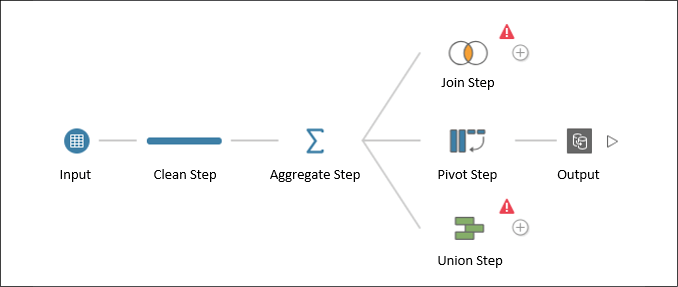
Figure 15.3: An example flow in Tableau Prep

Each of the individual components of the flow are called steps, which are connected by lines that indicate the logical flow of data from left to right. The lines are sometimes called connectors or branches of the flow. Notice that the Aggregate Step here has one line coming in from the left and three branches extending to the right. Any step can have multiple output branches that represent logical copies of the data at that point in the flow.

One important thing to notice is that four of the step types represent the four major transformations of data we discussed in Chapter 14, Structuring Messy Data to Work Well in Tableau. The step types of Pivot, Union, Join, and Aggregate exactly match those transformations, while the Clean Step allows various other operations involved in cleaning and calculating. You may wish to refresh your memory on the basic transformations in the previous chapter.

As we work through an example of a flow throughout this chapter, we'll examine each type of step more closely. For now, consider these preliminary definitions of the primary steps in Tableau Prep:

• Input: An input step starts the flow with data from a source such as a file, table, view, or custom SQL. It gives options for defining file delimiters, unions of multiple tables or files, and how much data to sample (for larger record sets).
• Clean Step: A clean step allows you to perform a wide variety of functions on the data, including calculations, filtering, adjusting data types, removing and merging fields, grouping and cleaning, and much more.
• Aggregate Step: An aggregate step allows you to aggregate values (for example, get MIN, MAX, SUM, AVG) at a level of detail you specify.
• Join Step: A join step allows you to bring together two branches of the flow and match data row by row based on the fields you select and the type of join.
• Union Step: A union step allows you to bring together two or more branches representing sets of data to be unioned together. You will have options for merging or removing mismatched fields.

  Both the Union Step and Join Step in this example have an error icon, indicating that something has not been configured correctly in the flow. Hovering over the icon gives a tooltip description of the error. In this case, the error is due to only having one input connection, while both the union and join require at least two inputs. Often, selecting a step with an error icon may reveal details about the error in the changes pane or elsewhere in the configuration steps.

• Pivot Step: A pivot step allows you to transform columns of data into rows or rows of data into columns. You'll have options to select the type of pivot as well as the fields themselves. The term transpose is sometimes also used to describe this operation.
• Output: The output step defines the ultimate destination for the cleaned and transformed data. This could be a text file (.csv), extract (.hyper or .tde), or published extracted data source to Tableau Server. The ability to output to a database has been announced, although is not available at the time of writing. You'll have options to select the type of output, along with the path and filename or Tableau Server and project.

In addition to using the term flow to refer to the steps and connections that define the logical flow and transformation of the data, we'll also use the term flow to refer to the file that Tableau Prep uses to store the definition of the steps and changes of a flow. Tableau Prep flow files have the .tfl (unpackaged flow) or .tflx (packaged flow) extension.

The paradigm of Tableau Prep goes far beyond the features and capabilities of any single step. As you build and modify flows, you'll receive instant feedback so that you can see the impact of each step and change. This makes it relatively easy (and fun!) to iteratively discover your data and make the necessary changes.

We'll consider an example in the remainder of this chapter to aid in our discussion of the Tableau Prep paradigm and highlight some important features and considerations. The example will unfold organically, which will allow us to see how Tableau Prep gives you incredible flexibility to address data challenges as they arise and make changes as you discover new aspects of your data.

We'll put you in the role of an analyst at your organization, with the task of analyzing employee air travel. This will include ticket prices, airlines, and even a bit of geospatial analysis of the trips themselves. The data needs to be consolidated from multiple systems and will require some cleaning and shaping to enable the analysis.

To follow along, open Tableau Prep Builder, which will start on the home screen (there is not a starter flow for this chapter). The sample data is in the Chapter 15 directory, along with the Complete flow if you want to check your work. The Complete (clean) flow contains a sample of how a flow might be self-documented—it will not match screenshots precisely.

We'll start by connecting to some data!

Connecting to data

Connecting to data in Tableau Prep is very similar to connecting to data in Tableau Desktop. From the home screen, you may click either Connect to Data or the + button on the expanded Connections pane:

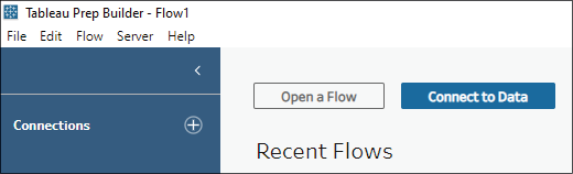
Figure 15.4: You can make a new data connection by clicking the + button or the Connect to Data button

Either UI element will bring up a list of data source types to select.

Tableau Prep supports dozens of file types and databases, and the list continues to grow. You'll recognize many of the same types of connection possibilities that exist in Tableau Desktop. However, at the time of writing this book, Tableau Prep does not support all the connections that are available in Tableau Desktop.

You may create as many connections as you like and the Connections pane will list each connection separately with any associated files, tables, views, and stored procedures, or other options that are applicable to that data source. You will be able to use any combination of data sources in the flow.

For now, let's start our example with the following steps:

1. Starting from the window shown in Figure 15.4, click Connect to Data.
2. From the expanded list of possible connections that appears, select Microsoft Excel.
3. You'll see a main table called Employee Flights and a sub-table named Employee Flights Table 1. Drag the Employee Flights table to the flow canvas. An input step will be created, giving you a preview of the data and other options. The input preview pane will initially look like this:

   

   Figure 15.5: The input preview allows you to select input fields to include in the flow, rename fields, and change data types

   The input step displays a grid of fields and options for those fields. You'll notice that many of the fields in the Employee Flights table are named F2, F3, F4, and so on. This is due to the format of the Excel file, which has merged cells and a summary sub-table. Continue the exercise with the following steps:

4. Check the Use Data Interpreter option on the Connections pane and Tableau Prep will correctly parse the file as shown here:

   

   Figure 15.6: The data interpreter parses the file to fix common issues such as merged cells, empty headers, and sub-total lines

   When you select an input step, Tableau Prep will display a grid of fields in the data. You may use the grid to uncheck any fields you do not wish to include, edit the Type of data by clicking the associated symbol (for example, change a string to a date), and edit the Field Name itself by double-clicking the field name value.

   If Tableau Prep Builder detects that the data source contains a large number of records, it may turn on data sampling. Data Sampling uses a smaller subset of records for giving rapid feedback and profiling in design mode. However, it will use the full set of data when you run the entire flow in batch mode. You can control the data sampling options by clicking Data Sample on the input pane. While you can set the sample size for the source, subsequent steps, such as joins, that result in large numbers of records may turn on sampling that cannot be disabled. You'll receive an indicator of Data Sampling if it occurs anywhere in the flow.

5. Now, we'll continue to explore the data and fix some issues along the way. Click the + button that appears when you hover over the Employee Flights input step. This allows you to extend the flow by adding additional step types. In this case, we'll add a Clean Step. This will extend the flow by adding a clean step called Clean 1:

   

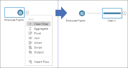
   Figure 15.7: Adding a step extends the flow. Here, adding a clean step adds Clean 1

6. With the Clean 1 step selected, take a moment to explore the data using the profile pane. Observe how selecting individual values for fields in the profile pane highlights portions of related values for other fields. This can give you great insight into your data, such as seeing the different price ranges based on Ticket Type:

   

   Figure 15.8: Selecting a value for a field in the profile pane highlights which values (and what proportion of those values) relate to the selected value

Highlighting the bar segments across fields in the profile pane, which results from selecting a field value, is called brushing. You can also take action on selected values via the toolbar at the top of the profile pane or by right-clicking a field value. These actions include filtering, editing values, or replacing with NULL. However, before making any changes or cleaning any of the data, let's connect to some additional data.

It turns out that most of the airline ticket booking data is in one database that's represented by the Excel file, but another airline's booking data is stored in files that are periodically added to a directory. These files are in the Learning TableauChapter 15 directory. The files are named with the convention Southwest YYYY.csv (where YYYY represents the year).

We'll connect to all the existing files and ensure that we are prepared for additional future files:

1. Click the + icon on the connections pane to add a new connection to a Text File.
2. Navigate to the Learning TableauChapter 15 directory and select any of the Southwest YYYY.csv files to start the connection. Looking at the Input settings, you should see that Tableau Prep correctly identifies the field separators, field names, and types: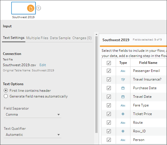

   

   Figure 15.9: A text file includes options for headers, field separators, text qualifiers, character sets, and more. Notice also the tabs such as Multiple Files and Data Sample giving other options for the text input

3. In the Input pane, select the Multiple Files tab and switch from Single table to Wildcard union. Set Matching Pattern to Southwest* and click Apply. This tells Tableau Prep to union all of the text files in the directory that begin with Southwest together:

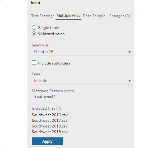
Figure 15.10: Using Matching Pattern tells Tableau Prep which files to union together. That way, when Southwest 2020.txt and future files are dropped into the directory, they will be automatically included

4. Use the + icon on the Southwest input step in the flow pane to add a new clean step. This step will be named Clean 2 by default. Once again, explore the data, but don't take any action until you've brought the two sources together in the flow. You may notice a new field in the Clean 2 step called File Paths, which indicates which file in the union is associated with each record.

With our input steps defined, let's move on to consider how to clean up some of the data to get it ready for analysis.

Cleaning the data

The process of building out the flow is quite iterative, and you'll often make discoveries about the data that will aid you in cleaning and transforming it. We'll break this example into sections for the sake of reference, but don't let this detract from the idea that building a flow should be a flow of thought. The example is meant to be seamless!

We'll take a look at quite a few possibilities for prepping the data in this section, including merging and grouping. Let's start with seeing how to union together branches in the flow.

Unioning, merging mismatched fields, and removing unnecessary fields

We know that we want to bring together the booking data for all the airlines, so we'll union together the two paths in the flow:

1. Drag the Clean 2 step onto the Clean 1 step and drop it onto the Union box that appears. This will create a new Union step with input connections from both of the clean steps:

   

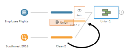
   Figure 15.11: Dragging one step onto another in the flow reveals options for bringing the datasets together in the flow. Here, for example, there are options for creating a Union or Join

2. The Union pane that shows up when the Union step is selected will show you the mismatched fields, indicate the associated input, and give you options for removing or merging the fields. For example, Fare Type and Ticket Type are named differently between the Excel file and the text files, but in fact represent the same data. Hold down the Ctrl key and select both fields. Then, select Merge Fields from the toolbar at the top of the pane or from the right-click menu: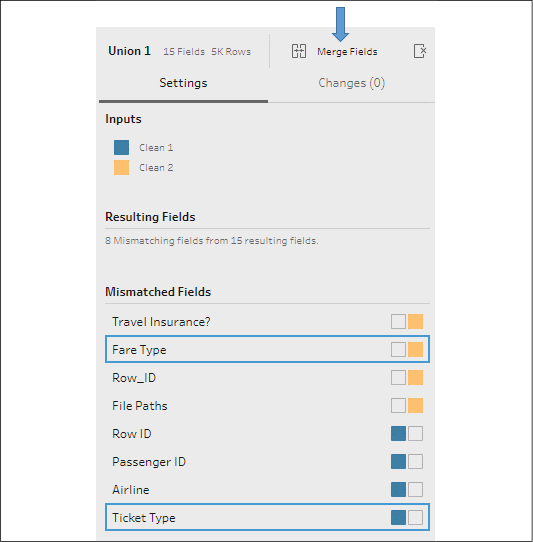

   

   Figure 15.12: When you select a single field, Tableau Prep will highlight fields that are potentially the same data. Selecting both reveals the Merge Fields option

3. Also, merge Row ID and Row_ID.
4. File Paths applies only to the Southwest files, which were unioned together in the Input step. While this auto-generated field can be very useful at times, it does not add anything to the data in this example. Select the field, then click the ellipses menu button and select Remove Field.
5. Similarly, Travel Insurance? and Passenger ID apply to only one of the inputs and will be of little use in our analysis. Remove those fields as well.

6. The single remaining mismatched field, Airline, is useful. Leave it for now and click the + icon on the Union 1 step in the flow pane and extend the flow by selecting Clean Step. At this point, your flow should look like this:

   

   Figure 15.13: Your flow should look similar to this. You may notice some variation in the exact location of steps or color (you can change a step's color by right-clicking a step)

Next, we'll continue building the flow and consider some options for grouping and cleaning.

Grouping and cleaning

Now, we'll spend some time cleaning up the data that came from both input sources. With the Clean 3 step selected, use the profile pane to examine the data and continue our flow. The first two fields indicate some issues that need to be addressed:

Figure 15.14: Every null value in the Airline field comes from the Southwest files. Fortunately, in this case, the source of the data indicates the airline

The Table Names field was generated by Tableau Prep as part of Union 1 to indicate the source of the records. The Airline field came only from the Excel files (you can confirm this by selecting it in the profile pane and observing the highlighted path of the field in the flow pane). Click the null value for Airline and observe the brushing: this is proof that the null values in Airline all come from the Southwest files since those files did not contain a field to indicate the airline. We'll address the null values and do some additional cleanup:

1. Double-click the null value and then type Southwest to replace NULL with the value you know represents the correct airline. Tableau Prep will indicate that a Group and Replace operation has occurred with a paperclip icon.
2. We'll do an additional grouping to clean up the variations of American. Using the Options button on the Airline field, select Group Values | Pronunciation: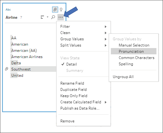

   

   Figure 15.15: The ellipses button on a field will reveal a plethora of options, from cleaning to filtering, to grouping, to creating calculations

   Nearly all the variations are grouped into the American value. Only AA remains.

3. In the Group Values by Pronunciation pane that has appeared, select the American Airlines group and manually add AA by checking it in the list that appears to the right:

   

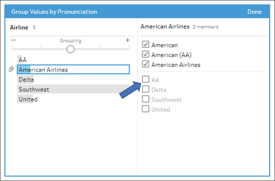
   Figure 15.16: When grouping by pronunciation, you'll notice a slider allowing you control over the sensitivity of the grouping. You can also manually adjust groupings by selecting a field

4. Click Done on the Group Values by Pronunciation pane.
5. Next, select the Table Names field, which is no longer needed. Using either the toolbar option, the menu from a right-click for the field, or the options button, select Remove Field.
6. Some fields in the profile pane have a Recommendations icon (which resembles a lightbulb) in the upper-right corner. Click this icon on the Passenger Email field and then Apply the recommendation to assign a data role of Email: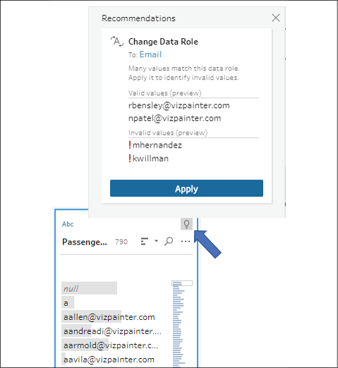

   

   Figure 15.17: Recommendations will show when Tableau Prep has suggestions for cleaning a field

   Data Roles allow you to quickly identify valid or invalid values according to what pattern or domain of values is expected. Once you have assigned a data role, you may receive additional recommendations to either filter or replace invalid values.

   After applying the recommendation, you'll see an indication in the profile pane for invalid values. As you continue following the example, we'll consider some options for quickly dealing with those invalid values.

7. Click the Recommendations button on the Passenger Email field again. You'll see two new options presented. Apply the option to Group and Replace invalid values with null: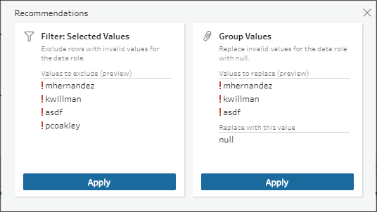

   

   Figure 15.18: Here, Tableau Prep suggests either filtering out records with invalid values or replacing the invalid values with null. In this case, we don't want to filter out the entire record, but the invalid values themselves are useless and are best represented by null

8. Most of the remaining fields look fine, except for Fare Type (or possibly Ticket Type, depending on which name was kept when merging the fields previously). This field contains the values 1st Class and First Class. Select both of these values by clicking each while holding down the Ctrl key and then Group them together with the First Class value. Two interface options for grouping the values are indicated here:

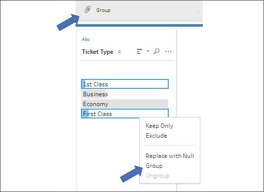
Figure 15.19: After selecting two or more values, you can group them together with the toolbar option or the right-click menu

9. At this point, we have a clean dataset that contains all our primary data. There's already a lot of analysis we could do. In fact, let's take a moment to preview the data. Right-click the Clean 3 step and select Preview in Tableau Desktop:

   

   Figure 15.20: You may preview the data represented by any step in Tableau Desktop by selecting the option from the right-click menu for that step

A new data connection will be made and opened in Tableau Desktop. You can preview the data for any step in the flow. Take a few moments to explore the data in Tableau Desktop and then return to Tableau Prep. Now, we'll turn our attention to extending the dataset with some calculations, supplemental data, and a little restructuring.

Calculations and aggregations in Tableau Prep

Let's look at how to create calculations and some options for aggregations in Tableau Prep.

Row-level calculations

Calculations in Tableau Prep follow a syntax that's nearly identical to Tableau Desktop. However, you'll notice that only row-level and FIXED level of detail functions are available. This is because all calculations in Tableau Prep will apply to the row level. Aggregations are performed using an Aggregate Step, which we'll consider shortly.

Calculations and aggregations can greatly extend our analytic capabilities. In our current example, there is an opportunity to analyze the length of time between ticket purchase and actual travel. We may also want to mark each record with an indicator of how frequently a passenger travels overall. Let's dive into these calculations as we continue our example with the following steps:

1. We'll start with a calculation to determine the length of time between the purchasing of tickets and the day of travel. Select the Clean 3 step and then click Create Calculated Field. Name the calculation Days from Purchase to Travel and enter DATEDIFF('day', [Purchase Date], [Travel Date]).
2. Examine the results in the profile pane. The new field should look like this:

   

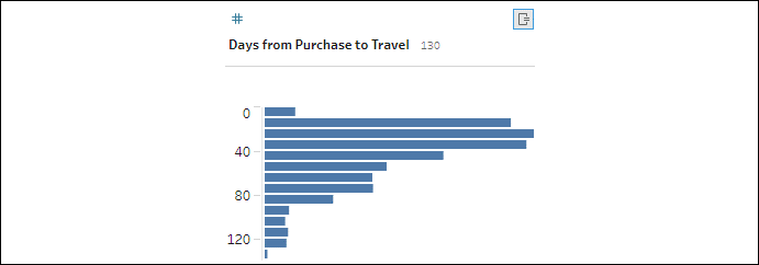
   Figure 15.21: The calculated field shows up in the profile pane

The default view here (as in many cases with numeric fields) is a summary binned histogram. You can change the view to see its details by selecting the ellipses button in the upper right of the field and switching to Detail, which will show every value of the field:

Figure 15.22: Numeric and date fields can be viewed in Summary or in Detail

The shape of the data that's indicated by the default summary histogram is close to what we might have expected with most people purchasing tickets closer (but not immediately prior) to the date of travel. There might be some opportunity for getting better deals by purchasing farther in advance, so identifying this pattern (and then exploring it more fully in Tableau Desktop) will be key for this kind of analysis.

Level of detail calculations

There are a few other types of analysis we may wish to pursue. Let's consider how we might create segments of passengers based on how often they travel.

We'll accomplish this using a FIXED level of detail (LOD) expression. We could create the calculation from scratch, matching the syntax we learned for Tableau Desktop to write the calculation like this:

{FIXED [Person] : COUNTD([Row_ID])}

The preceding calculation would count the distinct rows per person. Knowing that each row represents a trip, we could alternately use the code {FIXED [Person] : SUM(1)}, which would potentially be more performant, depending on the exact data source.

In this example, though, we'll leverage the interface to visually create the calculation:

1. Click the ellipses button on the Person field and select Create Calculated Field | Fixed LOD:

   

   Figure 15.23: To create a Fixed LOD calculation, use the menu and select Create Calculated Field | Fixed LOD

   Notice also the options to create Custom Calculation (to write code) and Rank (to compute rank for the selected field).

2. This will bring up a Fixed LOD pane allowing us to configure the LOD expression. The Group by field is already set to Person (as we started the calculation from that field), but we'll need to configure Compute using to perform the distinct count of rows and rename the field as Trips per Person, as shown here:

   

   Figure 15.24: The Fixed LOD pane allows you to configure the LOD expression visually and get instant visual feedback concerning results

3. Click Done when you have finished configuring the Fixed LOD.
4. We'll use the Trips per Person field to create segments of customers. We'll accomplish this with another calculated field, so click Create Calculated Field… to bring up the code editor. Name the field Frequency Segment and enter the following code:

   IF [Trips per Person] <= 2 THEN "Rarely"
   ELSEIF [Trips per Person] <= 5 THEN "Occasionally"
   ELSE "Frequently"
   END
   

The code uses the Trips per Person field in an If Then Else construction to create three segments. You can visually see the correspondence between the fields in the preview pane:

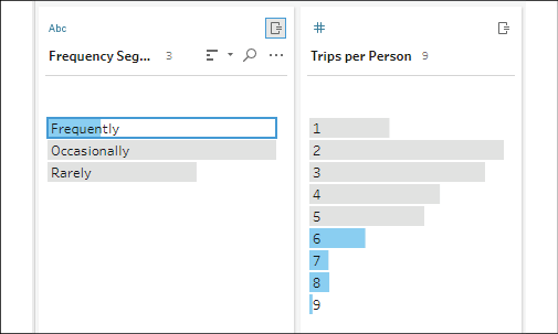
Figure 15.25: You can easily visualize how calculations relate to each other and other fields using the Profile pane

The Frequency Segment field can be used to accomplish all kinds of useful analysis. For example, you might want to understand whether frequent travelers typically get better ticket prices.

We've seen row-level and FIXED LOD calculations, and noted the option for Rank. Let's now turn our attention to aggregations.

Aggregations

Aggregations in Tableau Prep are accomplished using an aggregate step. We'll continue our flow with the idea that we want to better understand our frequency of travel segment:

1. Click the + symbol on Clean 3 and add an Aggregate step. The new step will be named Aggregate 1 by default:

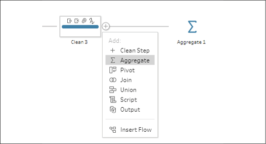
Figure 15.26: Adding an Aggregate step to the flow using the + symbol

2. Double-click the text Aggregate 1 under the new step. This allows you to edit the name. Change the name from Aggregate 1 to Frequency Segment.

   Give steps meaningful names to self-document the flow. This will greatly help you and others when you return to edit the flow in the future. Additionally, when you are editing the name of a step, the Add a description text will appear below the name, as shown in Figure 15.27.

   

   Figure 15.27: When editing the name of a step, you may also add a more verbose description to help document the steps purpose

   Selecting the aggregate step reveals a pane with options for grouping and aggregating fields in the flow:

   

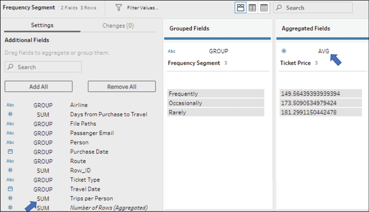
   Figure 15.28: Adding an Aggregate step to the flow using the + symbol

   You may drag and drop fields from the left to the Grouped Fields or Aggregated Fields sections and you may change the type of aggregation by clicking on the aggregation text (examples indicated by arrows in Figure 15.28: SUM next to Trips per Person or AVG above Ticket Price) and selecting a different aggregation from the resulting dropdown.

   In Figure 15.28, notice that we've added Frequency Segment to the GROUP and Ticket Price to the Aggregated Fields as an AVG. Notice also the Number of Rows (Aggregated) that appears at the bottom of the list of fields on the left. This is a special field that's available in the aggregation step.

3. Conclude the example by clicking the + icon that appears when you hover over the Frequency Segment aggregate step and adding an Output step:

   

   Figure 15.29 Adding an Output step to the flow using the + symbol

4. When you select the Output step, the Output pane shows options for saving the output and a preview of what the output will look like. In this case, we've configured the output to save to a Comma Separated Values (.csv) file named Frequency Segment:

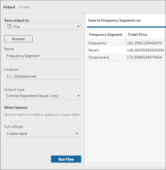
Figure 15.30: This output will contain exactly three rows of data

5. The Output pane also gives options for setting the output type, performing a full refresh of the data, or appending to existing data, and running the flow.

We'll extend our flow in the next few sections to additionally output detailed data. The detailed data as well as the output file of aggregate data gives us some nice options for leveraging Tableau's Data Model in Tableau Desktop to accomplish some complex analysis.

Let's continue by thinking about filtering data in Tableau Prep.

Filtering data in Tableau Prep

There are a couple of ways to filter data in Tableau Prep:

• Filter an input
• Filter within the flow

Filtering an input can be efficient because the query that's sent to the data source will return fewer records. To filter an input, select the input step and then click the Filter Values... button on the input pane:

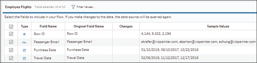
Figure 15.31: The Filter Values... option allows you to filter values on the input step. This could improve performance on large datasets or relational databases

The Add Filter dialog that pops up allows you to write a calculation with a Boolean (true/false) result. Only true values will be retained.

Filtering may also be done within a clean step anywhere in the flow. There are several ways to apply a filter:

• Select one or more values for a given field and then use the Keep Only or Exclude options.
• Use the Option button on a field to reveal multiple filter options based on the field type. For example, dates may be filtered by Calculation…, Range of Dates, Relative Dates, or Null Values:

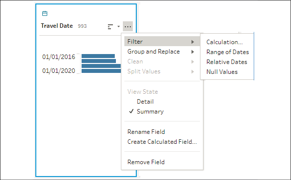
Figure 15.32: Filter options for a field include filtering by Calculation, Range of Dates, and Relative Dates, and keeping or excluding Null Values

• Select a field and then Filter Values from the toolbar. Similar to the way filters work in the input pane, you will be prompted to write code that returns true for records you wish to keep. If, for example, you wanted to keep records for trips scheduled after January 1, 2016, you could write code such as the following:

  [Travel Date] > MAKEDATE(2016, 1, 1) 
  

While no filtering is required for the dataset in our example, you may wish to experiment with various filtering techniques.

At this point, your flow should look something like this:

Figure 15.33: Your flow should look similar to this (exact placement and colors of steps may vary)

Let's conclude the Tableau Prep flow with some final transformations to make the data even easier to use in Tableau.

Transforming the data for analysis

Let's create a new branch in the flow to work once again with the detailed data. Click on the Clean 3 step and examine the preview pane. In particular, consider the Route field:

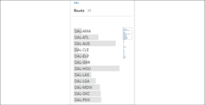
Figure 15.34: Route uses airport codes for origin and destination separated by a dash

Tableau Desktop (and Server) contain built-in geocoding for airport codes. But to accomplish our specific analysis goal (and open other possibilities for geospatial functions in Tableau Desktop), we'll supplement our data with our own geocoding. We'll also need to consider the shape of the data. Origins and destinations will be most useful split into separate fields, and if we want to connect them visually, we'll also want to consider splitting them into separate rows (a row for the origin and another row for the destination).

If you are following along, here are the steps we'll take:

1. Use the + button that appears when you hover over the Clean 3 step. Use that to add a new clean step, which will be automatically named Clean 4:

   

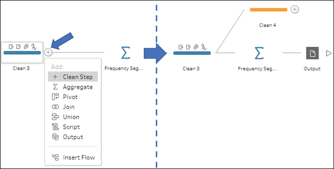
   Figure 15.35: Adding to a step that already has an output adds a new branch to the flow

2. In the Clean 4 step, use the ellipses button on the Route field and select Split Values | Automatic Split: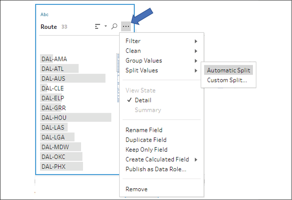

   

   Figure 15.36: Split Values allows you to divide delimited strings into separate fields. Automatic Split attempts to determine the delimiter, while Custom Split… allows you greater options and flexibility

   You'll now see two new fields added to the step:

   

   Figure 15.37: The results of the split will be new fields in the flow

3. Route - Split 1 is the origin and Route - Split 2 is the destination. Double-click the field name in the profile pane (or use the option from the ellipses button) to rename the fields to Origin and Destination.
4. Locate the US Airports.hyper file in the Chapter 15 directory. This file contains each Airport Code along with the Airport Name and Latitude and Longitude: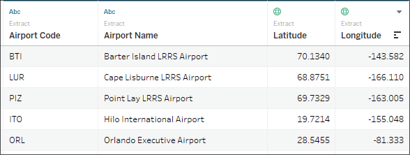

   

   Figure 15.38: The hyper extract contains the data we'll need to supplement the flow with our own geospatial data

5. Make a connection to this file in Tableau Prep. You may choose to drag and drop the file onto the Tableau Prep canvas or use the Add Connection button from the interface. Tableau will automatically insert an input step named Extract (Extract.Extract). Feel free to change the name of the input step to Airport Codes:

   

   Figure 15.39: The input pane for the Airport Codes file

6. We'll want to join the Airport Codes into our flow to look up Latitude and Longitude, but before we do, we'll need to account for the fact that Origin and Destination in Clean 4 are currently both on the same row of data. One option is to pivot the data. Use the + button on the Clean 4 step to add a Pivot step: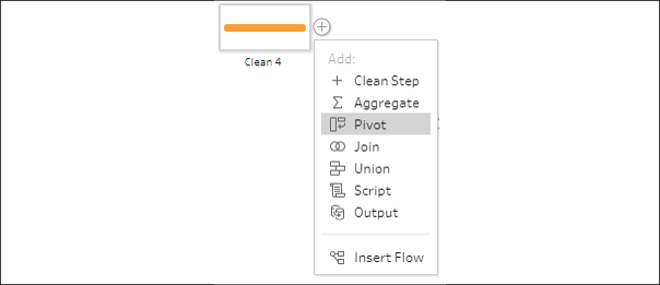

   

   Figure 15.40: Adding a Pivot step from Clean 4

7. The pivot pane gives you options for transforming rows into columns or columns into rows. We'll keep the default option of Columns to Rows. Drag both the Origin and Destination fields into the Pivot1 Values area of the pane: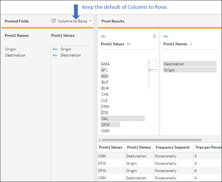

   

   Figure 15.41: Pivot1 Names keeps values from the original column names, while Pivot1 Values contains the actual values from Origin and Destination

8. As a shortcut, instead of steps 6 and 7, you could have selected both the Origin and Destination fields in the Clean 4 step, and selected Pivot Columns to Rows:

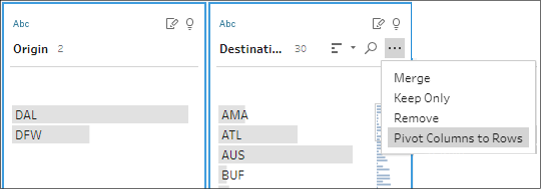
Figure 15.42: A shortcut for pivoting columns to rows

Continue with the following steps:

9. Double-click the text for Pivot1 Values and rename the field Airport Code. This field will contain all the airport codes for both the origin and destination records.
10. Double-click the text for Pivot1 Names and rename the field Route Point. This field will label each record as either an Origin or Destination.

    At this point, we have a dataset that contains a single record for each endpoint of the trip (either an origin or destination).

    Notice that the pivot resulted in duplicate data. What was once one row (origin and destination together) is now two rows. The record count has doubled, so we can no longer count the number of records to determine the number of trips. We also cannot SUM the cost of a ticket as it will double count the ticket. We'll need to use MIN/MAX/AVG or some kind of level of detail expression or filter to look at only origins or destinations. While many transformations allow us to accomplish certain goals, we have to be aware that they may introduce other complications.

    The only location information we currently have in our main flow is the airport code. However, we already made a connection to Airports.hyper and renamed the input step as Airport Codes.

11. Locate the Airport Codes input step and drag it over the Pivot step. Drop it onto the Join area:

    

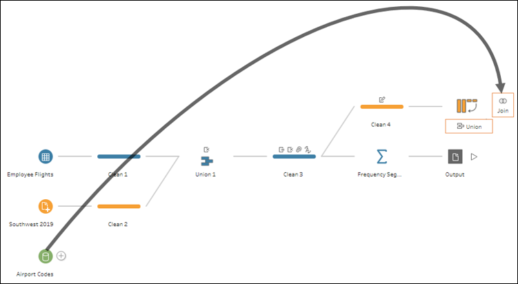
    Figure 15.43: Dragging Airport Codes to the Join area of the Pivot step

    After dropping the Airport Codes input step onto the Join area, a new join step will be created, named Join 1. Take a moment to examine the join pane:

    

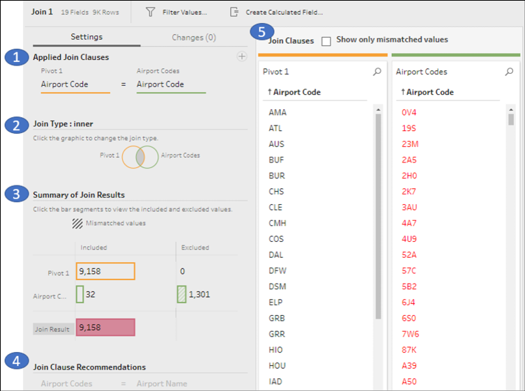
    Figure 15.44: The join pane gives a lot of information and options for configuring the join and understanding the results. Important sections of the interface are numbered with descriptions below

You'll notice the following features in Figure 15.44:

1. Applied Join Clauses: Here, you have the option to add conditions to the join clause, deciding which fields should be used as keys to define the join. You may add as many clauses as you need.
2. Join Type: Here, you may define the type of join (inner, left, left inner, right, right inner, outer). Accomplish this by clicking sections of the Venn diagram.
3. Summary of Join Results: The bar chart here indicates how many records come from each input of the flow and how many matched or did not match. You may click a bar segment to see filtered results in the data grid.
4. Join Clause Recommendations: If applicable, Tableau Prep will display probable join clauses that you can add with a single click.
5. Join Clauses: Here, Tableau Prep displays the fields used in the join clauses and the corresponding values. Any unmatched values will have a red font color. You may edit values by double-clicking them. This enables you to fix individual mismatched values as needed.

We do not need to configure anything in this example. The default of an Inner join on the Airport Code fields works well. We can confirm that all 9,158 records from the Pivot step are kept. Only 32 records from the Airport Codes hyper file are actual matches (1,301 records didn't match). That is not concerning. It just means we had a lot of extra codes that could have possibly supplemented our data but weren't actually needed. Now, continuing from our previous example:

12. From Join 1, add a final output step and configure it to output to a .csv file named Airline Travel.csv.

13. Run the flow by using the run button at the top of the toolbar or by clicking the run button on the output step.

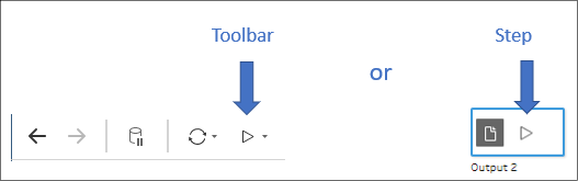
Figure 15.45: The toolbar allows you to run the flow for all outputs or a single output, while the button on the output step will run the flow only for that output

Your final flow will look something like this:

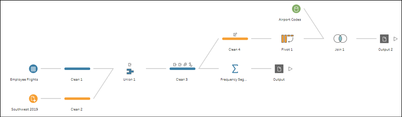
Figure 15.46: Your final flow will resemble this, but may be slightly different in appearance

The Chapter 15 Complete (clean).tfl file is a bit cleaned up with appropriate step labels and descriptions. As a good practice, try to rename your steps and include descriptions so that your flow is easier to understand. Here is how the cleaned version looks:

Figure 15.47: This flow is cleaned up and contains "self-documentation"

Once the flow has been executed, open the Airline Travel.twb workbook in the Learning TableauChapter 15 directory to see how the data might be used and to explore it on your own:

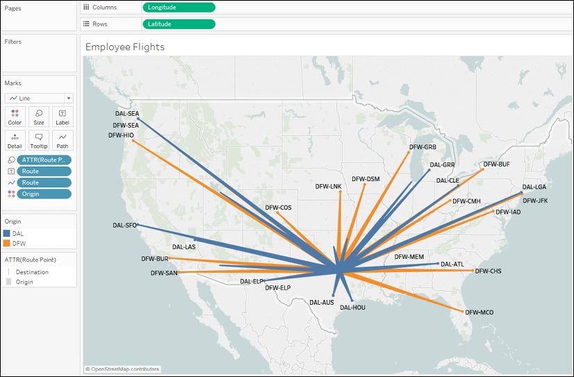
Figure 15.48: Exploring the data in the Airline Travel.twb workbook

With our example concluded, let's wrap up by considering some options for automating Tableau Prep flows.

Options for automating flows

Tableau Prep Builder allows you to design and run flows using the application. Sometimes, data cleansing and prepping will be a one-time operation to support an ad hoc analysis. However, you will often want to run a flow subsequently to capture new or changed data and to cleanse and shape it according to the same pattern. In these cases, you'll want to consider some options for automating the flow:

• Tableau Prep Builder may be run via a command line. You may supply JSON files to define credentials for input or output data connections. This enables you to use scripting and scheduling utilities to run the flow without manually opening and running the Tableau Prep interface. Details on this option are available from Tableau Help: https://onlinehelp.tableau.com/current/prep/en-us/prep_save_share.htm#refresh-output-files-from-the-command-line.
• Tableau Prep Conductor, an add-on to Tableau Server, gives you the ability to publish entire flows from Tableau Prep Builder to Tableau Server and then either run them on demand or on a custom schedule. It also provides monitoring and troubleshooting capabilities.

Summary

Tableau Prep's innovative paradigm of hands-on data cleansing and shaping with instant feedback greatly extends the Tableau platform and gives you incredible control over your data. In this chapter, we considered the overall interface and how it allows you to iteratively and rapidly build out a logical flow to clean and shape data for the desired analysis or visualization.

Through a detailed, yet practical, example that was woven throughout this chapter, we explored every major transformation in Tableau Prep, from inputs to unions, joins, aggregates and pivots, to outputs. Along the way, we also examined other transformations and capabilities, including calculations, splits, merges, and the grouping of values. This gives you a foundation for molding and shaping data in any way you need.

In the next chapter, we'll conclude with some final thoughts on how you can leverage Tableau's platform to share your analysis and data stories!