5

Leveraging Level of Detail Calculations

Having considered row-level and aggregate calculations, it's time to turn our attention to the third of the four main types of calculations: level of detail calculations.

Level of detail calculations (sometimes referred to as LOD calcs or LOD expressions) allow you to perform aggregations at a specified level of detail, which may be different from the level of detail that is defined in the view. You can leverage this capability to perform a wide variety of analyses that would otherwise be quite difficult.

In this chapter, we'll cover the following:

• Overview of level of detail
• Level of detail calculation syntax and variations
• Examples of FIXED level of detail calculations
• Examples of INCLUDE level of detail calculations
• Examples of EXCLUDE level of detail calculations

Overview of level of detail

What does the term level of detail mean? A lot depends on the context in which the term is used. Within Tableau, we'll distinguish several levels of detail, each of which is vitally important to understand in order to properly analyze data:

• Data level of detail: Sometimes referred to as the grain of the data, this is the level of detail defined by a single record of the data set. When you can articulate what one record of the data represents (for example, "Every record represents a single order" or "There is one record for every customer"), then you have a good understanding of the data level of detail. Row-level calculations operate at this level.
• View level of detail: We've previously discussed that the combination of fields used as dimensions in the view defines the view level of detail. Normally in a view, Tableau draws a single mark for each distinct combination of values present in the data for all the dimensions in the view. For example, if Customer and Year are the two dimensions in your view, Tableau will draw a mark (such as a bar or circle) for each Customer/Year combination present in the data (that is not excluded by a filter). Aggregate calculations operate at this level.
• Calculated level of detail: This is a separate level of detail defined by a calculation. As we'll see, you may use any number of dimensions to define the level of detail. Level of detail calculations are used to define this level.

Consider the following data set, with a data level of detail of one record per customer:

Customer	State	Membership Date	Membership Level	Orders
Neil	Kansas	2009-05-05	Silver	1
Jeane	Kansas	2012-03-17	Gold	5
George	Oklahoma	2016-02-01	Gold	10
Wilma	Texas	2018-09-17	Silver	4

In this case, each record defines a single unique customer. If we were to perform a row-level calculation, such as DATEDIFF('year', [Membership Date], TODAY()) to determine the number of years each customer has been a member, then the result would be calculated per record.

Now consider a view created from the data with a view level of detail of state:

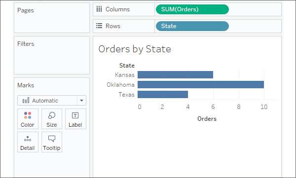
Figure 5.1: The view level of detail of state

As the only dimension in the view, State defines the view level of detail. There is one mark per state, and calculations and fields used as aggregates, such as SUM(Orders), will be performed per state.

Based on that particular view, we might want to enhance our understanding by asking additional questions, such as the following:

• Which customer was the first member of each state in the view?
• How does the number of orders per state compare to the average number of orders for all states?
• Which membership level had the highest or lowest number of orders per state?

In each case, the question involves a level of detail that is different from the view (the minimum membership date per state compared to each individual customer, the average orders overall compared to orders per state, and the minimum or maximum number of orders per membership level per state). In some cases, it might make sense to build a new view to answer these questions. But sometimes we want to supplement an existing view or compare different levels of detail in the same view. Level of detail calculations provide a solution!

Level of detail calculations

Before getting into practical examples of using level of detail calculations, let's take a moment to understand the syntax and types of level of detail calculations.

Level of detail syntax

Level of detail calculations follow this basic pattern of syntax:

{FIXED|INCLUDE|EXCLUDE [Dim 1],[Dim 2] : AGG([Field])}

The definitions of the preceding declaration are as follows:

• FIXED, INCLUDE, and EXCLUDE are keywords that indicate the type of level of detail calculation. We'll consider the differences in detail in the following section.
• Dim 1, Dim 2 (and as many dimensions that are needed) is a comma-separated list of dimension fields that defines the level of detail at which the calculation will be performed.
• AGG is the aggregate function you wish to perform (such as SUM, AVG, MIN, and MAX).
• Field is the value that will be aggregated as specified by the aggregation you choose.

Level of detail types

Three types of level of detail calculations are used in Tableau: FIXED, INCLUDE, and EXCLUDE.

FIXED

Fixed level of detail expressions work at the level of detail that's specified by the list of dimensions in the code, regardless of what dimensions are in the view. For example, the following code returns the average orders per state, regardless of what other dimensions are in the view:

{FIXED [State] : AVG([Orders])} 

You may include as many dimensions as needed or none at all. The following code represents a fixed calculation of the average orders for the entire set of data from the data source:

{FIXED : AVG([Orders])} 

Alternately, you might write the calculation in the following way with identical results:

{AVG([Orders])}

INCLUDE

Include level of detail expressions aggregate at the level of detail that's determined by the dimensions in the view, along with the dimensions listed in the code. For example, the following code calculates the average orders at the level of detail that's defined by dimensions in the view, but includes the dimension Membership Level, even if Membership Level is not in the view:

{INCLUDE [Membership Level] : AVG([Orders])} 

EXCLUDE

Exclude level of detail expressions aggregate at the level of detail determined by the dimensions in the view, excluding any listed in the code. For example, the following code calculates the average number of orders at the level of detail defined in the view, but does not include the Customer dimension as part of the level of detail, even if Customer is in the view:

{EXCLUDE [Customer] : AVG([Orders])}

An illustration of the difference level of detail can make

As you analyze data, one thing you might often wonder is how slices of data relate to the overall picture. For example, you might wonder how the number of orders for each state in the view above relates to the overall average number of orders. One quick and easy option is to add an Average Line to the view from the Analytics tab, by dragging and dropping like this:

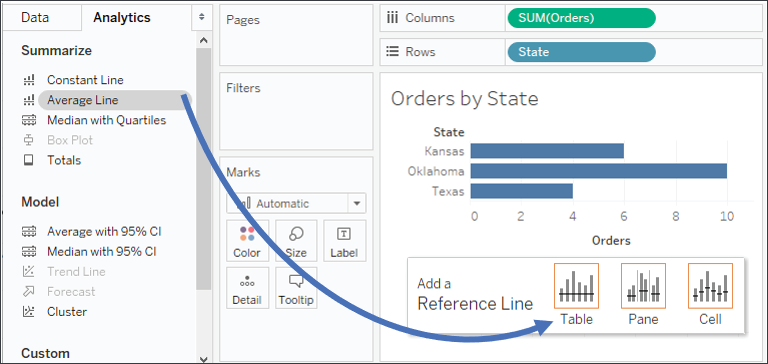
Figure 5.2: Adding an average line to the view

You'll end up with an average line that looks like this:

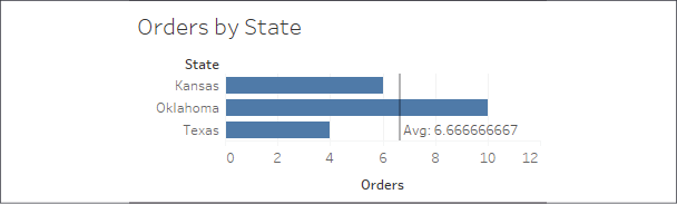
Figure 5.3: The overall average is reported as 6.66667. This is the average per state

But is 6.66667 truly the average number of orders overall? It turns out that it's not. It's actually the average of the sum of the number of orders for each state: (6 + 10 + 4) / 3. Many times, that average line (that is, the average of the total number of orders per state) is exactly what we want to compare when using aggregate numbers.

But sometimes, we might want to calculate the true overall average. To get the average number of orders present in the entire data set, we might consider creating a calculation named Overall Average Number of Orders and using a fixed level of detail calculation like this:

{FIXED : AVG([Orders])} 

Adding that calculated field to the Detail part of the Marks card and editing the reference line to use that field instead gives us a different result:

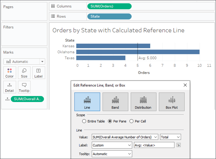
Figure 5.4: The true overall average number of orders per customer is 5

You'll recall that the original data set had four records, and a quick check validates the result:

(1 + 5 + 10 + 4) / 4 = 5

Now we have examined how level of detail calculations make a real difference; let's look at some practical examples.

Examples of fixed level of detail calculations

As we turn our attention to some practical examples of level of detail calculations, we'll use the Chapter 05 Loans data set contained in the Chapter 05 workbook. The true data set contains many more records, but here is an example of the kinds of data it contains:

Date	Portfolio	Loan Type	Balance	Open Date	Member Name	Credit Score	Age	State
3/1/2020	Auto	New Auto	15987	9/29/2018	Samuel	678	37	California
7/1/2020	Mortgage	1st Mortgage	96364	8/7/2013	Lloyd	768	62	Ohio
3/1/2020	Mortgage	HELOC	15123	4/2/2013	Inez	751	66	Illinois
3/1/2020	Mortgage	1st Mortgage	418635	9/30/2015	Patrick	766	60	Ohio
5/1/2020	Auto	Used Auto	1151	10/22/2018	Eric	660	44	Pennsylvania
…	…	…	…	…	…	…	…	…
…	…	…	…	…	…	…	…	…

The data set represents historical data for loans for members at a bank, credit union, or similar financial institution. Each record is a monthly snapshot of a loan and contains the date of the snapshot along with fields that describe the loan (Portfolio, Loan Type, Balance, and Open Date) and fields for the member (Name, Credit Score, Age, and State).

As in previous chapters, the goal is to understand key concepts and some key patterns. The following are only a few examples of all the possibilities presented by level of detail calculations.

Was a member ever at risk?

Let's say branch management has determined that any member who has ever had a credit score of less than 550 is considered to be at risk and eligible for special assistance. Consider the history for the following three individuals:

Figure 5.5: Credit scores for three individuals with scores under the 550 threshold indicated via arrows

Every month, a new snapshot of history is recorded. Loan balances often change along with the member's credit score. Some members have never been at risk. The first member, Vicki, has 699 as her lowest recorded score and has never been at risk. However, both Charles and Thomas had periods in the history where their credit scores fell below the threshold (indicated with arrows in the preceding screenshot).

A simple row-level calculation, such as [Credit Score] < 550, could identify each record where the monthly snapshot of credit score indicated a risk. But members whose scores fluctuated below and above the threshold would have records that were alternately TRUE or FALSE.

We want every record for a given member to be TRUE if any of the records for that member are below the threshold and FALSE if none of the records are below the threshold.

One solution is to use a level of detail calculation, which we'll name Member Ever at Risk?, with the code:

{FIXED [Member ID] : MIN([Credit Score])} < 550

This calculation determines the lowest credit score for each member and compares it to the risk threshold of 550. The result is the same for each record for a given member, as you can see here:

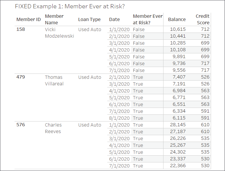
Figure 5.6: The Member Ever at Risk? field is True or False for all records of a given member

Notice that every record contains the result for the relevant member. This illustrates one key concept for fixed level of detail calculations: while the calculation is an aggregation at a defined level of detail, the results are at the row level. That is, the TRUE or FALSE value is calculated at the member level, but the results are available as row-level values for every record for that member.

This enables all kinds of analysis possibilities, such as:

• Filtering to include only at-risk members but retaining all records for their history. If you instead filtered based on individual credit score, you'd lose all records for parts of the history where the credit score was above the threshold. Those records might be critical for your analysis.
• Correctly counting members as either at risk or not while avoiding counting them for both cases if the history fluctuated.
• Comparing members who were or were not at risk at other levels of detail. For example, this view shows the number of members who were at risk or not at risk by portfolio:

  

  Figure 5.7: We can implement some brushing to show what proportion of members has ever been at risk

This is a single example of the kinds of analysis made simple with level of detail calculations. There's so much more we can do and we'll see another example next!

Latest balance for a member

Many data sets contain a series of events or a history of transactions. You may find yourself asking questions such as:

• What diagnoses are common for a patient's first visit to the hospital?
• What was the last reported status of each computer on the network?
• How much did each customer spend on their last order?
• How much did the first trade of the week make compared to the last?

None of these questions is simply asking when the earliest or latest event happened. A simple MIN or MAX aggregation of the date would provide that answer. But with these questions, there is the added complexity of asking for additional detail about what happened on the earliest or latest dates. For these kinds of questions, level of detail calculations provide a way to arrive at answers.

Consider the following three members' data contained in the Chapter 05 Loans data set:

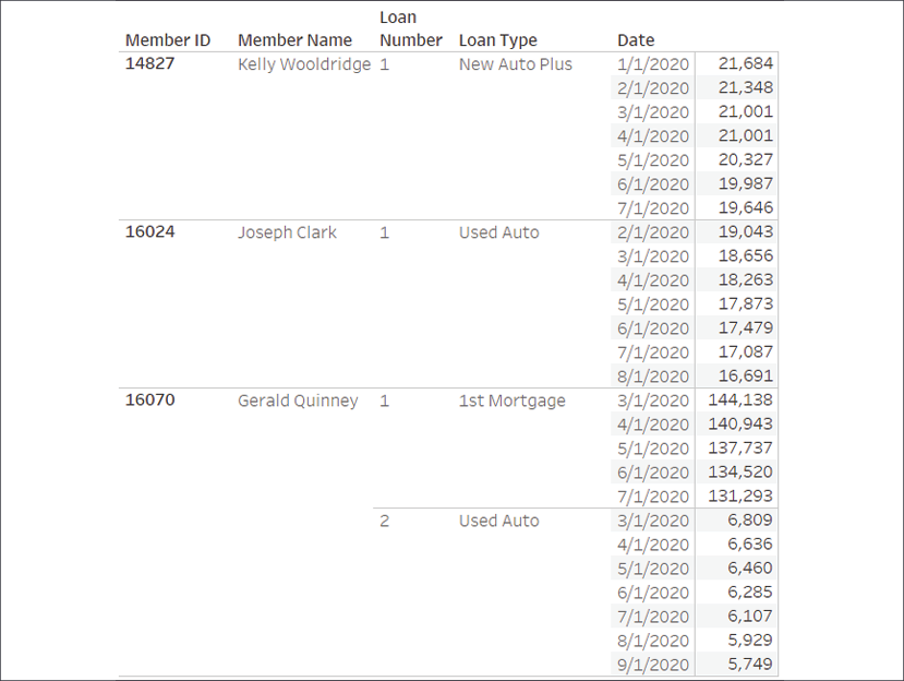
Figure 5.8: The data for three selected members in the Loans data set

Each has a history of balances for each of their loans. However, the most recent date of history differs for each loan. Kelly's most recent balance is given for July. Joseph's latest balance is for August. Gerald has two loans: the first has the most recent balance for July and the second has the most recent balance for September.

What if you want to identify only the records that represent the latest known balance for a member? You might consider using a fixed level of detail calculation called Latest Date per Member/Loan with code such as this:

{FIXED [Member ID],[Loan Number] : MAX([Date])} = [Date]

This determines the maximum date per member per loan and compares the result to each row-level date, returning TRUE for matches and FALSE otherwise.

You can see the results of the calculation here:

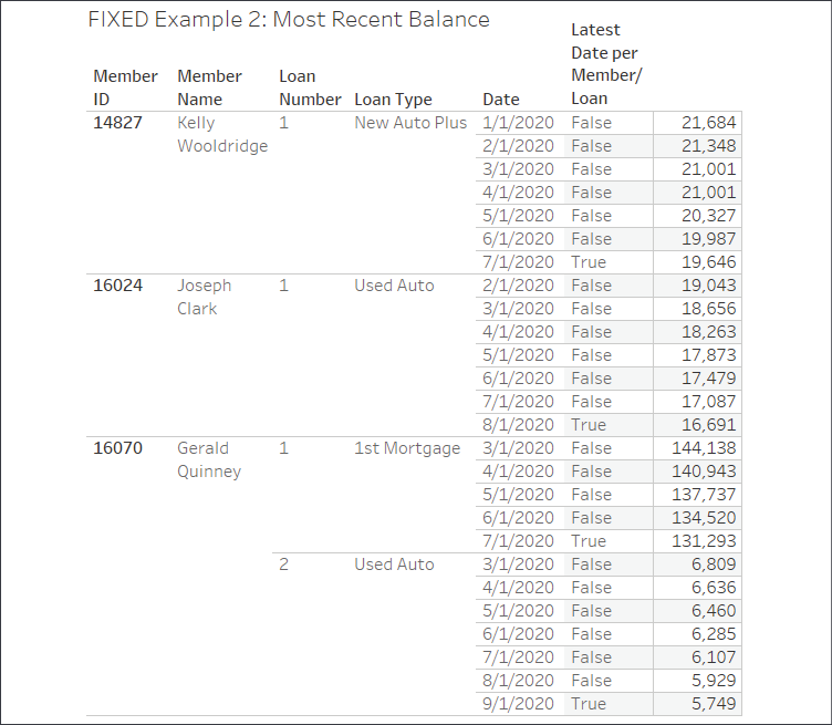
Figure 5.9: The latest date per loan per person is indicated by a True value for the calculation

If you had wanted to determine the first record for each loan, you would have simply changed MAX to MIN in the code. You can use the level of detail calculation's row-level TRUE / FALSE result as a filter to keep only the latest records, or even as part of other calculations to accomplish an analysis, such as comparing, starting, and ending balances.

We've just seen how fixed level of detail calculations can be leveraged to answer some complex questions. Let's continue by examining include level of detail expressions.

Example of include level of detail expressions

Include level of detail calculations can be very useful when you need to perform certain calculations at levels of detail that are lower (more detailed) than the view level of detail. Let's take a look at an example.

Average loans per member

Some members have a single loan. Some have two or three or possibly more. What if we wanted to see how many loans the average member has on a state by state basis? Let's consider how we might go about that.

We'll start with a sheet where the view level of detail is State:

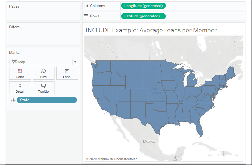
Figure 5.10: The starting place for the example—a filled map by state

It would be relatively easy to visualize the average credit score or average balance per state. But what if we want to visualize the average number of loans per member for each state? While there are several possible approaches to solving this kind of problem, here we'll consider using the following level of detail expression named Number of Loans per Member:

{INCLUDE [Member ID] : COUNTD([Loan Number])}

This code returns a distinct count of loan numbers at a level of detail that includes the member ID along with all dimensions that defined the view level of detail (state, in this case). When we add the calculation to the view, we'll need to decide how to aggregate it. In this case, we want the average number of loans per member, so we'll select Measure | Average from the dropdown on the field, revealing an interesting geographic pattern:

Figure 5.11: Using the Include level of detail calculation to create a gradient of color to show average loans per member

As you think through how include level of detail calculations work, you might want to construct a crosstab at the level of detail:

Figure 5.12: A crosstab helps illustrate how the distinct count of loans can be used as a basis for an average

State, the first dimension on Rows, comes from the view level of detail. Member ID has been included in the crosstab to simulate the dimension included in the level of detail expression. COUNTD(Loan Number) gives the number of loans per member. Averaging the values for all the members in the state gives the state average. A quick check for North Dakota gives us an average of 1.2 loans per member, which matches the map visualization exactly.

In this case, the include level of detail expression gives us a useful solution. There are some alternative ways to solve and it is helpful to consider some of these as you think through how you might solve similar issues. We'll consider those next.

Alternative approaches

It's worth noting that the above dataset actually allows you to use MAX([Loan Number]) instead of COUNTD([Loan Number]) as the number simply increments for each member based on how many loans they have. The highest number is identical to the number of loans for that member. In a significantly large data set, the MAX calculation should perform better.

There are also a few other approaches to solving this problem, such as the calculation. For example, you could write the following code:

COUNTD(STR([Member ID]) + "_" + STR([Loan Number])) 
/ 
COUNTD([Member ID])

This code takes the distinct count of loans and divides it by the distinct count of members. In order to count the distinct number of loans, the code creates a unique key by concatenating a string of a member ID and a loan number.

Another approach would be to use a fixed level of detail expression, such as:

{FIXED [State],[Member ID] : COUNTD([Loan Number])}

This calculation results in the same level of detail as the include expression and uses the same distinct count of loan number. It turns out that in this data set, each member belongs to only a single state, so state wouldn't necessarily have to be included in the fixed level of detail expression. However, if you wanted to change the level of detail you'd need to adjust the calculation, whereas, with the include expression, you'd only have to add or remove dimensions to the view.

With the include example along with some alternatives in mind, let's turn our attention to an example of exclude level of detail calculations.

Example of exclude level of detail calculations

Exclude level of detail calculations are useful when you want to perform certain calculations at higher (less detailed) levels than the view level of detail. The following example will demonstrate how we can leverage this functionality.

Average credit score per loan type

In this example, we'll answer the following question: how does the average credit score for a given loan type compare to the overall average for the entire portfolio?

Take the following view, which shows the average credit score per loan type (where loan types are grouped into portfolios):

Figure 5.13: This crosstab shows the average credit score per loan type

What if we wanted to compare the average credit score of each loan type with the overall average credit score for the entire portfolio? We could accomplish this with an exclude level of detail calculation that looks like this:

{EXCLUDE [Loan Type] : AVG([Credit Score])}

This removes Loan Type from the level of detail and the average is calculated only per portfolio. This gives us results like the following:

Figure 5.14: The exclude level of detail expression removes Loan Type so the average is only at the portfolio level

You'll notice that the same value for the average excluding loan type is repeated for each loan type. This is expected because the overall average is at the portfolio level and is not affected by the loan type. As is, this is perhaps not the most useful view. But we can extend the calculation a bit to give us the difference between the overall portfolio average and the average of each loan type. The code would look like this:

AVG([Credit Score]) - AVG([Average Credit Score Excluding Loan Type])

This takes the average at the view level of detail (loan type and portfolio) and subtracts the average at the portfolio level to give us the difference between each loan type average and the overall portfolio average. We might rearrange the view to see the results visually, like this:

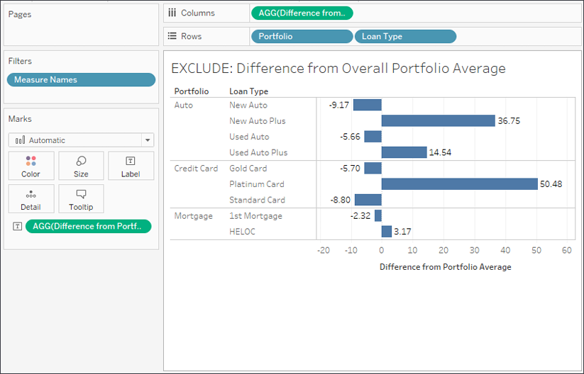
Figure 5.15: The final view shows the difference between the loan type average credit score and the overall portfolio average

Exclude level of detail expressions give us the ability to analyze differences between the view level of detail and higher levels of detail.

Summary

Level of detail expressions greatly extend what you can accomplish with calculations. You now have a toolset for working with data at different levels of detail. With fixed level of detail calculations, you can identify the first or last event in a series or whether a condition is ever true across entire subsets of data. With include expressions, you can work at lower levels of detail and then summarize those results in a view. With exclude expressions, you can work at higher levels of detail, greatly expanding analysis possibilities.

In the next chapter, we'll explore the final main type of calculations: table calculations. These are some of the most powerful calculations in terms of their ability to solve problems, and they open up incredible possibilities for in-depth analysis. In practice, they range from very easy to exceptionally complex.