2
Connecting to Data in Tableau
Tableau offers the ability to connect to nearly any data source. It does this with a unique paradigm that leverages the power and efficiency of existing database engines or alternately extracts the data locally. We'll look at joins, blends, unions, and the brand new object model in Chapter 13, Understanding the Tableau Data Model, Joins, and Blends. In this chapter, we'll focus on essential concepts of how Tableau connects to and works with data. We'll cover the following topics:
- The Tableau paradigm
- Connecting to data
- Managing data source metadata
- Working with extracts instead of live connections
- Filtering data
We'll start by gaining an understanding of the underlying paradigm of how Tableau works with data.
The Tableau paradigm
The unique and exciting experience of working with data in Tableau is a result of VizQL (Visual Query Language).
VizQL was developed as a Stanford University research project, focusing on the natural ways that humans visually perceive the world and how that could be applied to data visualization. We naturally perceive differences in size, shape, spatial location, and color. VizQL allows Tableau to translate your actions, as you drag and drop fields of data in a visual environment, into a query language that defines how the data encodes those visual elements. You will never need to read, write, or debug VizQL. As you drag and drop fields onto various shelves defining size, color, shape, and spatial location, Tableau will generate the VizQL behind the scenes. This allows you to focus on visualizing data, not writing code!
One of the benefits of VizQL is that it provides a common way of describing how the arrangement of various fields in a view defines a query related to the data. This common baseline can then be translated into numerous flavors of SQL, MDX, and Tableau Query Language (TQL, used for extracted data). Tableau will automatically perform the translation of VizQL into a native query to be run by the source data engine.
In its simplest form, the Tableau paradigm of working with data looks like the following diagram:
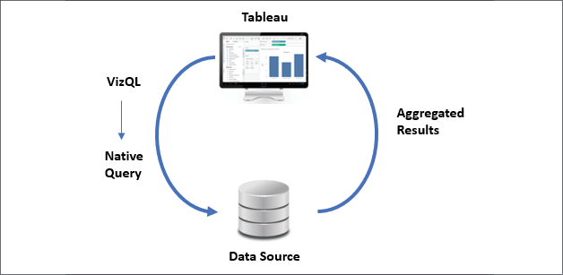
Figure 2.1: The basic Tableau paradigm for working with data
Let's look at how this paradigm works in a practical example.
A simple example
Open the Chapter 02 Starter.twbx workbook located in the Learning TableauChapter 02 directory and navigate to the Tableau Paradigm sheet. That view was created by dropping the Region dimension on Columns and the Sales measure on Rows. Here is a screenshot:
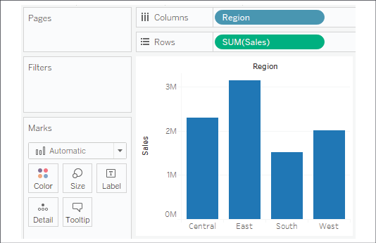
Figure 2.2: This bar chart is the result of a query that returned four aggregate rows of data
The view is defined by two fields. Region is the only dimension, which means it defines the level of detail in the view and slices the measure so that there will be a bar per region. Sales is used as a measure aggregated by summing each sale within each region. (Notice also that Region is discrete, resulting in column headers while Sales is continuous, resulting in an axis.)
For the purpose of this example (although the principle is applicable to any data source), let's say you were connected live to a SQL Server database with the Superstore data stored in a table. When you first create the preceding screenshot, Tableau generates a VizQL script, which is translated into an SQL script and sent to the SQL Server. The SQL Server database engine evaluates the query and returns aggregated results to Tableau, which are then rendered visually.
The entire process would look something like the following diagram in Tableau's paradigm:
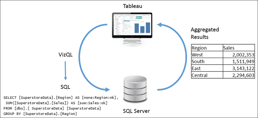
Figure 2.3: Tableau generated the bar chart in the previous image using a paradigm like this
There may have been hundreds, thousands, or even millions of rows of sales data in SQL Server. However, when SQL Server processes the query, it returns aggregate results. In this case, SQL Server returns only four aggregate rows of data to Tableau—one row for each region.
On occasion, a database administrator may want to find out what scripts are running against a certain database to debug performance issues or to determine more efficient indexing or data structures. Many databases supply profiling utilities or log execution of queries. In addition, you can find SQL or MDX generated by Tableau in the logs located in the My Tableau RepositoryLogs directory.
You may also use Tableau's built-in Performance Recorder to locate the queries that have been executed. From the top menu, select Help | Settings and Performance | Start Performance Recording, then interact with a view, and finally, stop the recording from the menu. Tableau will open a dashboard that will allow you to see tasks, performance, and queries that were executed during the recording session.
To see the aggregate data that Tableau used to draw the view, press Ctrl + A to select all the bars, and then right-click one of them and select View Data.

Figure 2.4: Use the View Data tooltip option to see a summary or underlying data for a mark
This will reveal a View Data window:
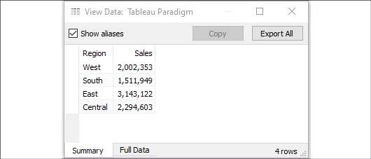
Figure 2.5: The Summary tab displays the aggregate data Tableau used to render each mark in the view
The View Data screen allows you to observe the data in the view. The Summary tab displays the aggregate-level data that was used to render the view. The Sales values here are the sum of sales for each region. When you click the Full Data (previously named Underlying) tab, Tableau will query the data source to retrieve all the records that make up the aggregate records. In this case, there are 9,426 underlying records, as indicated on the status bar in the lower-right corner of the following screenshot:

Figure 2.6: The Full Data tab reveals the row-level data in the database
Tableau did not need 9,426 records to draw the view and did not request them from the data source until the Full Data data tab was clicked.
Database engines are optimized to perform aggregations on data. Typically, these database engines are also located on powerful servers. Tableau leverages the optimization and power of the underlying data source. In this way, Tableau can visualize massive datasets with relatively little local processing of the data.
Additionally, Tableau will only query the data source when you make changes requiring a new query or a view refresh. Otherwise, it will use the aggregate results stored in a local cache, as illustrated here:

Figure 2.7: The first rendering with a given set of fields queries the data source directly. Subsequent renderings will query the cache, even if the same fields are re-arranged in the view
In the preceding example, the query with Region as a dimension and the sum of Sales as a measure will only be issued once to the data source. When the four rows of aggregated results are returned, they are stored in the cache. After the initial rendering, if you were to move Region to another visual encoding shelf, such as color, or Sales to a different visual encoding shelf, such as size, then Tableau will retrieve the aggregated rows from the cache and simply re-render the view.
You can force Tableau to bypass the cache and refresh the data from a data source by pressing F5 or selecting your data source from the Data menu and selecting Refresh. Do this any time you want a view to reflect the most recent changes in a live data source.
If you were to introduce new fields into the view that did not have cached results, Tableau would send a new query to the data source, retrieve the aggregated results, and add those results to the cache.
Connecting to data
There is virtually no limit to the data that Tableau can visualize! Almost every new version of Tableau adds new native connectors. Tableau continues to add native connectors for cloud-based data. The web data connector allows you to write a connector for any online data you wish to retrieve. The Tableau Hyper API allows you to programmatically read and write extracts of data, enabling you to access data from any source and write it to a native Tableau format. Additionally, for any database without a built-in connection, Tableau gives you the ability to use a generic ODBC connection.
You may have multiple data sources in the same workbook. Each source will show up under the Data tab on the left sidebar.
Although the terms are often used interchangeably, it is helpful to make a distinction. A connection technically refers to the connection made to data in a single location, such as tables in a single database, or files of the same type in the same directory structure. A data source may contain more than one connection that can be joined together, such as a table in SQL Server joined to tables in a Snowflake database that are joined to an Excel table. You can think about it this way: a Tableau workbook may contain one or more data sources and each data source may contain one or more connections. We'll maintain this distinction throughout the book.
This section will focus on a few practical examples of connecting to various data sources. There's no way to cover every possible type of connection but we will cover several that are representative of others. You may or may not have access to some of the data sources in the following examples. Don't worry if you aren't able to follow each example. Merely observe the differences.
Connecting to data in a file
File-based data includes all sources of data where the data is stored in a file. File-based data sources include the following:
- Extracts: A
.hyperor.tdefile containing data that was extracted from an original source. - Microsoft Access: An
.mdbor.accdbdatabase file created in Access. - Microsoft Excel: An
.xls,.xlsx, or.xlsmspreadsheet created in Excel. Multiple Excel sheets or sub-tables may be joined or unioned together in a single connection. - Text file: A delimited text file, most commonly
.txt,.csv, or.tab. Multiple text files in a single directory may be joined or unioned together in a single connection. - Local cube file: A
.cubfile that contains multi-dimensional data. These files are typically exported from OLAP databases. - Adobe PDF: A
.pdffile that may contain tables of data that can be parsed by Tableau. - Spatial file: A wide variety of spatial formats are supported such as
.kml,.shp,.tab,.mif, spatial JSON, and ESRI database files. These formats contain spatial objects that can be rendered by Tableau. - Statistical file: A
.sav,.sas7bdat,.rda, or.rdatafile generated by statistical tools, such as SAS or R. - JSON file: A
.jsonfile that contains data in JSON format.
In addition to those mentioned previously, you can connect to Tableau files to import connections that you have saved in another Tableau workbook (.twb or .twbx). The connection will be imported, and changes will only affect the current workbook.
Follow this example to see a connection to an Excel file:
- Navigate to the Connect to Excel sheet in the
Chapter 02 Starter.twbxworkbook. - From the menu, select Data | New Data Source and select Microsoft Excel from the list of possible connections.
- In the open dialogue, open the
Superstore.xlsxfile from theLearning TableauChapter 02directory. Tableau will open the Data Source screen. You should see the two sheets of the Excel document listed on the left. - Double-click the Orders sheet and then the Returns sheet. Tableau will prompt you with an Edit Relationship dialog. We'll cover relationships in depth in Chapter 13, Understanding the Tableau Data Model, Joins, and Blends. For now, accept the defaults by closing the dialog.
Your data source screen should look similar to the following screenshot:
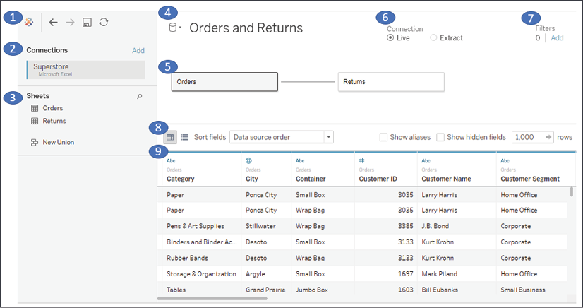
Figure 2.8: The data source screen with two objects (Orders and Returns)
Take some time to familiarize yourself with the Data Source screen interface, which has the following features (numbered in the preceding screenshot):
- Toolbar: The toolbar has a few of the familiar controls, including undo, redo, and save. It also includes the option to refresh the current data source.
- Connections: All the connections in the current data source. Click Add to add a new connection to the current data source. This allows you to join data across different connection types. Each connection will be color-coded so that you can distinguish what data is coming from which connection.
- Sheets (or Tables): This lists all the tables of data available for a given connection. This includes sheets, sub-tables, and named ranges for Excel; tables, views, and stored procedures for relational databases; and other connection-dependent options, such as New Union or Custom SQL.
- Data Source Name: This is the name of the currently selected data source. You may select a different data source using the drop-down arrow next to the database icon. You may click the name of the data source to edit it.
- Object / Data Model Canvas: Drop sheets and tables from the left into this area to make them part of the connection. You may add additional tables by dragging and dropping or double-clicking them. Each will be added as an object to the object model. You may also add tables as unions or double-click an object to edit the underlying tables and joins. We'll cover the details extensively in Chapter 13, Understanding the Tableau Data Model, Joins, and Blends. For now, simply note that Orders and Returns are related together by the Order ID.
- Live or Extract Options: For many data sources, you may choose whether you would like to have a live connection or an extracted connection. We'll look at these in further detail later in the chapter.
- Data Source Filters: You may add filters to the data source. These will be applied at the data-source level, and thus to all views of the data using this data source in the workbook.
- Preview Pane Options: These options allow you to specify whether you'd like to see a preview of the data or a list of metadata, and how you would like to preview the data (examples include alias values, hidden fields shown, and how many rows you'd like to preview).
- Preview Pane/Metadata View: Depending on your selection in the options, this space either displays a preview of data or a list of all fields with additional metadata. Notice that these views give you a wide array of options, such as changing data types, hiding or renaming fields, and applying various data transformation functions. We'll consider some of these options in this and later chapters.
Once you have created and configured your data source, you may click any sheet to start using it.
Conclude this exercise with the following steps:
- Click the data source name to edit the text and rename the data source to
Orders and Returns.
- Navigate to the Connect to Excel sheet and, using the
Orders and Returnsdata source, create a time series showing Returns (Count) by Return Reason. Your view should look like the following screenshot:
Figure 2.9: The number of returns by return reason
If you need to edit the connection at any time, select Data from the menu, locate your connection, and then select Edit Data Source.... Alternately, you may right-click any data source under the Data tab on the left sidebar and select Edit Data Source..., or click the Data Source tab in the lower-left corner. You may access the data source screen at any time by clicking the Data Source tab in the lower-left corner of Tableau Desktop.
Connecting to data on a server
Database servers, such as SQL Server, Snowflake, Vertica, and Oracle, host data on one or more server machines and use powerful database engines to store, aggregate, sort, and serve data based on queries from client applications. Tableau can leverage the capabilities of these servers to retrieve data for visualization and analysis. Alternately, data can be extracted from these sources and stored in an extract.
As an example of connecting to a server data source, we'll demonstrate connecting to SQL Server. If you have access to a server-based data source, you may wish to create a new data source and explore the details. However, this specific example is not included in the workbook in this chapter.
As soon as the Microsoft SQL Server connection is selected, the interface displays options for some initial configuration as follows:
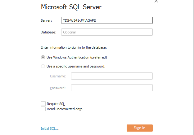
Figure 2.10: The connection editor for Microsoft SQL Server
A connection to SQL Server requires the Server name, as well as authentication information.
A database administrator can configure SQL Server to Use Windows Authentication or a SQL Server username and password. With SQL Server, you can also optionally allow reading uncommitted data. This can potentially improve performance but may also lead to unpredictable results if data is being inserted, updated, or deleted at the same time as Tableau is querying. Additionally, you may specify SQL to be run at connect time using the Initial SQL... link in the lower-left corner.
In order to maintain high standards of security, Tableau will not save a password as part of a data source connection. This means that if you share a workbook using a live connection with someone else, they will need to have credentials to access the data. This also means that when you first open the workbook, you will need to re-enter your password for any connections requiring a password.
Once you click the orange Sign In button, you will see a screen that is very similar to the connection screen you saw for Excel. The main difference is on the left, where you have an option for selecting a Database, as shown in the following screenshot:

Figure 2.11: Once connected to a database, Tableau will display tables, views, and stored procedures as options to add to the object model
Once you've selected a database, you will see the following:
- Table: This shows any data tables or views contained in the selected database.
- New Custom SQL: You may write your own custom SQL scripts and add them as tables. You may join these as you would any other table or view.
- New Union: You may union together tables in the database. Tableau will match fields based on name and data type, and you may additionally merge fields as needed.
- Stored Procedures: You may use a stored procedure that returns a table of data. You will be given the option of setting values for stored procedure parameters or using or creating a Tableau parameter to pass values.
Once you have finished configuring the connection, click a tab for any sheet to begin visualizing the data.
Using extracts
Any data source that is using an extract will have a distinctive icon that indicates the data has been pulled from an original source into an extract, as shown in the following screenshot:

Figure 2.12: The icon next to a data source indicates whether it is extracted or not
The first data connection in the preceding data pane is extracted, while the second is not. After an extract has been created, you may choose to use the extract or not. When you right-click a data source (or Data from the menu and then the data source), you will see the following menu options:

Figure 2.13: The context menu for a data connection in the Data pane with Extract options numbered
Let's cover them in more detail:
- Refresh: The Refresh option under the data source simply tells Tableau to refresh the local cache of data. With a live data source, this would re-query the underlying data. With an extracted source, the cache is cleared and the extract is required, but this Refresh option does not update the extract from the original source. To do that, use Refresh under the Extract sub-menu (see number 4 in this list).
- Extract Data...: This creates a new extract from the data source (replacing an existing extract if it exists).
- Use Extract: This option is enabled if there is an extract for a given data source. Unchecking the option will tell Tableau to use a live connection instead of the extract. The extract will not be removed and may be used again by checking this option at any time. If the original data source is not available to this workbook, Tableau will ask where to find it.
- Refresh: This Refresh option refreshes the extract with data from the original source. It does not optimize the extract for some changes you make (such as hiding fields or creating new calculations).
- Append Data from File... or Append Data from Data Source…:These options allow you to append additional files or data sources to an existing extract, provided they have the same exact data structure as the original source. This adds rows to your existing extract; it will not add new columns.
- Compute Calculations Now: This will restructure the extract, based on changes you've made since originally creating the extract, to make it as efficient as possible. Certain calculated fields may be materialized (that is, calculated once so that the resulting value can be stored) and newly hidden columns or deleted calculations will be removed from the extract.
- Remove: This removes the definition of the extract, optionally deletes the extract file, and resumes a live connection to the original data source.
- History: This allows you to view the history of the extract and refreshes.
- Properties: This enables you to view the properties of the extract, such as the location, underlying source, filters, and row limits.
Let's next consider the performance ramifications of using extracts.
Connecting to data in the cloud
Certain data connections are made to data that is hosted in the cloud. These include Amazon RDS, Google BigQuery, Microsoft SQL Azure, Snowflake, Salesforce, Google Sheets, and many others. It is beyond the scope of this book to cover each connection in depth, but as an example of a cloud data source, we'll consider connecting to Google Sheets.
Google Sheets allows users to create and maintain spreadsheets of data online. Sheets may be shared and collaborated on by many different users. Here, we'll walk through an example of connecting to a sheet that is shared via a link.
To follow the example, you'll need a free Google account. With your credentials, follow these steps:
- Click the Add new data source button on the toolbar, as shown here:

Figure 2.14: The Add Data button
- Select Google Sheets from the list of possible data sources. You may use the search box to quickly narrow the list.
- On the next screen, sign in to your Google account and allow Tableau Desktop the appropriate permissions. You will then be presented with a list of all your Google Sheets, along with preview and search capabilities, as shown in the following screenshot:
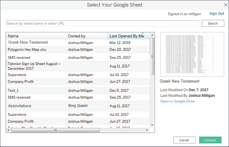
Figure 2.15: You may select any Google Sheet you have permissions to view or you may enter the URL for a shared sheet
- Enter the following URL (for convenience, it is included in the
Chapter 02 Starterworkbook in the Connect to Google Sheets tab, and may be copied and pasted) into the search box and click the Search button: https://docs.google.com/spreadsheets/d/1fWMGkPt0o7sdbW50tG4QLSZDwkjNO9X0mCkw-LKYu1A/edit?usp=sharing: - Select the resulting
Superstoresheet in the list and then click the Connect button. You should now see the Data Source screen. - Click the Data Source name to rename it to
Superstore (Google Sheets):
Figure 2.16: Renaming a Data Source
- For the purpose of this example, switch the connection option from Live to Extract. When connecting to your own Google Sheets data, you may choose either Live or Extract:

Figure 2.17: Switch between Live and Extract, Edit extract options, and Add Filters
- Click the tab for the Connect to Google Sheets sheet. You will be prompted for a location to save the extract. Accept the default name and save it in the
Learning TableauChapter 02directory (selecting Yes to overwrite the existing file if needed). The data should be extracted within a few seconds.
- Create a filled map of Profit by State, with Profit defining the Color and Label:

Figure 2.18: The filled map demonstrates the ability to connect to a cloud-based data source
If your location is outside the United States, you may need to change your regional settings for Tableau to properly show the states in the map. Use the menu and select File | Workbook Locale | More and select English (United States).
Now that we've seen a few specific examples of connecting to data, let's consider some shortcuts and how to manage our data sources.
Shortcuts for connecting to data
You can make certain connections very quickly. These options will allow you to begin analyzing more quickly:
- Paste data from the clipboard. If you have copied data in your system's clipboard from any source (for example, a spreadsheet, a table on a web page, or a text file), you can then paste the data directly into Tableau. This can be done using Ctrl + V, or Data | Paste Data from the menu. The data will be stored as a file and you will be alerted to its location when you save the workbook.
- Select File | Open from the menu. This will allow you to open any data file that Tableau supports, such as text files, Excel files, Access files (not available on macOS), spatial files, statistical files, JSON, and even offline cube (
.cub) files. - Drag and drop a file from Windows Explorer or Finder onto the Tableau workspace. Any valid file-based data source can be dropped onto the Tableau workspace or even the Tableau shortcut on your desktop or taskbar.
- Duplicate an existing data source. You can duplicate an existing data source by right-clicking and selecting Duplicate.
These shortcuts provide a quick way for analyzing the data you need. Let's turn our attention to managing the data sources.
Managing data source metadata
Data sources in Tableau store information about the connection(s). In addition to the connection itself (for example, database server name, database, and/or filenames), the data source also contains information about all the fields available (such as field name, data type, default format, comments, and aliases). Often, this data about the data is referred to as metadata.
Right-clicking a field in the data pane reveals a menu of metadata options. Some of these options will be demonstrated in a later exercise; others will be explained throughout the book. These are some of the options available via right-clicking:
- Renaming the field
- Hiding the field
- Changing aliases for values of a non-date dimension
- Creating calculated fields, groups, sets, bins, or parameters
- Splitting the field
- Changing the default use of a date or numeric field to either discrete or continuous
- Redefining the field as a dimension or a measure
- Changing the data type of the field
- Assigning a geographic role to the field
- Changing defaults for how a field is displayed in a visualization, such as the default colors and shapes, number or date format, sort order (for dimensions), or type of aggregation (for measures)
- Adding a default comment for a field (which will be shown as a tooltip when hovering over a field in the data pane, or shown as part of the description when Describe... is selected from the menu)
- Adding or removing the field from a hierarchy
Metadata options that relate to the visual display of the field, such as default sort order or default number format, define the overall default for a field. However, you can override the defaults in any individual view by right-clicking the active field on the shelf and selecting the desired options.
To see how this works, use the filled map view of Profit by State that you created in the Connect to Google Sheets view. If you did not create this view, you may use the Orders and Returns data source, though the resulting view will be slightly different. With the filled map in front of you, follow these steps:
- Right-click the Profit field in the data pane and select Default Properties | Number Format.... The resulting dialog gives you many options for numeric format.
- Set the number format to Currency (Custom) with
0Decimal places and the Display Units inThousands (K). After clicking OK, you should notice that the labels on the map have updated to include currency notation: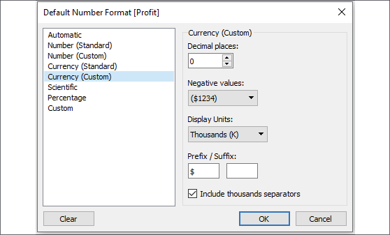
Figure 2.19: Editing the default number format of a field
- Right-click the Profit field again and select Default properties | Color.... The resulting dialog gives you an option to select and customize the default color encoding of the Profit field. Experiment with various palettes and settings. Notice that every time you click the Apply button, the visualization updates.
Diverging palettes (palettes that blend from one color to another) work particularly well for fields such as Profit, which can have negative and positive values. The default center of 0 allows you to easily tell what values are positive or negative based on the color shown.

Figure 2.20: Customizing color
Because you have set the default format for the field at the data-source level, any additional views you create using Profit will include the default formatting you specified.
Consider using color blind-safe colors in your visualizations. Orange and blue are usually considered a color blind-safe alternative to red and green. Tableau also includes a discrete color blind-safe palette. Additionally, consider adjusting the intensity of the colors, using labels, or different visualizations to make your visualizations more accessible.
Working with extracts instead of live connections
Nearly all data sources allow the option of either connecting live or extracting the data. A few cloud-based data sources require an extract. Conversely, OLAP data sources cannot be extracted and require live connections.
Extracts extend the way in which Tableau works with data. Consider the following diagram:

Figure 2.21: Data from the original Data Source is extracted into a self-contained snapshot of the data
When using a live connection, Tableau issues queries directly to the data source (or uses data in the cache, if possible). When you extract the data, Tableau pulls some or all of the data from the original source and stores it in an extract file. Prior to version 10.5, Tableau used a Tableau Data Extract (.tde) file. Starting with version 10.5, Tableau uses Hyper extracts (.hyper) and will convert .tde files to .hyper as you update older workbooks.
The fundamental paradigm of how Tableau works with data does not change, but you'll notice that Tableau is now querying and getting results from the extract. Data can be retrieved from the source again to refresh the extract. Thus, each extract is a snapshot of the data source at the time of the latest refresh. Extracts offer the benefit of being portable and extremely efficient.
Creating extracts
Extracts can be created in multiple ways, as follows:
- Select Extract on the Data Source screen as follows. The Edit... link will allow you to configure the extract:

Figure 2.22: Select either Live or Extract for a connection and configure options for the extract by clicking Edit.
- Select the data source from the Data menu, or right-click the data source on the data pane and select Extract data. You will be given a chance to set configuration options for the extract, as demonstrated in the following screenshot:

Figure 2.23: The Extract data… option
- Developers may create an extract using the Tableau Hyper API. This API allows you to use Python, Java, C++, or C#/.NET to programmatically read and write Hyper extracts. The details of this approach are beyond the scope of this book, but documentation is readily available on Tableau's website at https://help.tableau.com/current/api/hyper_api/en-us/index.html.
- Certain tools, such as
AlteryxorTableau Prep, can output Tableau extracts.
You'll have quite a few options for configuring an extract. To edit these options, select Extract and then Edit… on the Data Source screen or Extract data… from the context menu of a connection in the Data pane. When you configure an extract, you will be prompted to select certain options, as shown here:
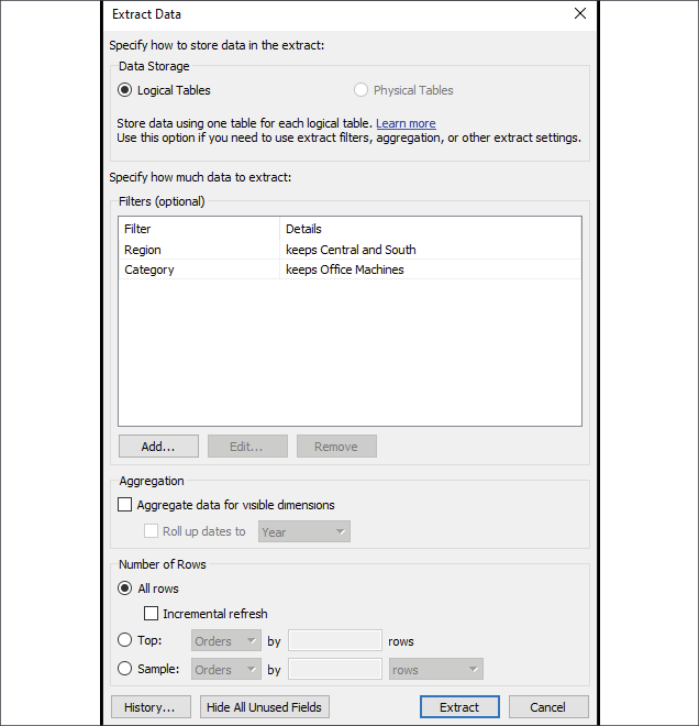
Figure 2.24: The Extract Data dialog gives quite a few options for how to configure the extract
You have a great deal of control when configuring an extract. Here are the various options, and the impact your choices will make on performance and flexibility:
- Depending on the data source and object model you've created, you may select between Logical Tables and Physical Tables. We'll explore the details in Chapter 13, Understanding the Tableau Data Model, Joins, and Blends.
- You may optionally add extract Filters, which limit the extract to a subset of the original source. In this example only, records where Region is Central or South and where Category is Office Machines will be included in the extract.
- You may aggregate an extract by checking the box. This means that data will be rolled up to the level of visible dimensions and, optionally, to a specified date level, such as year or month.
Visible fields are those that are shown in the data pane. You may hide a field from the Data Source screen or from the data pane by right-clicking a field and selecting Hide. This option will be disabled if the field is used in any view in the workbook.
Hiddenfields are not available to be used in a view.Hiddenfields are not included in an extract as long as they are hidden prior to creating or optimizing the extract.
In the preceding example, if only the Region and Category dimensions were visible, the resulting extract would only contain two rows of data (one row for Central and another for South). Additionally, any measures would be aggregated at the Region/Category level and would be done with respect to the Extract filters. For example, Sales would be rolled up to the sum of sales in Central/Office Machines and South/Office Machines. All measures are aggregated according to their default aggregation.
You may adjust the number of rows in the extract by including all rows or a sampling of the top n rows in the dataset. If you select all rows, you can indicate an incremental refresh. If your source data incrementally adds records, and you have a field such as an identity column or date field that can be used reliably to identify new records as they are added, then an incremental extract can allow you to add those records to the extract without recreating the entire extract. In the preceding example, any new rows where Row ID is higher than the highest value of the previous extract refresh would be included in the next incremental refresh.
Incremental refreshes can be a great way to deal with large volumes of data that grow over time. However, use incremental refreshes with care, because the incremental refresh will only add new rows of data based on the field you specify. You won't get changes to existing rows, nor will rows be removed if they were deleted at the source. You will also miss any new rows if the value for the incremental field is less than the maximum value in the existing extract.
Now that we've considered how to create and configure extracts, let's turn our attention to using them.
Performance
There are two types of extracts in Tableau:
- Tableau Data Extracts (
.tdefiles): prior to Tableau 10.5, these were the only type of extract available. - Hyper (
.hyperfiles) are available in Tableau 10.5 or later.
Depending on scale and volume, both .hyper and .tde extracts may perform faster than most traditional live database connections. For the most part, Tableau will default to creating Hyper extracts. Unless you are using older versions of Tableau, there is little reason to use the older .tde. The incredible performance of Tableau extracts is based on several factors, including the following:
- Hyper extracts make use of a hybrid of OLTP and OLAP models and the engine determines the optimal query. Tableau Data Extracts are columnar and very efficient to query.
- Extracts are structured so they can be loaded quickly into memory without additional processing and moved between memory and disk storage, so the size is not limited to the amount of RAM available, but RAM is efficiently used to boost performance.
- Many calculated fields are materialized in the extract. The pre-calculated value stored in the extract can often be read faster than executing the calculation every time the query is executed. Hyper extracts extend this by potentially materializing many aggregations.
You may choose to use extracts to increase performance over traditional databases. To maximize your performance gain, consider the following actions:
- Prior to creating the extract, hide unused fields. If you have created all desired visualizations, you can click the Hide Unused Fields button on the Extract dialog to hide all fields not used in any view or calculation.
- If possible, use a subset of data from the original source. For example, if you have historical data for the last 10 years but only need the last two years for analysis, then filter the extract by the
Datefield. - Optimize an extract after creating or editing calculated fields or deleting or hiding fields.
- Store extracts on solid-state drives.
Although performance is one major reason to consider using extracts, there are other factors to consider, which we will do next.
Portability and security
Let's say that your data is hosted on a database server accessible only from inside your office network. Normally, you'd have to be onsite or using a VPN to work with the data. Even cloud-based data sources require an internet connection. With an extract, you can take the data with you and work offline.
An extract file contains data extracted from the source. When you save a workbook, you may save it as a Tableau workbook (.twb) file or a Tableau Packaged Workbook (.twbx) file. Let's consider the difference:
- A Tableau workbook (
.twb) contains definitions for all the connections, fields, visualizations, and dashboards, but does not contain any data or external files, such as images. A Tableau workbook can be edited in Tableau Desktop and published to Tableau Server. - A Tableau packaged workbook (
.twbx) contains everything in a (.twb) file but also includes extracts and external files that are packaged together in a single file with the workbook. A packaged workbook using extracts can be opened with Tableau Desktop, Tableau Reader, and published to Tableau Public or Tableau Online.
A packaged workbook file (.twbx) is really just a compressed .zip file. If you rename the extension from .twbx to .zip, you can access the contents as you would any other .zip file.
There are a couple of security considerations to keep in mind when using an extract. First, any security layers that limit which data can be accessed according to the credentials used will not be effective after the extract is created. An extract does not require a username or password. All data in an extract can be read by anyone. Second, any data for visible (non-hidden) fields contained in an extract file (.hyper or .tde), or an extract contained in a packaged workbook (.twbx), can be accessed even if the data is not shown in the visualization. Be very careful to limit access to extracts or packaged workbooks containing sensitive or proprietary data.
When to use an extract
You should consider various factors when determining whether to use an extract. In some cases, you won't have an option (for example, OLAP requires a live connection and some cloud-based data sources require an extract). In other cases, you'll want to evaluate your options.
In general, use an extract when:
- You need better performance than you can get with the live connection.
- You need the data to be portable.
- You need to use functions that are not supported by the database data engine (for example,
MEDIANis not supported with a live connection to SQL Server). - You want to share a packaged workbook. This is especially true if you want to share a packaged workbook with someone who uses the free Tableau Reader, which can only read packaged workbooks with data extracted.
In general, do not use an extract when you have any of the following use cases:
- You have sensitive data that should not be accessible by certain users, or you have no control over who will be able to access the extract. However, you may hide sensitive fields prior to creating the extract, in which case they are no longer part of the extract.
- You need to manage security based on login credentials. (However, if you are using Tableau Server, you may still use extracted connections hosted on Tableau Server that are secured by a login. We'll consider sharing your work with Tableau Server in Chapter 16, Sharing Your Data Story).
- You need to see changes in the source data updated in real time.
- The volume of data makes the time required to build the extract impractical. The number of records that can be extracted in a reasonable amount of time will depend on factors such as the data types of fields, the number of fields, the speed of the data source, and network bandwidth. The Hyper engine typically builds
.hyperextracts much faster than the older.tdefiles were built.
With an understanding of how to create, manage, and use extracts (and when not to use them), we'll turn our attention to various ways of filtering data in Tableau.
Filtering data
Often, you will want to filter data in Tableau in order to perform an analysis on a subset of data, narrow your focus, or drill into details. Tableau offers multiple ways to filter data.
If you want to limit the scope of your analysis to a subset of data, you can filter the data at the source using one of the following techniques:
- Data Source Filters are applied before all other filters and are useful when you want to limit your analysis to a subset of data. These filters are applied before any other filters.
- Extract Filters limit the data that is stored in an extract (
.tdeor.hyper). Data source filters are often converted into extract filters if they are present when you extract the data. - Custom SQL Filters can be accomplished using a live connection with custom SQL, which has a Tableau parameter in the
WHEREclause. We'll examine parameters in Chapter 4, Starting an Adventure with Calculations and Parameters.
Additionally, you can apply filters to one or more views using one of the following techniques:
- Drag and drop fields from the data pane to the Filters shelf.
- Select one or more marks or headers in a view and then select Keep Only or Exclude, as shown here:

Figure 2.25: Based on the mark selection, you may Keep Only values that match or Exclude such values.
- Right-click any field in the data pane or in the view and select Show Filter. The filter will be shown as a control (examples include a drop-down list and checkbox) to allow the end user of the view or dashboard the ability to change the filter.
- Use an action filter. We'll look more at filters and action filters in the context of dashboards.
Each of these options adds one or more fields to the Filters shelf of a view. When you drop a field on the Filters shelf, you will be prompted with options to define the filter. The filter options will differ most noticeably based on whether the field is discrete or continuous. Whether a field is filtered as a dimension or as a measure will greatly impact how the filter is applied and the results.
Filtering discrete (blue) fields
When you filter using a discrete field, you will be given options for selecting individual values to keep or exclude. For example, when you drop the discrete Department dimension onto the Filters shelf, Tableau will give you the following options:
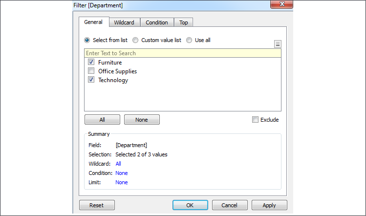
Figure 2.26: A filter for a discrete field will show options for including or excluding individual values
The Filter options include General, Wildcard, Condition, and Top tabs. Your filter can include options from each tab. The Summary section on the General tab will show all options selected:
- The General tab allows you to select items from a list (you can use the custom list to add items manually if the dimension contains a large number of values that take a long time to load). You may use the Exclude option to exclude the selected items.
- The Wildcard tab allows you to match string values that contain, start with, end with, or exactly match a given value.
- The Condition tab allows you to specify conditions based on aggregations of other fields that meet conditions (for example, a condition to keep any Department where the sum of sales was greater than $1,000,000). Additionally, you can write a custom calculation to form complex conditions. We'll cover calculations more in Chapter 4, Starting an Adventure with Calculations and Parameters, and Chapter 6, Diving Deep with Table Calculations.
- The Top tab allows you to limit the filter to only the top or bottom items. For example, you might decide to keep only the top five items by the sum of sales.
Discrete measures (except for calculated fields using table calculations) cannot be added to the Filters shelf. If the field holds a date or numeric value, you can convert it to a continuous field before filtering. Other data types will require the creation of a calculated field to convert values you wish to filter into continuous numeric values.
Let's next consider how continuous filters are filtered.
Filtering continuous (green) fields
If you drop a continuous dimension onto the Filters shelf, you'll get a different set of options. Often, you will first be prompted as to how you want to filter the field, as follows:
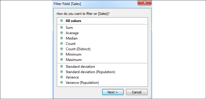
Figure 2.27: For numeric values, you'll often see options for aggregating the value as part of the filter
The options here are divided into two major categories:
- All values: The filter will be based on each individual value of the field, row by row. For example, an All values filter keeping only sales above $100 will evaluate each record of underlying data and keep only individual sales above $100.
- Aggregation: The filter will be based on the aggregation specified (for example, Sum, Average, Minimum, Maximum, Standard deviation, and Variance) and the aggregation will be performed at the level of detail of the view. For example, a filter keeping only the sum of sales above $100,000 on a view at the level of category will keep only categories that had at least $100,000 in total sales.
Once you've made a selection (or if the selection wasn't applicable for the field selected), you will be given another interface for setting the actual filter, as follows:
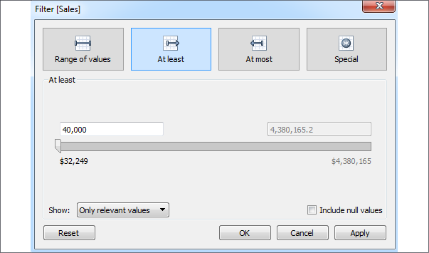
Figure 2.28: Filter options for Sales (as a SUM)
Here, you'll see options for filtering continuous values based on a range with a start, end, or both. The Special tab gives options for showing all values, NULL values, or non-NULL values.
From a user-interface perspective, the most dramatic difference in filtering options comes from whether a field is discrete or continuous. However, you should always think about whether you are using the field as a Dimension Filter or a Measure Filter to understand what kind of results you will get based on the order of operations, which is discussed in the Appendix.
- Dimension filters will filter detail rows of data. For example, filtering out the Central Region will eliminate all rows for that region. You will not see any states for that region and your aggregate results, such as
SUM(Sales), will not include any values from that region. - Measure filters will filter aggregate rows of data at the level of detail defined by the dimensions included in your view. For example, if you filtered to include only where
SUM(Sales)was greater than $100,000 and your view includedRegionandMonth, then the resulting view would include only values where theRegionhad more than $100,000 in sales for the given month.
Other than filtering discrete and continuous fields, you'll also notice some different options for filtering dates, which we'll consider next.
Filtering dates
We'll take a look at the special way Tableau handles dates in the Visualizing dates and times section of Chapter 3, Moving Beyond Basic Visualizations. For now, consider the options available when you drop an Order Date field onto the Filters shelf, as follows:
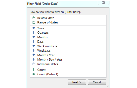
Figure 2.29: Initial filter options for a date field
The options here include the following:
- Relative date: This option allows you to filter a date based on a specific date (for example, keeping the last three weeks from today, or the last six months from January 1).
- Range of dates: This option allows you to filter a date based on a range with a starting date, ending date, or both.
- Date Part: This option allows you to filter based on discrete parts of dates, such as Years, Months, Days, or combinations of parts, such as Month/Year. Based on your selection, you will have various options for filtering and have the option of defaulting to the latest value in the data.
- Individual dates: This option allows you to filter based on each individual value of the date field in the data.
- Count or Count (Distinct): This option allows you to filter based on the count, or distinct count, of date values in the data.
Depending on your selection, you will be given additional options for filtering.
Other filtering options
You will also want to be aware of the following options when it comes to filtering:
- You may display a filter control for nearly any field by right-clicking it and selecting Show Filter. The type of control depends on the type of field, whether it is discrete or continuous, and may be customized by using the little drop-down arrow at the upper-right of the filter control.
- Filters may be added to the context. Context is described in detail in the Appendix and we'll see why it's important in various examples throughout the book. For now, just note the option. This option is available via the drop-down menu on the filter control or the field on the Filters shelf.
- Filters may be set to show all values in the database, all values in the context, all values in a hierarchy, or only values that are relevant based on other filters. These options are available via the drop-down menu on the Filter control or the field on the Filters shelf.
- When using Tableau Server, you may define user filters that allow you to provide row-level security by filtering based on user credentials.
- By default, any field placed on the Filters shelf defines a filter that is specific to the current view. However, you may specify the scope by using the menu for the field on the Filters shelf. Select Apply to and choose one of the following options:
- All related data sources: All data sources will be filtered by the value(s) specified. The relationships of fields are the same as blending (that is, the default by name and type match, or customized through the Data | Edit Relationships... menu option). All views using any of the related data sources will be affected by the filter. This option is sometimes referred to as cross-data source filtering.
- Current data source: The data source for that field will be filtered. Any views using that data source will be affected by the filter.
- Selected worksheets: Any worksheets selected that use the data source of the field will be affected by the filter.
- Current worksheet: Only the current view will be affected by the filter.
We'll see plenty of practical examples of filtering data throughout the book, many of which will make use of some of these options.
Summary
This chapter covered key concepts of how Tableau works with data. Although you will not usually be concerned with what queries Tableau generates to query underlying data engines, having a solid understanding of Tableau's paradigm will greatly aid you as you analyze data.
We looked at multiple examples of different connections to different data sources, considered the benefits and potential drawbacks of using data extracts, considered how to manage metadata, and considered options for filtering data.
Working with data is fundamental to everything you do in Tableau. Understanding how to connect to various data sources, when to work with extracts, and how to customize metadata will be key as you begin deeper analysis and more complex visualizations, such as those covered in Chapter 3, Moving Beyond Basic Visualizations.