Chapter 7: Supervised Machine Learning

As you begin to progress your career and skill set in the field of data science, you will encounter many different types of models that fall into one of the two categories of either supervised or unsupervised learning. Recall that in applications of unsupervised learning, models are generally trained to either cluster or transform data in order to group or reshape data to extract insights when labels are not available for the given dataset. Within this chapter, we will now discuss the applications of supervised learning as they apply to the areas of classification and regression to develop powerful predictive models to make educated guesses about a dataset's labels.

Over the course of this chapter, we will discuss the following topics:

• Understanding supervised learning
• Measuring success in supervised machine learning
• Understanding classification in supervised machine learning
• Understanding regression in supervised machine learning

With our objectives in mind, let's now go ahead and get started.

Understanding supervised learning

As you begin to explore data science either on your own or within an organization, you will often be asked the question, What exactly does supervised machine learning mean? Let's go ahead and come up with a definition. We can define supervised learning as a general subset of machine learning in which data, like its associated labels, is used to train models that can learn or generalize from the data to make predictions, preferably with a high degree of certainty. Thinking back to Chapter 5, Introduction to Machine Learning, we can recall the example we completed concerning the breast cancer dataset in which we classified tumors as being either malignant or benign. This example, alongside the definition we created, is an excellent way to learn and understand the meaning behind supervised learning.

With the definition of supervised machine learning now in our minds, let's go ahead and talk about its different subtypes, namely, classification and regression. If you recall, classification within the scope of machine learning is the act of predicting a category for a given set of data, such as classifying a tumor as malignant or benign, an email as spam or not spam, or even a protein as alpha or beta. In each of these cases, the model will output a discrete value. On the other hand, regression is the prediction of an exact value using a given set of data, such as the lipophilicity of a small molecule, the isoelectric point of a Monoclonal Antibody (mAb), or the LCAP of an LCMS peak. In each of these cases, the model will output a continuous value.

Many different models exist within the two categories of supervised learning. Within the scope of this book, we will focus on four main models for each of these two categories. When it comes to classification, we will discuss K-Nearest Neighbor (KNN), Support Vector Machines (SVMs), decision trees, and random forests, as well as XGBoost classification. When it comes to regression, we will discuss linear regression, logistic regression, random forest regression, and even gradient boosting regression. We can see these depicted in Figure 7.1:

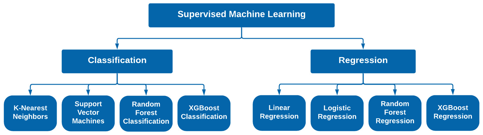
Figure 7.1 – The two areas of supervised machine learning

Our main objective in each of these models is to train a new instance of that model for a particular dataset. We will fit our model with the data, and tune or adjust the parameters to give us the best outcomes. To determine what the best outcomes should be, we will need to know how to measure success within our models. We will learn about that in the following section.

Measuring success in supervised machine learning

As we begin to train our supervised classifiers and regressors, we will need to implement a few ways to determine which models are performing better, thus allowing us to effectively tune the model's parameters and maximize its performance. The best way to achieve this is to understand what success looks like ahead of time before diving into the model development process. There are many different methods for measuring success depending on the situation. For example, accuracy can be a good metric for classifiers, but not regressors. Similarly, a business case for a classifier may not necessarily require accuracy to be the primary metric of interest. It simply depends on the situation at hand. Let's take a look at some of the most common metrics used for each of the fields of classification and regression.

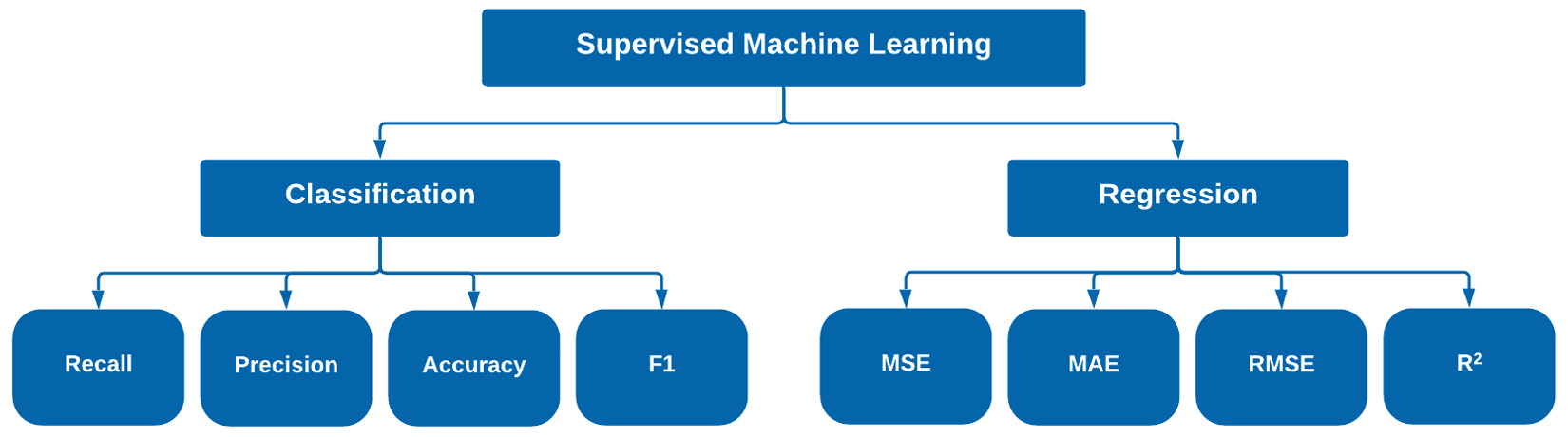
Figure 7.2 – Common success metrics for regression and classification

Although there are many other metrics you can use for a given scenario, the eight listed in Figure 7.2 are some of the most common ones you will likely encounter. Selecting a given metric can be difficult as it should always align with the given use case. Let's go ahead and explore this when it comes to classification.

Measuring success with classifiers

Take, for example, the tumor dataset we have worked with thus far. We defined our success metric as accuracy, and therefore maximizing accuracy was our model's main training objective. This, however, is not always the case, and the success metric you choose to use will almost always be dependent on both the model and the business problem at hand. Let's go ahead and take a closer look at some metrics commonly used in the data science space and define them:

• Accuracy: A measurement that agrees closely with the accepted value
• Precision: A measurement that agrees with other measurements in the sense that they are similar to one another

An easier way to think about accuracy and precision is by picturing the results displayed using a bullseye depiction. The difference between precision and accuracy is in the sense of both how close the results are to one another, and how close the results are to their true or actual values, respectively. We can see a visual depiction of this in Figure 7.3:

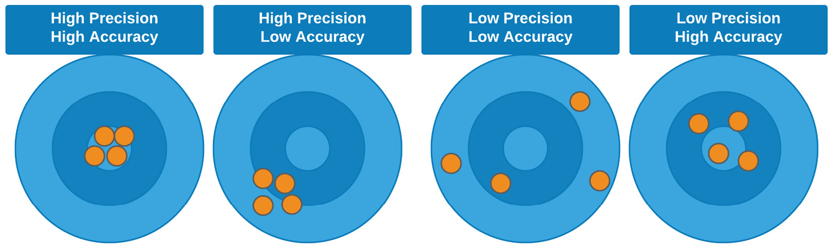
Figure 7.3 – Graphical illustration of the difference between accuracy and precision

In addition to the visual depiction, we can also think of precision as a calculation representing the results as subsets relative to a total population. In this case, we will also need to define a new metric known as recall. We can think of recall and precision mathematically in the context of positive and negative results through what is known as a confusion matrix. When comparing the results of a prediction relative to the actual results, we can get a good sense of the model's performance by comparing a few of these values. We can see a visual depiction of this in Figure 7.4:

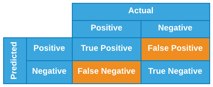
Figure 7.4 – Graphical illustration of a confusion matrix

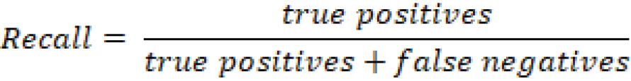
With this table in mind, we can define recall as the fraction of fraudulent cases that a given model identifies, or, from a mathematical perspective, we can define it as follows:

Whereas we can define precision in the same context as follows:

We can visualize accuracy, precision, and recall in a similar manner in the following diagram, in which each metric represents a specific calculation of the overall results:

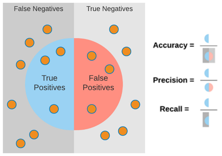
Figure 7.5 – Graphical illustration explaining accuracy, precision, and recall

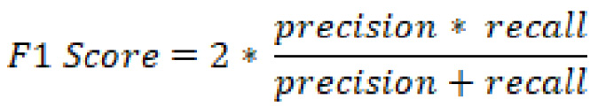
Finally, there is one last commonly used metric that is usually considered to be a loose combination of precision and recall known as the F1 score. We can define the F1 score as follows:

So how do you determine which metric to use? There is no best metric that you should always use as it is highly dependent on each situation. When determining the best metric, you should always ask yourself, What is the main objective for the model, as well as the business? In the eyes of the model, accuracy may be the best metric. On the other hand, in the eyes of the business, recall may be the best metric.

Ultimately, recall could be considered more useful when overlooked cases (defined above as false negatives) are more important. Consider, for example, a model that is predicting a patient's diagnosis – we would likely care more about false negatives than false positives. On the other hand, precision can be more important when false positives are more costly to us. It all depends on the given business case and requirements. So far, we have investigated success as it relates to classification, so let's now investigate these ideas as they relate to regression.

Measuring success with regressors

Although we have not yet taken a deep dive into the field of regression, we have defined the main idea as the development of a model whose output is a continuous numerical value. Take, for example, the molecular toxicity dataset containing many columns of data whose values are all continuous floats. Hypothetically, you could use this dataset to make predictions on the Total Polar Surface Area (TPSA). In this case, the metrics of accuracy, precision, and recall would not be the most useful to us to best understand the performance of our models. Alternatively, we will need some metrics better catered to continuous values.

One of the most common metrics for defining success in many models (not necessarily machine learning) is the Pearson correlation coefficient, also known as R2. This calculation is a common method used to measure the linearity of data, as it represents the proportion of variance in the dependent variable. We can define R2 as follows:

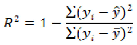
In this equation, is the predicted value, and is the mean value.

Take, for example, a dataset in which experimental (actual) values were known, and predicted values were calculated. We could plot the graphs of these values against one another and measure the correlation. In theory, a perfect model would have an ideal correlation (as close to a value of 1.00 as possible). We can see a depiction of high and low correlation in Figure 7.6:

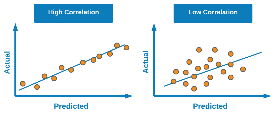
Figure 7.6 – Difference between high and low correlation in scatter plots

Although this metric can give you a good estimate of a model's performance, there are a few others that can give you a better sense of the model's error: Mean Absolute Error (MAE), Mean Squared Error (MSE), and Root Mean Squared Error (RMSE). Let's go ahead and define these:

• MAE: The average of the absolute differences between the actual and predicted values in a given dataset. This measure tends to be more robust when handling datasets with outliers:
  

  In which is the predicted value, and is the mean value.

• MSE: The average of the squared differences between the actual and predicted values in a given dataset:
  
• RMSE: Square root of the MSE to measure the standard deviation of the values. This metric is commonly used to compare regression models against each other:
  

When it comes to regression, there are many different metrics you can use depending on the given situation. In most regression models, RMSE is generally used to compare the performance of multiple models as it is quite simple to calculate and differentiable. On the other hand, datasets with outliers are generally compared to one another using MSE and MAE. Now that we have gained a better sense of measuring success through various metrics, let's now go ahead and explore the area of classification.

Understanding classification in supervised machine learning

Classification models in the context of machine learning are supervised models whose objectives are to classify or categorize items based on previously learned examples. You will encounter classification models in many forms as they tend to be some of the most common models used in the field of data science. There are three main types of classifiers that we can develop based on the outputs of the model.

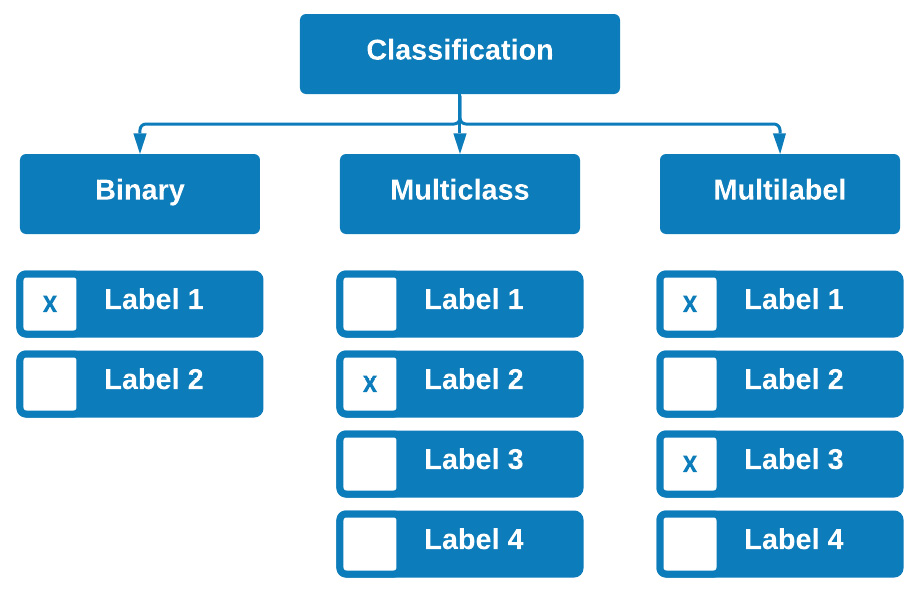
Figure 7.7 – The three types of supervised classification

The first type is known as a binary classifier. As the name suggests, this is a classifier that predicts in a binary fashion in the sense that an output is one of two options, such as emails being spam or not spam, or molecules being toxic or not toxic. There is no third option in either of these cases, rendering the model a binary classifier.

The second type of classifier is known as a multiclass classifier. This type of classifier is trained on more than two different outputs. For example, many types of proteins can be classified based on structure and function. Some of these examples include structural proteins, enzymes, hormones, storage proteins, and toxins. Developing a model that would predict the type of protein based on some of the protein's characteristics would be regarded as a multiclass classifier in the sense that each row of data could have only one possible class or output.

Finally, we also have multilabel classifiers. These classifiers, unlike their multiclass counterparts, are able to predict multiple outputs for a given row of data. For example, when screening patients for clinical trials, you may want to build patient profiles using many different types of labels, such as gender, age, diabetic status, and smoker status. When trying to predict what a certain group of patients might look like, we need to be able to predict all of these labels.

Now that we have broken down classification into a few different types, you are likely thinking about the many different areas in projects you are working on where a classifier may be of great value. The good news here is that many of the standard or popular classification models we are about to explore can be easily recycled and fitted with new data. As we begin to explore the many different models in the following section, think about the projects that you are working on and the datasets you have available, and which models they may fit the best.

Exploring different classification models

As we explore a number of machine learning models, we will test out their performances on a new dataset concerning single-cell RNA sequences, published by Nestorowa et al. in 2016. We will focus on using this structured dataset in order to develop a number of different classifiers. Let's go ahead and import the data and prepare it for the classification models. First, we will go ahead and import our dataset of interest using the read_csv() function in pandas:

dfx = pd.read_csv("../../datasets/single_cell_rna/nestorowa_corrected_log2_transformed_counts.txt", sep=' ',  )

Next, we will use the index to isolate our labels (classes) for each of the rows, using the first four characters of each row:

dfx['annotation'] = dfx.index.str[:4]

y = dfx["annotation"].values.ravel()

We can use the head() function to take a look at the data. What we will notice is that there is more than 3,992 columns' worth of data. As any good data scientist knows, developing models with too many columns will lead to many inefficiencies, and therefore it would be best to reduce these down using an unsupervised learning technique, such as PCA. Prior to applying PCA, we will need to scale or normalize our dataset using the StandardScaler class in sklearn:

from sklearn.preprocessing import StandardScaler

scaler = StandardScaler()

X_scaled = scaler.fit_transform(dfx.drop(columns = ["annotation"]))

Next, we can apply PCA to reduce our dataset from 3,992 columns down to 15:

from sklearn.decomposition import PCA

pca = PCA(n_components=15, svd_solver='full')

pca.fit(X_scaled)

data_pca = pca.fit_transform(X_scaled)

With the data now in a much more reduced state, we can check the explained variance ratio to see how this compares with the original dataset. We will see that the sum of all columns totals 0.17, which is relatively low. We will want to aim for a value around 0.8, so let's go ahead and increase the total number of columns in order to increase the percentage of variance:

pca = PCA(n_components=900, svd_solver='full')

pca.fit(X_scaled)

data_pca = pca.fit_transform(X_scaled)

With the PCA model applied, we managed to reduce the total number of columns by roughly 77%.

With this completed, we are now prepared to split our dataset using the train_test_split() class:

from sklearn.model_selection import train_test_split

X_train, X_test, y_train, y_test = train_test_split(data_pca, y, test_size=0.33)

With the dataset now split into training and test sets, we are now ready to begin the classification model development process!

K-Nearest Neighbors

One of the classic, easy-to-develop, and most commonly discussed classification models is known as the KNN model, first developed by Evelyn Fix and Joseph Hodges in 1951. The main idea behind this model is determining class membership based on proximity to the closest neighbors. Take, for example, a 2D binary dataset in which items are classified as either A or B. As a new dataset is added, the model will determine its membership or class based on its proximity (usually Euclidean) to other items in the same dataset.

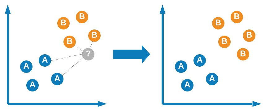
Figure 7.8 – Graphical representation of the KNN model

KNN is regarded as one of the easiest machine learning models to develop and implement given its simple nature and clever design. The model, although simple in application, does require some tuning in order to be fully effective. Let's go ahead and explore the use of this model for the single-cell RNA classification dataset:

1. We can begin by importing the KNeighborsClassifier model from sklearn:

   from sklearn.neighbors import KNeighborsClassifier

2. Next, we can instantiate a new instance of this model in Python, the number of neighbors to a value of 5, and fit the model to our training data:

   knn = KNeighborsClassifier(n_neighbours=5)

   knn.fit(X_train, y_train)

3. With the model fit, we can now go ahead and predict the outcomes of the model and set those to a variable we will call y_pred, and finally use the classification_report function to see the results:

   y_pred = knn.predict(X_test)

   print(classification_report(y_test, y_pred))

   Using the classification report function, we can get a sense of the precision, recall, and F1 scores for each of the three classes. We can see that the precision was relatively high for the LT.H class, but slightly lower for the other two. Alternatively, recall was very low for the LT.H class, but quite high for the Prog class. In total, an average precision of 0.63 was calculated for this model:

   

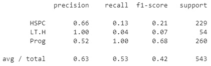
   Figure 7.9 – Results of the KNN model

   With these results in mind, let's go ahead and tune one of the parameters, namely, the n_neighbours parameter in the range of 1-10.

4. We can use a simple for loop to accomplish this:

   for i in range(1,10):

       knn = KNeighborsClassifier(n_neighbors=i)

       knn.fit(X_train, y_train)

       y_pred = knn.predict(X_test)

       print("n =", i, "acc =", accuracy_score(y_test, y_pred))

   If we take a look at the results, we can see the number of neighbors as well as the overall model accuracy. Immediately, we notice that the option value based on this metric alone is n=2, giving an accuracy of approximately 60%.

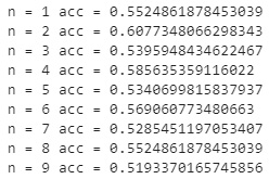
Figure 7.10 – Results of the KNN model at different neighbors

KNN is one of the simplest and fastest models for the development of classifiers; however, it is not always the best model for a complex dataset such as this one. You will notice that the results varied heavily from class to class, indicating the model was not able to effectively distinguish between them based on their proximity to other members alone. Let's go ahead and explore another model known as an SVM, which tries to classify items in a slightly different way.

Support Vector Machines

SVMs are a class of supervised machine learning models commonly used for both classification and regression, first developed in 1992 by AT&T Bell Laboratories. The main idea behind SVMs is the ability to separate classes using a hyperplane. There are three main types of SVMs that you will likely hear about in discussions or encounter in the data science field: linear SVMs, polynomial SVMs, and RBF SVMs.

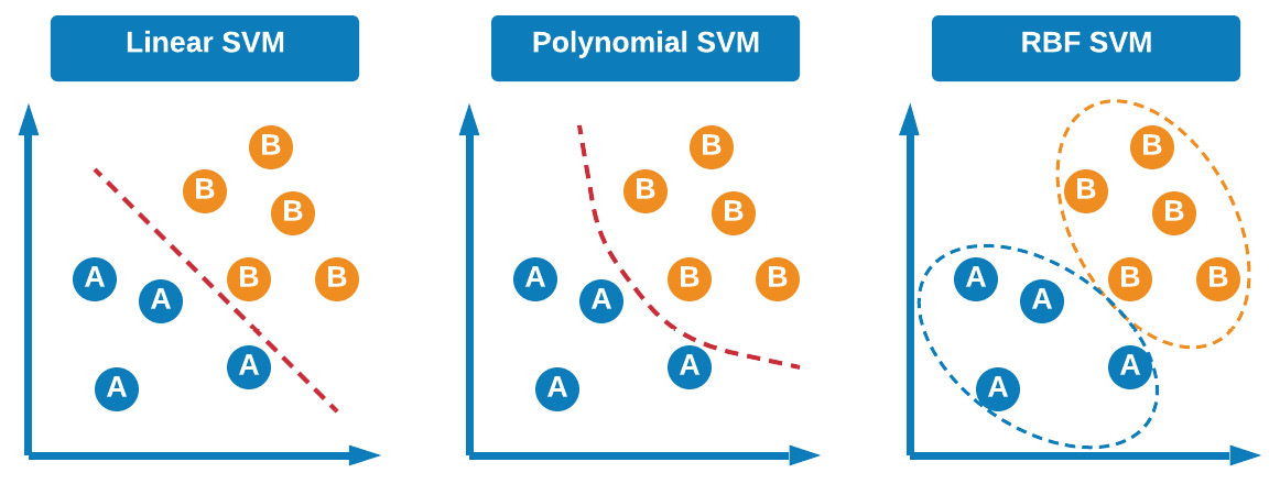
Figure 7.11 – Visual explanation of the different SVMs

The main idea behind the three models lies in how the classes are separated. For example, in linear models, the hyperplane is a linear line separating the two classes from each other. Alternatively, the hyperplane may consist of a polynomial, allowing the model to account for non-linear features. Finally, and most popularly, the model can use a Radial Basis Function (RBF) to determine a datapoint's membership, which is based on two parameters, gamma and C, which account for the decision region, how it is spread out, and the penalty for a misclassification. With this in mind, let's now take a closer look at the idea of a hyperplane.

The hyperplane is a function that attempts to clearly define and allow for the differentiation between classes in either a linear or non-linear fashion. The hyperplane can be described mathematically as follows:

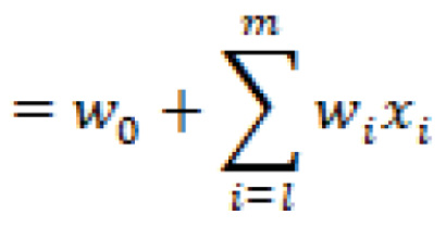
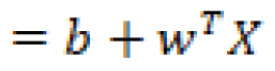
In which are the vectors, is the bias term, and are the variables.

Taking a quick break from the RNA dataset, let's go ahead and demonstrate the use of a linear support vector using the enrollment dataset in Python – a dataset concerning patient enrolment in which respondent data was summarized via PCA into two features. The three possible labels within this dataset are Likely, Very Likely, or Unlikely to enroll. The main objective of a linear SVM is to draw a line clearly separating the data based on class.

Before we begin using SVM, let's go ahead and import our dataset:

df = pd.read_csv("../datasets/dataset_enrollment_sd.csv")

For simplicity, let's eliminate the Likely class and keep the Very Likely and Unlikely classes:

dftmp = df[(df["enrollment_cat"] != "Likely")]

Let's go ahead and draw a line separating the data shown in the scatter plot:

     plt.figure(figsize=(15, 6))

     xfit = np.linspace(-90, 130)

         sns.scatterplot(dftmp["Feature1"],

                         dftmp["Feature2"],

                         hue=dftmp["enrollment_cat"].values,

                         s=50)

         for m, b in [(1, -45),]:

             plt.plot(xfit, m * xfit + b, '-k')

         plt.xlim(-120, 150);

         plt.ylim(-100, 60);

Upon executing this code, this yields the following diagram:

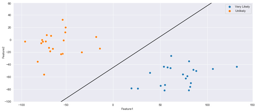
Figure 7.12 – Two clusters separated by an initial SVM hyperplane

Notice within the plot that this linear line could be drawn in multiple ways with different slopes, yet still successfully separate the two classes within the dataset. However, as new datapoints begin to encroach toward the middle ground between the two clusters, the slope and location of the hyperplane will begin to grow in importance. One way to address this issue is by defining the slope and location of the plane based on the closest datapoints. If the line contained a margin of width x in relation to the closest datapoints, then a more improved hyperplane could be constructed. We can construct this using the fill_between function, as portrayed in the following code:

         plt.figure(figsize=(15, 6))

         xfit = np.linspace(-110, 180)

         sns.scatterplot(dftmp["Feature1"],

                         dftmp["Feature2"],

                         hue=dftmp["enrollment_cat"].values,

                         s=50)

         for m, b, d in [(1, -45, 60),]:

      yfit = m * xfit + b

      plt.plot(xfit, yfit, '-k')

         plt.fill_between(xfit, yfit - d,

                     yfit + d, edgecolor='none',

                              color='#AAAAAA', alpha=0.4)

         plt.xlim(-120, 150);

         plt.ylim(-100, 60);

Upon executing this code, this yields the following figure:

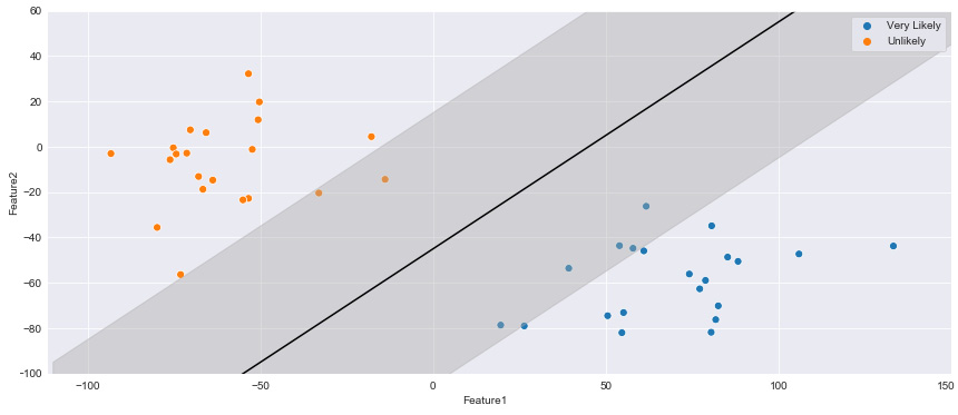
Figure 7.13 – Two clusters separated by an initial SVM hyperplane with specified margins

The datapoints from both classes that are within the margin width of the hyperplane are known as support vectors. The main intuition is the idea that the further away the support vectors are from the hyperplane, the higher the probability that a correct class is identified for a new datapoint.

We can train a new SVM classifier using the SVC class from the scikit-learn library. We begin by importing the class, splitting the data, and then training a model using the dataset:

from sklearn.model_selection import train_test_split

X_train, X_test, y_train, y_test =  

                train_test_split(dftmp[["Feature1","Feature2"]],

                                  dftmp["enrollment_cat"].values,

                                  test_size = 0.25)

from sklearn.svm import SVC

model = SVC (kernel='linear', C=1E10, random_state = 42)

model.fit(X_train, y_train)

With that, we have now fitted our model to the dataset. As a final step, we can show the scatter plot, identify the hyperplane, and also specify which datapoints were the support vectors for this particular example:

     plt.figure(figsize=(15, 6))

     sns.scatterplot(dftmp["Feature1"],

                     dftmp["Feature2"],

                     hue=dftmp["enrollment_cat"].values, s=50)

     plot_svc_decision_function(model);

     for j, k in model.support_vectors_:

         plt.plot([j], [k], lw=0, ='o', color='red',

                  markeredgewidth=2, markersize=20,

                  fillstyle='none')

Upon executing this code, this yields the following figure:

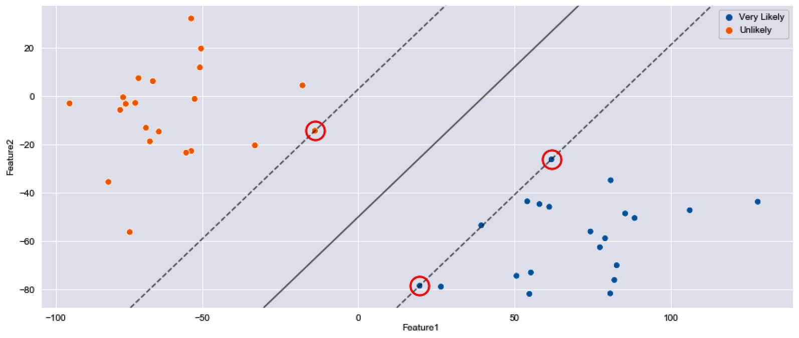
Figure 7.14 – Two clusters separated by an initial SVM hyperplane with select support vectors

Now that we have gained a better understanding of how SVMs operate in relation to their hyperplanes using this basic example, let's go ahead and test out this model using the single-cell RNA classification dataset we have been working with.

Following roughly the same steps as the KNN model, we will now implement the SVM model by first importing the library, instantiating the model with a linear kernel, fitting our training data, and subsequently making predictions on the test data:

from sklearn.svm import SVC

svc = SVC(kernel="linear")

svc.fit(X_train, y_train)

y_pred = svc.predict(X_test)

print(classification_report(y_test, y_pred))

Upon printing the report, this yields the following results:

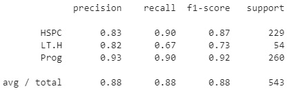
Figure 7.15 – Results of the SVM model

We can see that the model was, in fact, quite robust, with our dataset yielding some high metrics and giving us a total average precision of 88%. SVMs are fantastic models to use with complex datasets as their main objective is to separate data via a hyperplane. Let's now explore a model that takes a very different approach by using decision trees to arrive at final results.

Decision trees and random forests

Decision trees are one of the most popular and commonly used machine learning models when it comes to structured datasets for both classification and regression. Decision trees consist of three elements: nodes, edges, and leaf nodes.

Nodes generally consist of a question allowing for the process to split into an arbitrary number of child nodes, shown in orange in the following diagram. The root node is the first node that the entire tree is referenced through. Edges are the connections between nodes shown in blue. When nodes have no children, then this final destination is called a leaf, shown in green. In some cases, a decision tree will have nodes containing the same parent – these are called sibling nodes. The more nodes there are in a tree, the deeper the tree is said to be. The depth of the decision tree is a measure of complexity.

A tree that is not complex enough will not arrive at an accurate result, and a tree that is too complex will be overtrained. Identifying a good balance is one of the primary objectives in the training process. Using these elements, you can construct a decision tree, allowing for processes to flow from the top to the bottom, thereby arriving at a particular destination or decision:

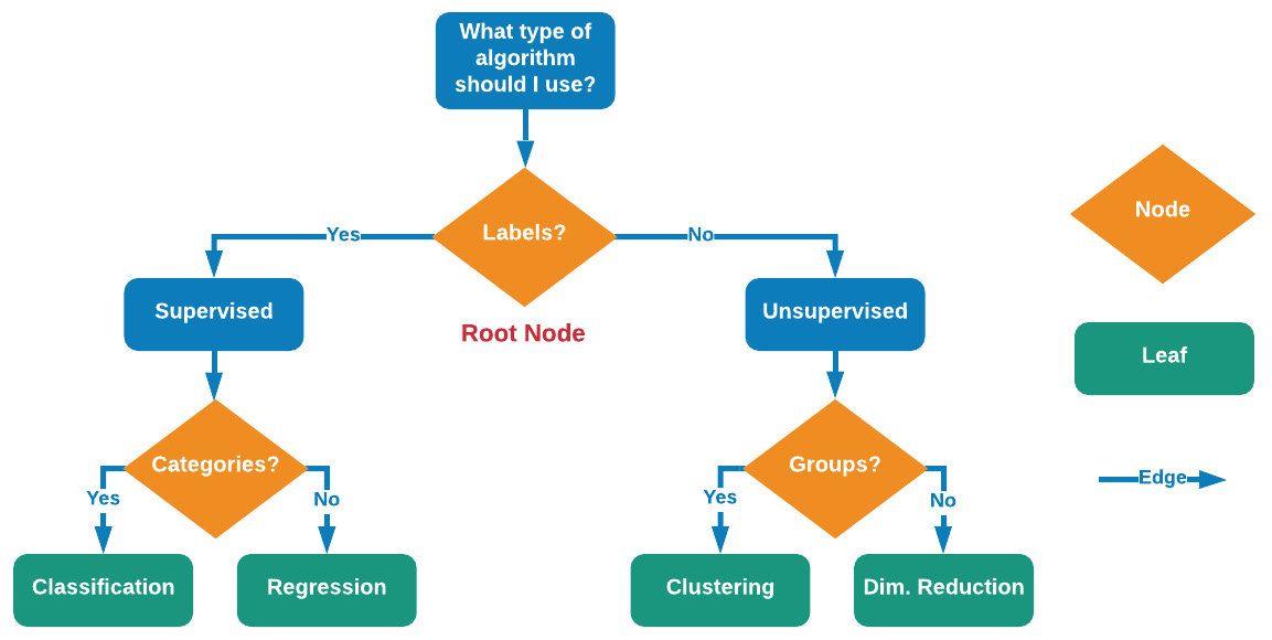
Figure 7.16 – Illustration of decision trees when it comes to nodes, leaves, and edges

Decision trees operate in quite a genius way. We begin with our initial dataset in which all datapoints are labeled and ready to go. The first objective is to split the dataset using a decision boundary that is the most informative – which, in this case, is at y=m. This has successfully isolated a class from the two others; however, the two others are still not yet isolated from one another. The algorithm then splits the dataset again at x = n, thus completely separating the three clusters. If more clusters were present, this process would iteratively and recursively continue until all classes are optimally separated. We can see a visual representation of this in Figure 7.17:

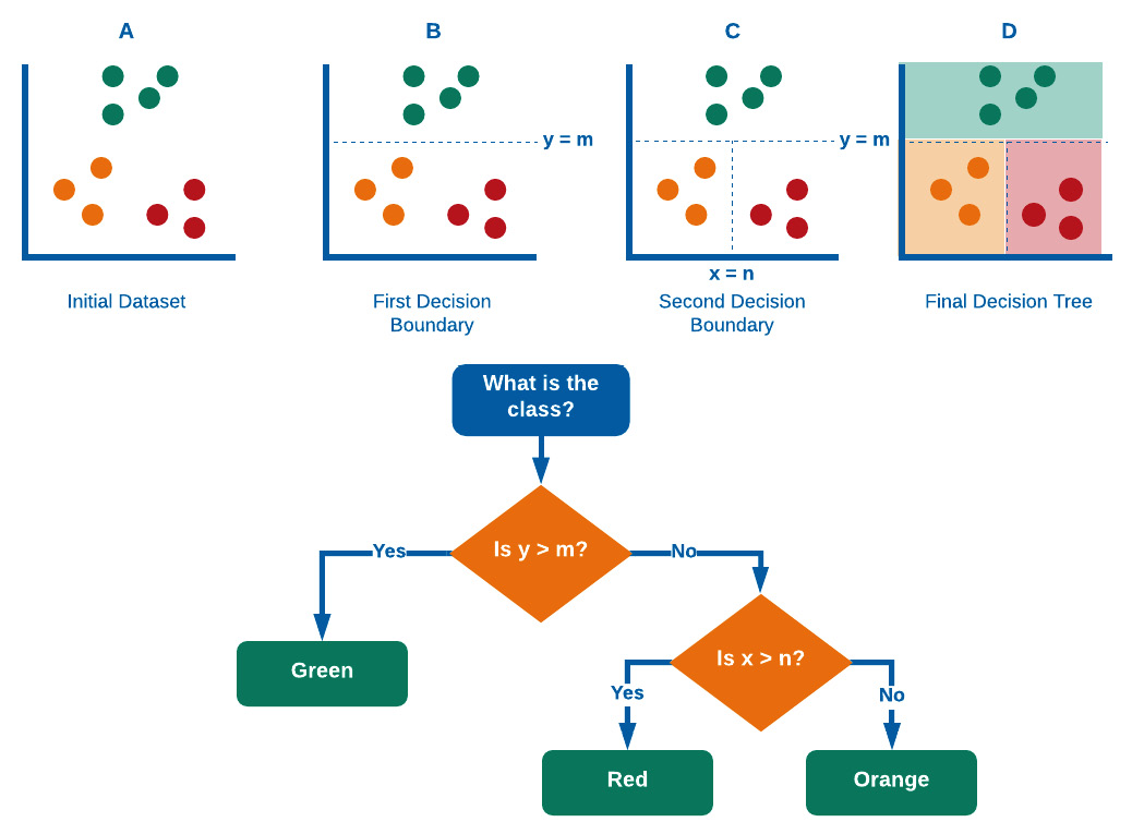
Figure 7.17 – A graphical representation of the process that decision trees take

Decision trees determine where and how to split the data using various splitting criteria, known as attribute selection measures. These prominent attribute selection measures include:

• Information gain
• Gain ratio
• Gini index

Let's now take a closer look at these three items.

Information gain is an attribute concerning the amount of information required to further describe the tree. This attribute minimizes the information needed for data classification while utilizing the least randomness in the partitions. Think of information gain of a random variable determined from the observation of a random variable, A, as a function such that:

Broadly speaking, the information gain is the change in entropy (information entropy) such that:

In which represents the conditional entropy of given the attribute . In summary, information gain answers the question, How much information do we obtain from this variable given another variable?

On the other hand, the gain ratio is the information gain relative to the intrinsic information. In other words, this measure is biased toward tests that result in many outcomes, thus forcing a preference in favor of features of this nature. The gain ratio can be represented as:

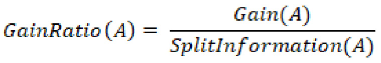
In which is represented as:

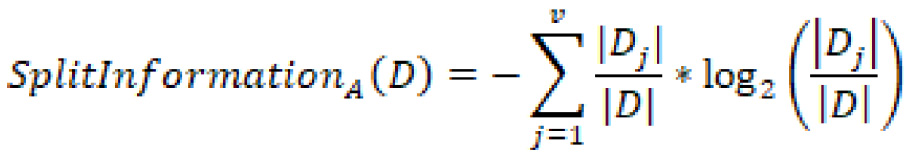
In summary, the gain ratio penalizes variables with more distinct values, which will help decide the next split at the next level.

Finally, we arrive at the Gini index, which is an attribute selection measure representing how often a randomly selected element is incorrectly labeled. The Gini index can be calculated by subtracting the sum of square probabilities of each class:

This methodology in determining a split naturally favors larger partitions as opposed to information gain, which favors smaller ones. The objective of any data scientist is to explore different methods with your dataset and determine the best path forward.

Now that we have a much more detailed explanation of decision trees and how the model operates, let's now go ahead and implement this model using the previous single-cell RNA classification dataset:

from sklearn.tree import DecisionTreeClassifier

dtc = DecisionTreeClassifier(max_depth=4)

dtc.fit(X_train, y_train)

y_pred = dtc.predict(X_test)

print(classification_report(y_test, y_pred))

Upon printing the report, this yields the following results:

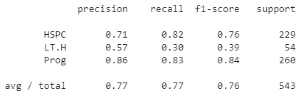
Figure 7.18 – Results of the decision tree classifier

We can see that the model, without any tuning, was able to deliver a total precision score of 77% using a max_depth value of 4. Using the same method as the KNN model, we can iterate over a range of max_depth values to determine the optimal value. Doing so would result in an ideal max_depth value of 3, yielding a total precision of 82%.

As we begin to train many of our models, one of the most common issues that we will face is overfitting our data in one way or another. Take, for example, a decision tree model that was very finely tuned for a specific selection of data since decision trees are built on an entire dataset using the features and variables of interest. In this case, the model may be prone to overfitting. On the other hand, another model known as a random forest is built using many different decision trees to help mitigate any potential overfitting.

Random forests are robust ensemble models based on decision trees. Where decision trees are generally designed to develop a model using the dataset as a whole, random forests randomly select features and rows and subsequently build multiple decision trees that are then averaged in their weights. Random forests are powerful models given their ability to limit overfitting while avoiding a substantial increase in error due to bias. We can see a visual representation of this in Figure 7.19:

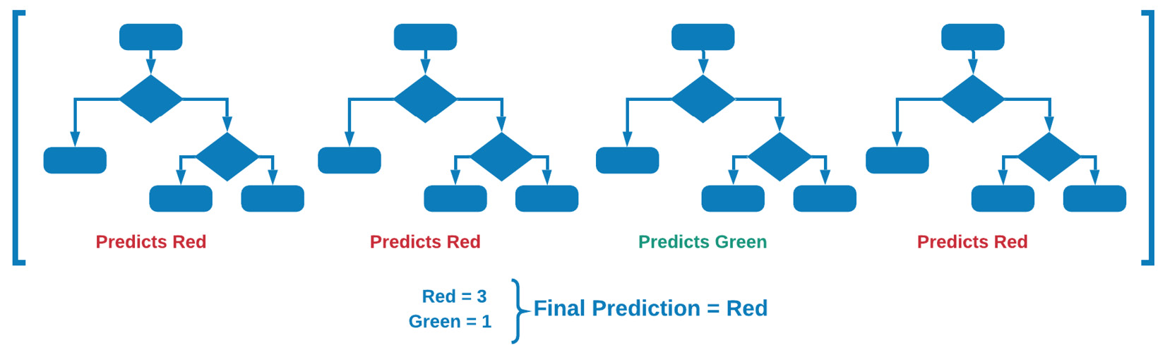
Figure 7.19 – Graphical explanation of random forest models

There are two main ways in which random forests can help reduce variance. The first method is by training on different samples of data. Consider the preceding example using the patient enrollment data. If the model was trained on samples not containing those in between the clusters, then determining the score on the test set will result in significantly lower accuracy.

The second method involves using a random subset of features to train on, allowing for the determination of the concept of feature importance within the model. Let's go ahead and take a look at this model using the single-cell RNA classification dataset:

from sklearn.ensemble import RandomForestClassifier

clf = RandomForestClassifier(n_estimators=1000)

clf.fit(X_train, y_train)

y_pred = clf.predict(X_test)

print(classification_report(y_test, y_pred))

Upon printing the report, this yields the following results:

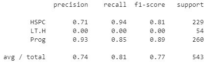
Figure 7.20 – Results of the random forest model

We can immediately observe that the model has a precision of roughly 74%, slightly lower than the decision tree above, indicating that the tree may have overfitted the data slightly.

Random forest models are very commonly used in the biotechnology and life sciences industries given their remarkable methods of avoiding overfitting, as well as their ability to develop predictive models with smaller datasets. Many applications of machine learning within the biotech space generally suffer from a concept known as the low-N problem, in the sense that use cases exist, but little to no data has been collected or organized with which to develop a model. Random forests are commonly used for applications in this space given their ensemble nature. Let's now take a look at a very different model that splits data not based on decisions, but based on statistical probability instead.

Extreme Gradient Boosting (XGBoost)

Over the last few years, a number of robust machine learning models have begun to enter the data science space, thus changing the machine learning landscape quite effectively – one of these models being the Extreme Gradient Boosting (XGBoost) model. The main idea behind this model is that it is an implementation of Gradient Boosted Models (GBMs), specifically, decision trees, in which speed and performance were highly optimized. Because of the highly efficient and highly effective nature of this model, it began to dominate many areas of data science and eventually became the go-to algorithm for many data science competitions on Kaggle.com.

There are many reasons why GBMs are so effective with structured/tabular datasets. Let's go ahead and explore three of these reasons:

• Parallelization: The XGBoost model implements a method known as parallelization. The main idea here is that it can parallelize processes in the construction of each of the trees. In essence, each of the branches of a single tree is trained separately.
• Tree-Pruning: Pruning is the process of removing parts of a decision tree deemed to be redundant or not useful to a model. The main idea behind GBM pruning, simply stated, is that the GBM model would stop splitting a given node when a negative loss in the split is encountered. XGBoost, on the other hand, splits up to the max_depth parameter, and then begins the pruning process backward and eventually removes splits after which there is no longer a positive gain.
• Regularization: In the context of tree-based methods overall, regularization is an algorithmic method to define a minimum gain in order to prompt another split in the tree. In essence, regularization shrinks scores, thereby prompting the final prediction to be more conservative, which, in return, helps prevent overfitting within the model.

Now that we have gained a much better understanding of XGBoost and some of the reasons behind its robust performance, let's go ahead and implement this model on our RNA dataset. We will begin by installing the model's library using pip:

pip install xgboost

With the model installed, let's now go ahead and import the model and then create a new instance of the model in which we specify the n_estimators parameter to have a value of 10000:

from xgboost import XGBClassifier

xgb = XGBClassifier(n_estimators=10000)

Similar to the previous models, we can now go ahead and fit our model with the training datasets and print the results of our predictions:

xgb.fit(X_train, y_train)

y_pred = xgb.predict(X_test)

print(classification_report(y_test, y_pred))

Upon printing the report, this yields the following results:

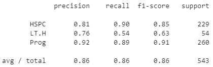
Figure 7.21 – Results of the XGBoost model

With that, we can see that we managed to achieve a precision of 0.86, much higher than some of the other models we tested. The highly optimized nature of this model allows it to be very fast and robust relative to most others.

Over the course of this section, we managed to cover quite a wide scope of classification models. We began with the simple KNN model, which attempts to predict the class of a new value relative to its closest neighbors. Next, we covered SVM models, which attempt to assign labels based on specified boundaries drawn by support vectors. We then covered both decision trees and random forests, which operate based on nodes, leaves, and splits, and then finally saw a working example of XGBoost, a highly optimized model that implements many of the features we saw in other models.

As you begin to dive into the many different models for new datasets, you will likely investigate the idea of automating the model selection process. If you think about it, each of the steps we have taken above could be automated in one way or another to identify which model operates the best under a specific set of metric requirements. Luckily for us, a library already exists that can assist us in this space. Over the course of the following tutorial, we will investigate the use of these models alongside some automated machine learning capabilities on Google Cloud Platform (GCP).

Tutorial: Classification of proteins using GCP

During this tutorial, we will investigate a number of classification models, followed by an implementation of some automated machine learning capabilities. Our main objective will be to automatically develop a model for the classification of proteins using a dataset from the Research Collaboratory for Structural Bioinformatics (RCSB) Protein Data Bank (PDB). If you recall, we used data from RCSB PDB in a previous chapter to plot a 3D protein structure. The dataset we will be working with in this chapter consists of two parts—a structured dataset with rows columns, one column of which is the designated classification of each of the proteins, and a series of RNA sequences for each of the proteins. We will save this second set of sequence-based data for analysis in a later chapter and focus on the structured dataset for now.

In this chapter, we will use this structured dataset containing many different types of proteins in an attempt to develop a classifier. Given the large nature of this dataset, we will take this opportunity to move our development environment from our local installation of Jupyter Notebook to an online notebook in GCP. Before we can do so, we will need to create a new GCP account. Let's go ahead and get started.

Getting started in GCP

Getting started in GCP is quite simple, and can be accomplished in a few simple steps:

1. We can begin by navigating to https://cloud.google.com/ and registering for a new account. You will need to provide a few details, such as your name, email, and a few other items.
2. Once registered, you will be able to navigate to the console by clicking the Console button on the upper right-hand side of the page:
   

   Figure 7.22 – A screenshot of the Console button

3. Within the console page, you will be able to see all items relating to your current project, such as general information, resources used, API usage, and even billing:
   

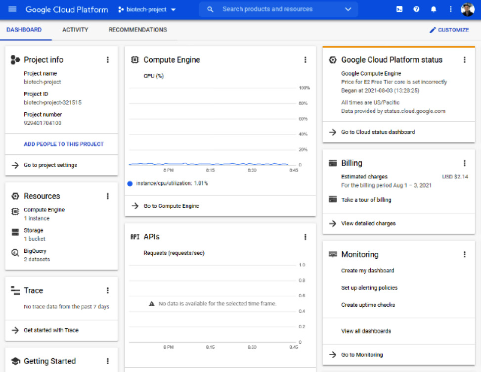
   Figure 7.23 – An example of the console page

4. You will likely not have any projects set up yet. In order to create a new project, navigate to the drop-down menu on the upper left-hand side and select the New Project option. Give your project a name and then click CREATE. You can navigate between different projects using that same drop-down menu:

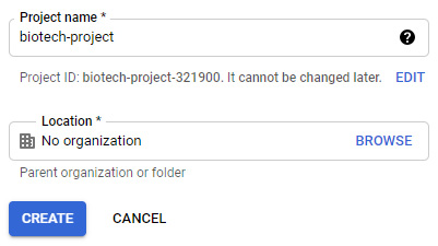
Figure 7.24 – A screenshot of the project name and location pane in GCP

With that last step completed, you are now all set up to take full advantage of the GCP platform. We will cover a few of the GCP capabilities in this tutorial to get us started in the data science space; however, I highly encourage new users to explore and learn the many tools and resources available here.

Uploading data to GCP BigQuery

There are many different ways in which you can upload data within GCP; however, we will focus on one particular capability unique to the GCP, known as BigQuery. The main idea behind BigQuery is that it is a serverless data warehouse with built-in machine learning capabilities that supports the use of queries with the SQL language. If you recall, we previously developed and deployed an AWS RDS to manage our data using an EC2 instance as a server, whereas BigQuery, on the other hand, operates using a serverless architecture. We can set up BigQuery and start uploading our data in a few simple steps:

1. Using the navigation menu on the left-hand side of the page, scroll down to the Products section, hover over the BigQuery option, and select SQL workspace. Given that this is the first time you are using this tool, you may need to activate the API. This will be true for all tools that you have never used before:
   

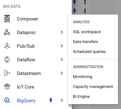
   Figure 7.25 – A screenshot of the BigQuery menu in GCP

2. Within this list, you will find the project that you created in the previous section. Click on the options button to the right and select Create dataset. In this menu, give the dataset a name, such as protein_structure_sequence, leaving all the other options as their default values. You can then click Create dataset.
3. On the left-hand menu, you will see the newly created dataset listed under the project name. If you click Options followed by Open, you will be directed to the dataset's main page. Within this page, you will find information relating to that particular dataset. Let's now go ahead and create a new table here by clicking the Create Table option at the top. Change the source to reflect the upload option and navigate to the CSV file pertaining to the protein classifications from RCSB PDB. Give the table a new name, and while leaving all other options as their default values, click Create Table:
   

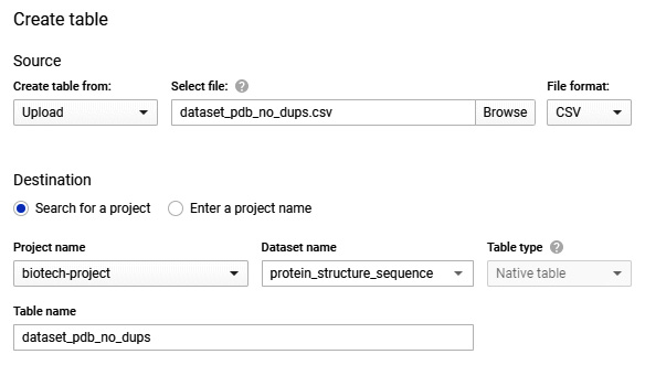
   Figure 7.26 – A screenshot of the Create table pane in GCP

4. If you navigate back to Explorer, you will see the newly created table listed under the dataset, which is listed under your project:

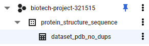
Figure 7.27 – An example of the table created within a dataset

If you managed to follow all of these steps correctly, you should now have data available for you to use in BigQuery. In the following section, we will prepare a new notebook and start parsing some of our data in this dataset.

Creating a notebook in GCP

In this section, we will create a notebook equivalent to that of the Jupyter notebooks we have been using to carry out our data science work on. We can get a new notebook set up in a few simple steps:

1. In the navigation pane on the left-hand side of the screen, scroll down to the ARTIFICIAL INTELLIGENCE section, hover over AI Platform, and select the Notebooks option. Remember that you may need to activate this API once again if you have not done so already:
   

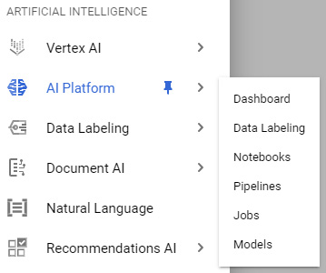
   Figure 7.28 – A visual of the AI Platform menu

2. Next, navigate to the top of the screen and select the New Instance option. There are many different options available for you depending on your needs. For the purposes of this tutorial, we can select the first option for Python 3:
   

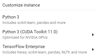
   Figure 7.29 – A screenshot of the instance options

   If you are familiar with notebook instances and are comfortable customizing them, I recommend creating a customized instance to suit your exact needs.

3. Once the notebook is created and the instance is online, you will be able to see it in the main Notebook Instances section. Go ahead and click on the OPEN JUPYTERLAB button. A new window will open up containing Jupyter Lab:
   

   Figure 7.30 – A screenshot of the instance menu

4. In the home directory, create a new directory called biotech-machine-learning for us to save our notebooks in. Open the directory and create a new notebook by clicking the Python 3 notebook option on the right:

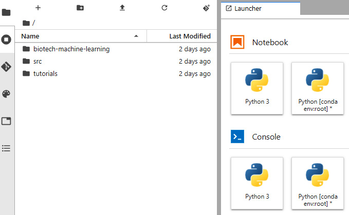
Figure 7.31 – A screenshot of Jupyter Lab on GCP

With the instance now provisioned and the notebook created, you are now all set to run all of your data science models on GCP. Let's now take a closer look at the data and begin training a few machine learning models.

Using auto-sklearn in GCP Notebooks

If you open your newly created notebook, you see the very familiar environment of Jupyter Lab that we have been working with all along. The two main benefits here are that we now have the ability to manage our datasets within this same environment and can provision larger resources to process our data relative to the few CPUs and GPUs we have on our local machines.

Recall that our main objective for getting to this state is to be able to develop a classification model to correctly classify proteins based on some input features. The dataset we are working with is known as a real-world dataset in the sense that it is not well organized, has missing values, may contain too much data, and will need some preprocessing prior to the development of any model.

Let's go ahead and start by importing a few necessary libraries:

import pandas as pd

import numpy as np

from google.cloud import bigquery

import missingno as msno

from sklearn.metrics import classification_report

import ast

import autosklearn.classification

Next, let's now import our dataset from BigQuery. We can do that directly here in the notebook by instantiating a client using the BigQuery class of the Google Cloud library:

client = bigquery.Client(location="US")

print("Client creating using default project: {}".format(client.project))

Next, we can go ahead and query our data using a SELECT command in the SQL language. We can simply begin by querying all the data in our dataset. In the following code snippet, we will query the data using SQL, and convert the results to a dataframe:

query = """

    SELECT *

    FROM `biotech-project-321515.protein_structure_sequence.dataset_pdb_no_dups`

"""

query_job = client.query(

    query,

    location="US",

)

df = query_job.to_dataframe()

print(df.shape)

Once converted to a more manageable dataframe, we can see that the dataset we are working with is quite extensive, with nearly 140,000 rows and 14 columns of data. Immediately, we notice that one of the columns is called classification. Let's take a look at the unique number of classes in this dataset using the n_unique() function:

df.classification.nunique()

We notice that there are 5,050 different classes! That is a lot for a dataset this size, indicating that we may need to reduce this quite heavily before any analysis. Before proceeding any further, let's go ahead and drop any and all potential duplicates:

dfx = df.drop_duplicates(["structureId"])

Let's now take a closer look at the top 10 classes in our dataset by count:

dfx.classification.value_counts()[:10].sort_values().plot(kind = 'barh')

The following figure is yielded from the code, showing us the top 10 classes from this dataset:

Figure 7.32 – The top 10 most frequent labels in the dataset

Immediately, we notice that there are two or three classes or proteins that account for the vast majority of this data: hydrolase, transferase, and oxidoreductase. This will be problematic for two reasons:

• Data should always be balanced in the sense that each of the classes should have a roughly equal number of rows.
• As a general rule of thumb, the ratio of classes to observations should be around 50:1, meaning that with 5,050 classes, we would require around 252,500 observations, which we do not currently have.

Given these two constraints, we can account for both by simply focusing on developing a model using the first three classes. For now, we notice that there are quite a few features available to us regardless of the classes at hand. We can go ahead and take a closer look at the completeness of our features of interest using the msno library:

dfx = dfx[["classification", "residueCount", "resolution", "resolution", "crystallizationTempK", "densityMatthews", "densityPercentSol", "phValue"]]

msno.matrix(dfx)

The following screenshot, representing the completeness of the dataset, is then generated. Notice that a substantial number of rows for the crystallizationTempK feature are missing:

Figure 7.33 – A graphical representation showing the completeness of the dataset

So far within this dataset, we have noted the fact that we will need to reduce the number of classes to the top two classes to avoid an imbalanced dataset, and we will also need to address the many rows of data we are missing. Let's go ahead and prepare our dataset for the development of a few classification models based on our observations. First, we can go ahead and reduce the dataset using a simple groupby function:

df2 = dfx.groupby("classification").filter(lambda x: len(x) > 14000)

df2.classification.value_counts()

If we run a quick check on the dataframe using the value_counts() function, we notice that we were able to reduce it down to the top two labels.

Alternatively, we can run this same command in SQL using a few clever joins. We can begin with our inner query in which we SELECT the classification and COUNT the residueCount feature and the GROUP BY classification. Next, we INNER JOIN that query with the original table setting, classification against classification, but filtering using our WHERE clause:

query = """

    SELECT DISTINCT

        dups.*

    FROM (

        SELECT classification, count(residueCount) AS classCount

        FROM `biotech-project-321515.protein_structure_sequence.dataset_pdb_no_dups`

        GROUP BY classification

    ) AS sub

    INNER JOIN `biotech-project-321515.protein_structure_sequence.dataset_pdb_no_dups` AS dups

        ON sub.classification = dups.classification

    WHERE sub.classCount > 14000

"""

query_job = client.query(

    query,

    location="US",

)

df2 = query_job.to_dataframe()

Next, we can go ahead and remove the rows of data with missing values using the dropna() function:

df2 = df2.dropna()

df2.shape

Immediately, we observe that the size of the dataset has been reduced down to 24,179 observations. This will be a sufficient dataset to work with when developing our models. In order to avoid having to process it again, we can write the contents of the dataframe to a new table in the same BigQuery dataset:

import pandas_gbq

pandas_gbq.to_gbq(df2, 'protein_structure_sequence.dataset_pdb_no_dups_cleaned', project_id ='biotech-project-321515', if_exists='replace')

With the data now prepared, let's go ahead and develop a model. We can go ahead and split the input and output data, scale the data using the StandardScaler class, and split the data into test and training sets:

X = df2.drop(columns=["classification"])

y = df2.classification.values.ravel()

from sklearn.preprocessing import StandardScaler

scaler = StandardScaler()

X_scaled = scaler.fit_transform(X)

from sklearn.model_selection import train_test_split

X_train, X_test, y_train, y_test = train_test_split(X_scaled, y, test_size=0.25)

For the automation section, we will use a library called autosklearn, which can be installed using the command line via pip:

pip install autosklearn

With the library installed, we can go ahead and import the library and instantiate a new instance of that model. We will then set a few parameters relating to the time we wish to dedicate to this process and give the model a temporary directory to operate in:

import autosklearn.classification

automl = autosklearn.classification.AutoSklearnClassifier(

    time_left_for_this_task=120,

    per_run_time_limit=30,

    tmp_folder='/tmp/autosklearn_protein_tmp5',

)

Finally, we can go ahead and fit the model on our data. This process will take a few minutes to run:

automl.fit(X_train, y_train, dataset_name='dataset_pdb_no_dups')

When the model is complete, we can take a look at the results by printing the leader board:

print(automl.leaderboard())

Upon printing the leaderboard, we retrieve the following results:

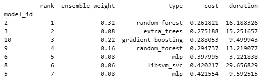
Figure 7.34 – Results of the auto-sklearn model

We can also take a look at the top-performing random_forest model using the get_models_with_weights() function:

automl.get_models_with_weights()[0]

We can also go ahead and get a few more metrics by making some predictions using the model and the classification_report() function:

predictions = automl.predict(X_test)

print("classification_report:", classification_report(y_test, predictions))

Upon printing the report, this yields the following results:

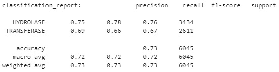
Figure 7. 35 – Results of the top-performing auto-sklearn model

With that, we managed to develop a machine learning model successfully and automatically for our dataset. However, the model has not yet been fined-tuned or optimized for this task. One challenge that I recommend you complete is the process of tuning the various parameters in this model in an attempt to increase our metrics. In addition, another challenge would be to try and explore some of the other models we learned about and see whether any of them can beat autosklearn. Hint: XGBoost has always been a great model for structured datasets.

Using the AutoML application in GCP

In the previous section, we used an open source library called auto-sklearn that automates the process in which models can be selected using the sklearn library. However, as we have seen with the XGBoost library, there are many other models out there outside of the sklearn API. GCP offers a robust tool, similar to that of auto-sklearn, that iterates over a large selection of models and methods to find the most optimal model for a given dataset. Let's go ahead and give this a try:

1. In the navigation menu in GCP, scroll down to the ARTIFICIAL INTELLIGENCE section, hover over Tables, and select Datasets:
   

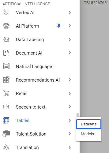
   Figure 7.36 – Selecting Datasets from the ARTIFICIAL INTELLIGENCE menu

2. At the top of the page, select the New Dataset option. At the time this book was written, the beta implementation of the model was available. Some of the steps will likely have changed in future implementations:
   

   Figure 7.37 – A screenshot of the button to create a new dataset

3. Go ahead and give the dataset a name and region and click Create Dataset.
4. We have the option to import our dataset of interest either as a raw CSV file or using BigQuery. Go ahead and import our cleaned version of the proteins dataset by specifying projectID, datasetID, and the table name, and then click Import.
5. In the TRAIN section, you will have the ability to see the tables within this dataset. Go ahead and specify the Classification column as the target column and then click TRAIN MODEL:
   

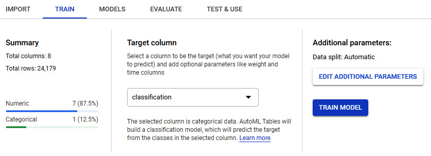
   Figure 7.38 – An example of the training menu

6. The model selection process will take some time to complete. Upon completion, you will be able to see the results of the model under the Evaluate tab. Here you will get a sense of the classification metrics we have been working with, as well as a few others.

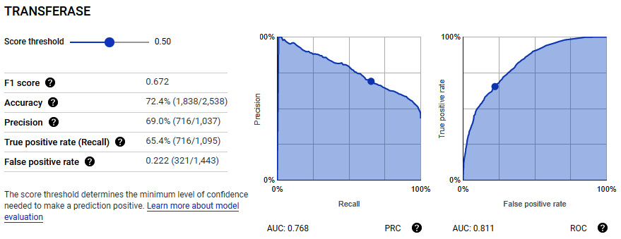
Figure 7.39 – Results of the trained model showing the metrics

GCP AutoML is a powerful tool that you can use to your advantage when handling a difficult dataset. You will find that the implementation of the model is quite robust and generally comprehensive relative to the many options that we, as data scientists, can explore. One of the downsides of AutoML is the fact that the final model is not shared with the user; however, the user does have the ability to test new data and use the model later on. We will explore another option similar to AutoML in the following section known as AutoPilot in AWS. Now that we have explored quite a few different models and methods relating to classification, let's go and explore their respective counterparts when it comes to regression.

Understanding regression in supervised machine learning

Regressions are models generally used to determine the relationship or correlation between dependent and independent variables. Within the context of machine learning, we define regressions as supervised machine learning models that allow for the identification of correlations between two or more variables in order to generalize or learn from historical data to make predictions on new observations.

Within the confines of the biotechnology space, we use regression models to predict values in many different areas.

• Predicting the LCAP of a compound ahead of time
• Predicting titer results further upstream
• Predicting the isoelectric point of a monoclonal antibody
• Predicting the decomposition percentages of compounds

Correlations are generally established between two columns. Two columns within a dataset are said to have a strong correlation when a dependence is observed. The specific relationship can be better understood using a linear regression model such that:

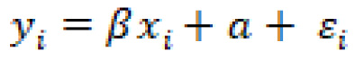
In which is the first feature, is the second feature, is a small error term, with and as constants. Using this simple equation, we can understand our data more effectively, and calculate any correlation. For example, recall earlier we observed a correlation in the toxicity dataset, specifically between the MolWt and HeavyAtoms features.

The main idea behind any given regression model, unlike its classification counterparts, is to output a continuous value rather than a class or category. For example, we could use a number of columns in the toxicity dataset in an attempt to predict other columns in the same dataset.

There are many different types of regression models commonly used in the data science space. There are linear regressions that focus on optimizing a linear relationship between a set of variables, logistic regression that acts more as a binary classifier rather than regressors, and ensemble models that combine the predictive power of several base estimators, among many others. We can see some examples in Figure 7.40:

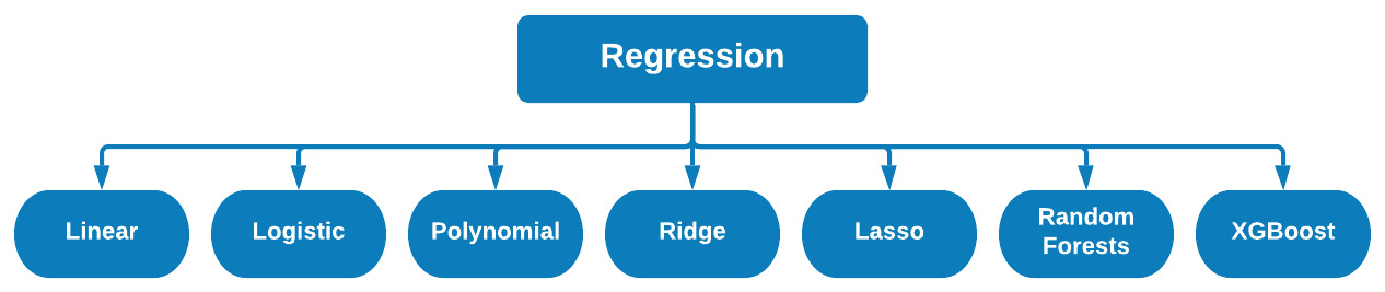
Figure 7.40 – Different types of regression models

Over the course of this section, we will explore a few of these models as we investigate the application of a few regression models using the toxicity dataset. Let's go ahead and prepare our data.

We can begin by importing our libraries of interest:

import pandas as pd

import numpy as np

from sklearn.metrics import r2_score

from sklearn.metrics import mean_squared_error

import matplotlib.pyplot as plt

import seaborn as sns

sns.set_theme(color_codes=True)

Next, we can go ahead and import our dataset and drop the missing rows. For practice, I suggest you upload this dataset to BigQuery, just as we did in the previous section, and query your data using SQL via a SELECT statement:

df = pd.read_csv("../../datasets/dataset_toxicity_sd.csv")

df = df.dropna()

Next, we can split our data into input and output values, and scale our data using the MinMaxScaler() class from sklearn:

X = df[["Heteroatoms", "MolWt", "HeavyAtoms", "NHOH", "HAcceptors", "HDonors"]]

y = df.TPSA.values.ravel()

from sklearn.preprocessing import MinMaxScaler

scaler = MinMaxScaler()

X_scaled = scaler.fit_transform(X)

Finally, we can split the dataset into training and test data:

from sklearn.model_selection import train_test_split

X_train, X_test, y_train, y_test = train_test_split(X_scaled, y, test_size=0.25)

With our dataset prepared, we are now ready to go ahead and start exploring a few regression models.

Exploring different regression models

There are many types of regression methods that can be used with a given dataset. We can think of regression as falling into four main categories: linear regressions, logistic regressions, ensemble regressions, and finally, boosted regressions. Throughout the next section, we will be exploring examples from each of these categories, starting with linear regression.

Single and multiple linear regression

In many of the datasets you will likely encounter in your career, you oftentimes find that some of the features exhibit some type of correlation vis-à-vis one another. Earlier in this chapter, we discussed the idea of a correlation between two features as a dependence of one feature upon another, which can be calculated using the Pearson correlation metric known as R2. Over the last few chapters, we have looked at the idea of correlations in a few different ways, including heats maps and pairplots.

Using the dataset we just prepared, we can take a look at a few correlations using seaborn:

import seaborn as sns

fig = sns.pairplot(data=df[["Heteroatoms", "MolWt", "HeavyAtoms"]])

This yields the following figure:

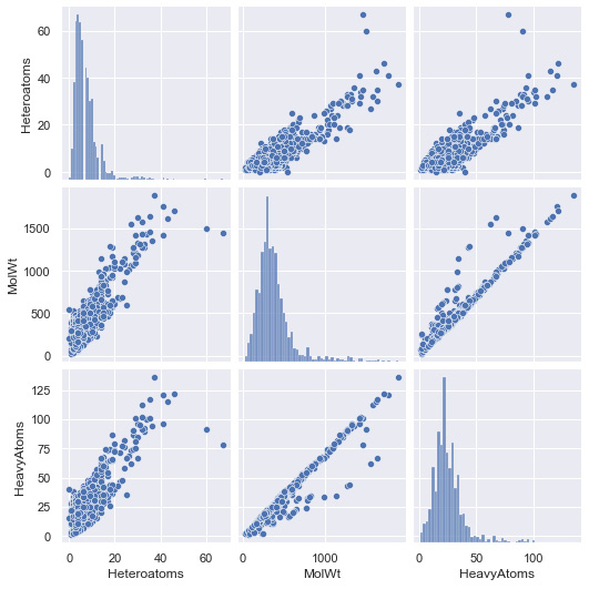
Figure 7.41 – Results of the pairplot function using the toxicity dataset

We can see that there are a few correlations in our dataset already. Using simple linear regression, we can take advantage of this correlation in the sense that we can use one variable to predict what the other will most likely be. For example, if X was the independent variable, and Y was the dependent variable, we can define the linear relationship between the two as:

In which m is the slope and c is the y intercept. This equation should be familiar to you based on some of the earlier content in this book, as well as your math classes in high school. Using this relationship, our objective will be to optimize this line relative to our data in order to determine the values for m and c using a method known as the least squares method.

Before we can discuss the least squares method, let's first discuss the idea of a loss function. A loss function within the context of machine learning is a measure of the difference between our calculated and expected values. For example, let's examine the quadratic loss function, commonly used to calculate loss within a regression model, which we can define as:

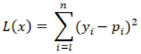
By now, I would hope you recognize this function from our discussions in the Measuring success section. Can you tell me where we last used this?

Now that we have discussed the idea of loss functions, let's take a closer look at the least squares method. The main idea behind this mathematical method is to determine a line of best fit for a given set of data, as demonstrated by the correlations we just saw, by minimizing the loss. To fully explain the concepts behind this equation we would need to discuss partial derivatives and what not. For the purposes of simplicity, we will simply define the least squares method as a process for minimizing loss in order to determine a line of best fit for a given dataset.

We can divide linear regressions into two main categories: simple linear regression and multiple linear regression. The main idea here concerns the number of features we will be training the model with. If we are simply training the model based on one feature, we will be developing a simple linear regression. On the other hand, if we train the model using multiple features, we would be training a multiple regression model.

Whether you are training a simple or multiple regression model, the process and desired outcomes are generally the same. Ideally, the output of our models when plotted against the actual values should result in a linear line showing a strong correlation in our data, as depicted in Figure 7.42:

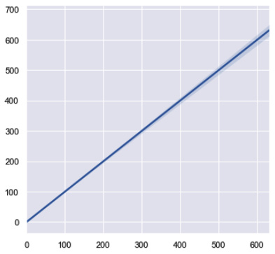
Figure 7.42 – A simple linear line showing the ideal correlation

Let's go ahead and explore the development of a multiple linear regression model. With the data imported in the previous section, we can import the LinearRegression class for sklearn, fit it with our training data, and make a prediction using the test dataset:

from sklearn.linear_model import LinearRegression

reg = LinearRegression().fit(X_train, y_train)

y_pred = reg.predict(X_test)

Next, we can go ahead and use the actual and predicted values to both calculate the R2 value and visualize on the graph. In addition, we will also capture the MSE metric:

p = sns.jointplot(x=y_test, y=y_pred, kind="reg")

p.fig.suptitle(f"Linear Regression, R2 = {round(r2_score(y_test, y_pred), 3)}, MSE = {round(mean_squared_error(y_test, y_pred), 2)}")

p.fig.subplots_adjust(top=0.90)

The code will then yield the following figure:

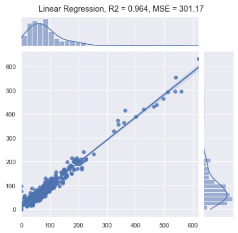
Figure 7.43 – Results of the linear regression model

Immediately, we notice that this simple linear regression model was quite effective in making predictions on our dataset. Notice that this model not only used one feature, but used all of the features to make its prediction. We notice from the graph that the vast majority of our data is localized at the bottom left. This is not ideal for a regression model as we would prefer the values to be equally dispersed across all bounds; however, it is important to remember that in the biotechnology space, you will almost always encounter real-world data in which you will observe items such as these.

If you are following along in Jupyter Notebooks, go ahead and reduce the dataset to only one input feature, scale and split the data, train a simple linear regression, and compare the results to the multiple linear regression. Does the correlation of our predictions and actual values increase or decrease?

Logistic regression

Recall that in the linear regression section, we discussed the methodology in which a single linear line can be used to predict a value based on a correlated feature as input. We outlined the linear equation as follows:

In some instances, the relationship between the data and the desired output may not be best represented by a linear model, but rather a non-linear one:

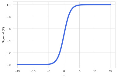
Figure 7.44 – A simple sigmoid curve

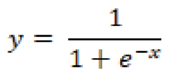
Although known as logistic regression, this regression is mostly used as a binary classification algorithm. However, the main focus here is that the word logistic is referring to the logistic function, also known as the Sigmoid function, represented as:

With this in mind, we will want to use this function to make predictions in our dataset. If we wanted to determine whether or not a compound was toxic given a specific input value, we could calculate the weighted sum of inputs such that:

This would allow us to calculate the probability of toxicity such that:

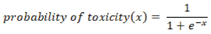
Using this probability, a final prediction can be made, and an output value assigned. Go ahead and implement this model using the protein classification dataset in the previous section and compare the results that you find to those of the other classifiers.

Decision trees and random forest regression

Similar to its classification counterpart, Decision Tree Regressions (DTRs) are commonly used machine learning models implementing nearly the same internal mechanisms that decision tree classifiers use. The only difference between the models is the fact that regressors output continuous numerical values, whereas classifiers output discrete classes.

Similarly, another model known as Random Forest Regressors (RFRs) also exists and operates similarly to its classification counterparts. This model is also an ensemble method in which each tree is trained as a separate model and subsequently averaged.

Let's go ahead and implement an RFR using this dataset. Just as we have previously done, we will first create an instance of the model, fit it to our data, make a prediction, and visualize the results:

from sklearn.ensemble import RandomForestRegressor

reg = RandomForestRegressor().fit(X_train, y_train)

y_pred = reg.predict(X_test)

p = sns.jointplot(x=y_test, y=y_pred, kind="reg")

p.fig.suptitle(f"RandomForestRegressor Regression, R2 = {round(r2_score(y_test, y_pred), 3)}, MSE = {round(mean_squared_error(y_test, y_pred), 2)}")

# p.ax_joint.collections[0].set_alpha(0)

# p.fig.tight_layout()

p.fig.subplots_adjust(top=0.90)

With the model developed, we can visualize the results using the following plot:

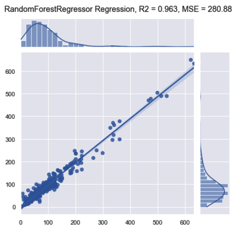
Figure 7.45 – Results of the random forest regression model

Notice that while the R2 remained relatively the same, the MSE did decrease substantially relative to the first linear model. We can improve these scores by tuning the model's parameters. We can demonstrate this using the max_depth parameter:

for i in range(1,10):

    reg = RandomForestRegressor(max_depth=i)

                       .fit(X_train, y_train)

    y_pred = reg.predict(X_test)

    print("depth =", i,

          "score=", r2_score(y_test, y_pred),

          "mse = ", mean_squared_error(y_test, y_pred))

The output for this code is shown below, indicating that a max_depth of 8 would likely be optimal given that it results in an R2 of 0.967 and an MSE of 248.133:

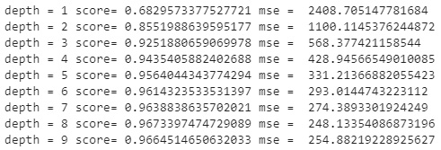
Figure 7.46 – Results of the random forest regression model with differing max_depth

Similar to classification, decision trees for regression tend to be excellent methods for allowing you to develop models while trying to avoid overfitting your data. Another great benefit of DTR models, when using the sklearn API, is gaining insights into feature importance directly from the model. Let's go ahead and demonstrate this:

features = X.columns

importances = reg.feature_importances_

indices = np.argsort(importances)[-9:]

plt.title('Feature Importances')

plt.barh(range(len(indices)), importances[indices],  

                           color='royalblue',

                           align='center')

plt.yticks(range(len(indices)),[features[i] for i in indices])

plt.xlabel('Relative Importance')

plt.show()

With that complete, this yields the following diagram:

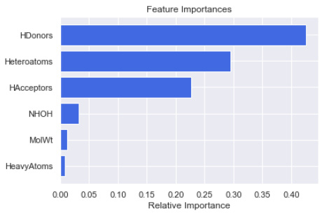
Figure 7.47 – Feature importance of the random forest regression model

Looking at this figure, we can see that the top three features that had the biggest impact on the development of this model were HDonors, Heteroatoms, and HAcceptors. Although this example of feature importance was developed using the RFR model, we can theoretically use this with many other models. One library in particular that has gained a great deal of importance in the field concerning the idea of feature importance is the SHAP library. It is highly recommended that you take a glance at this library and the many wonderful features (no pun intended) that it has to offer.

XGBoost regression

Similar to the XGBoost classification model we investigated in the previous section, we also have regression implementation, which allows us to predict a value rather than a category. We can go ahead and implement this easily, just as we did in the previous section:

import xgboost as xg

reg = xg.XGBRegressor(objective ='reg:linear',n_estimators = 1000).fit(X_train, y_train)

y_pred = reg.predict(X_test)

p = sns.jointplot(x=y_test, y=y_pred, kind="reg")

p.fig.suptitle(f"xgboost Regression, R2 = {round(r2_score(y_test, y_pred), 3)}, MSE = {round(mean_squared_error(y_test, y_pred), 2)}")

p.fig.subplots_adjust(top=0.90)

With the code completed, this yields the following figure:

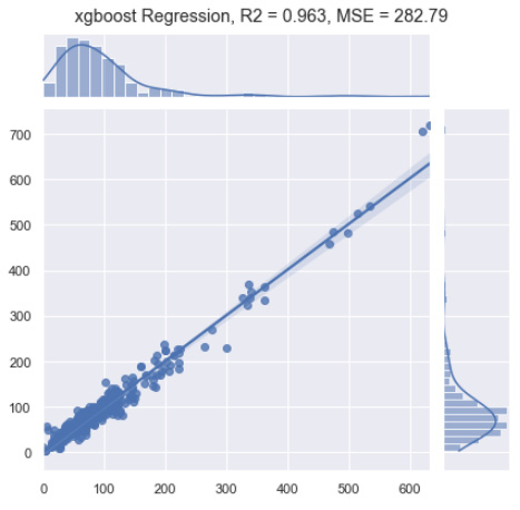
Figure 7.48 – Results of the XGBoost regression model

You will notice that this implementation of the model gave us a very respectable R2 value in the context of our actual and predicted values and managed to yield an MSE of 282.79, which is slightly less than some of the other models we've attempted in this chapter. With the model completed, let's now move on to see how we could use some of the automated machine learning functionality provided in AWS in the following tutorial.

Tutorial: Regression for property prediction

Over the course of this chapter, we have reviewed some of the most common (and popular) regression models as they relate to the prediction of the TPSA feature using the toxicity dataset. In the previous section pertaining to classification, we created a GCP instance and used the auto-sklearn library to automatically identify one of the top machine learning models for a given dataset. In this tutorial, we will create an AWS SageMaker notebook, query our dataset from RDS, and run the auto-sklearn library in a similar manner. In addition, we will also explore an even more powerful automated machine learning method using AWS Autopilot. In one of the earlier chapters, we used AWS RDS to launch a relation database to host our toxicity dataset. Using that same AWS account, we will now go ahead and get started.

Creating a SageMaker notebook in AWS

Similar to the creation of a notebook in GCP, we can create a SageMaker notebook in AWS in a few simple steps:

1. Navigate to the AWS Management Console on the front page. Click on the Services drop-down menu and select Amazon SageMaker under the Machine Learning section:
   

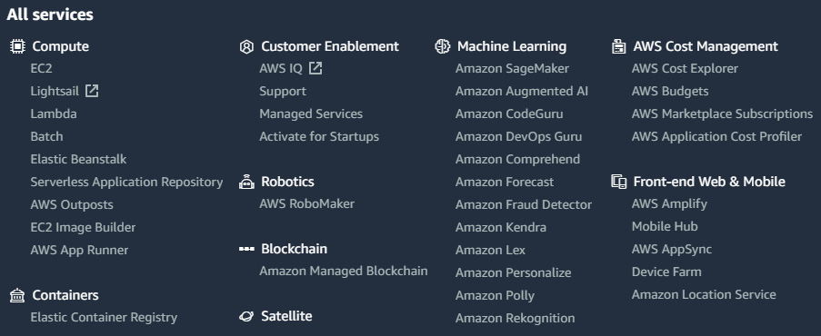
   Figure 7.49 – The list of services provided by AWS

2. On the left-hand side of the page, click the Notebook drop-down menu and then select the Notebook instances button:
   

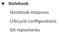
   Figure 7.50 – A screenshot of the notebook menu

3. Within the notebook instances menu, click on the orange button called Create notebook instance:
   

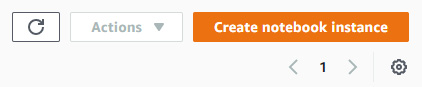
   Figure 7.51 – A screenshot of the Create notebook instance button

4. Let's now go ahead and give the notebook instance a name, such as biotech-machine-learning. We can leave the instance type as the default selection of ml.t2.medium. This is a medium-tier instance and is more than enough for the purposes of our demo today:
   

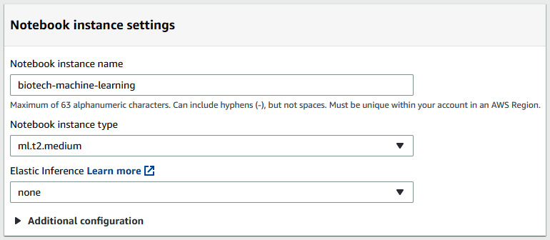
   Figure 7.52 – A screenshot of the notebook instance settings

5. Under the Permissions and encryption section, select the Create a new role option for the IAM role section. The main idea behind IAM roles is the concept of granting certain users or roles the ability to interact with specific AWS resources. For example, we could allow this role to also have access to some but not all S3 buckets. For the purposes of this tutorial, let's go ahead and grant this role access to any S3 bucket. Go ahead and click on Create role:
   

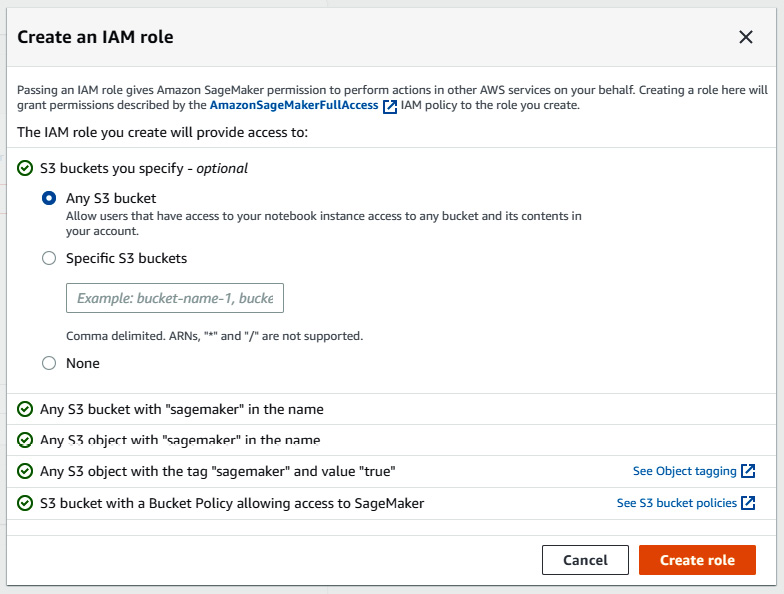
   Figure 7.53 – Creating an IAM role in AWS

6. Leaving all the other options as they are, go ahead and click on Create notebook instance. You will be redirected back to the Notebook instance menu where you will see your newly created instance in a Pending state. Within a few moments, you will notice that status change to InService. Click on the Open JupyterLab button to the right of the status:
   

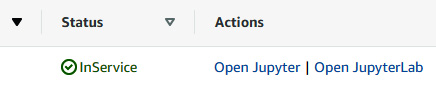
   Figure 7.54 – The options to open a Jupyter notebook or Jupyer lab in AWS

7. Once again, you will find yourself in the familiar Jupyter environment you have been working in.

   AWS SageMaker is a great resource for you to use at a very low cost. Within this space, you will be able to run all of the Python commands and libraries you have learned throughout this book. You can create directories to organize your files and scripts and access them anywhere in the world without having to have your laptop with you. In addition, you will also have access to almost 100 SageMaker sample notebooks and starter code for you to use.

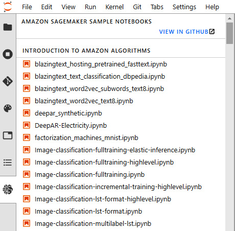
Figure 7.55 – An example list of the SageMaker starter notebooks

With this final step complete, we now have a fully working notebook instance. In the following section, we will use SageMaker to import data and start running our models.

Creating a notebook and importing data in AWS

Given that we are once again working in our familiar Jupyter space, we can easily create a notebook by selecting one of the many options on the right-hand side and start running our code. Let's go ahead and get started:

1. We can begin by selecting the conda_python3 option on the right-hand side, creating a new notebook for us in our current directory:

       

   

   Figure 7.56 – A screenshot of conda_python3

2. With the notebook prepared, we will need to install a few libraries to get started. Go ahead and install mysql-connector and pymysql using pip:

   pip install mysql-connector pymysql

3. Next, we will need to import a few things:

   import pandas as pd

   import mysql.connector

   from sqlalchemy import create_engine

   import sys

   import seaborn as sns

4. Now, we can define some of the items we will need to query our data, as we did previously in Chapter 3, Getting Started with SQL and Relational Databases:

   ENDPOINT="toxicitydataset.xxxxxx.us-east-2.rds.amazonaws.com"

   PORT="3306"

   USR="admin"

   DBNAME="toxicity_db_tutorial"

   PASSWORD = "xxxxxxxxxxxxxxxxxx"

5. Next, we can go ahead and create a connection to our RDS instance:

   db_connection_str = 'mysql+pymysql://{USR}:{PASSWORD}@{ENDPOINT}:{PORT}/{DBNAME}'.format(USR=USR, PASSWORD=PASSWORD, ENDPOINT=ENDPOINT, PORT=PORT, DBNAME=DBNAME)

   db_connection = create_engine(db_connection_str)

6. Finally, we can go ahead and query our data using a basic SQL SELECT statement:

   df = pd.read_sql('SELECT * FROM dataset_toxicity_sd', con=db_connection)

With that complete, we are now able to query our data directly from AWS RDS. As you begin to explore new models in the realm of data science, you will need a place to store and organize your data. Selecting a platform such as AWS RDS, AWS S3, or even GCP BigQuery will help you organize your data and studies.

Running auto-sklearn using the toxicity dataset

Now that we have our data in a working notebook, let's go ahead and use the auto-sklean library to identify a model best suited for our given dataset:

1. We can begin by installing the auto-sklearn library in our SageMaker instance:

   pip install auto-sklearn

2. Next, we can isolate our input features and output values and scale them accordingly:

   X = df[["Heteroatoms", "MolWt", "HeavyAtoms", "NHOH", "HAcceptors", "HDonors"]]

   y = df.TPSA.values.ravel()

   from sklearn.preprocessing import MinMaxScaler

   scaler = MinMaxScaler()

   X_scaled = scaler.fit_transform(X)

3. With the data scaled, we can now go ahead and separate our training and test datasets:

   from sklearn.model_selection import train_test_split

   X_train, X_test, y_train, y_test = train_test_split(X_scaled, y, test_size=0.25)

4. Finally, we can import the regression implementation of sklearn, adjust the parameters, and fit the model to our dataset:

   import autosklearn.regression

   automl = autosklearn.regression.AutoSklearnRegressor(

       time_left_for_this_task=120,

       per_run_time_limit=30,

       tmp_folder='/tmp/autosklearn_regression_example_tmp2')

   automl.fit(X_train, y_train, dataset_name='dataset_toxicity')

5. Once the model is done, we can take a look at the top-performing candidate model using the get_models_with_weights() function:

   automl.get_models_with_weights()[0]

6. Lastly, we can go ahead and get a sense of the model's performance using the R2 and MSE metrics, as we have done previously:

   from sklearn.metrics import r2_score, mean_squared_error

   predictions = automl.predict(X_test)

   p = sns.jointplot(x=y_test, y=predictions, kind="reg")

   p.fig.suptitle(f"automl, R2 = {round(r2_score(y_test, predictions), 3)}, MSE = {round(mean_squared_error(y_test, predictions), 2)}")

   # p.ax_joint.collections[0].set_alpha(0)

   # p.fig.tight_layout()

   p.fig.subplots_adjust(top=0.90)

   Upon plotting the output, this yields the following results:

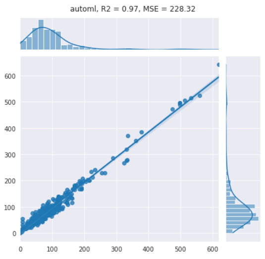
Figure 7.57 – Results of the AutoML model showing the correlation of 0.97

We can see from the figure above that the actual results and predicted results line up quite nicely, giving us an R2 value of approximately 0.97, showing a strong correlation. In the following section, we will explore the process of automating parts of the model development process using AWS Autopilot.

Automated regression using AWS Autopilot

Many different tools and applications can be found in the AWS Management Console, offering solutions to many data science and computer science problems any developer will likely encounter. There is one tool in particular that has stood out and begun to grow in popularity among the data science community known as AWS Autopilot. The purpose of AWS Autopilot is to help automate some of the tasks generally undertaken in any given data science project. We can see a visual representation of this in Figure 7.58:

Figure 7.58 – The Autopilot pipeline

Users are able to load in their datasets, identify a few parameters, and let the model take it from there as it identifies the top-performing models, optimizes a few parameters, and even generates sample code for the user to take and optimize even further. Let's go ahead and demonstrate the use of this model using the same dataset:

1. We can begin by creating a SageMaker Studio instance by navigating to the SageMaker console and selecting the Open SageMaker Studio button on the right. Using the quick start option, the default settings, and a new IAM role, click the Submit button. After a few moments, the instance will provision. Click on the Open Studio button:
   

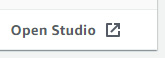
   Figure 7.59 – The Open Studio option in AWS

2. While the instance is provisioning, let's upload our dataset to S3. Using the AWS Management Console, select the S3 option under the storage section. Here, you can create buckets, which act as online storage spaces. Create a new bucket called biotech-machine-learning while keeping all the other options at their default values.
   

   Figure 7.60 – Creating a bucket in AWS

3. Once created, open the bucket and click on the Upload button. Then, upload the CSV file of the reduced and cleaned proteins dataset.
   

   Figure 7.61 – Uploading files in AWS

4. With the dataset uploaded, let's now head back to SageMaker. Using the navigation pane on the left, select the SageMaker Components and Registries tab. Using the drop-down menu, select Experiments and trials, and then click the Create Autopilot Experiment button:
   

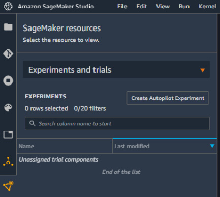
   Figure 7.62 – Creating SageMaker resources in AWS SageMaker Studio

5. Let's move on and give the experiment a name, such as dataset-pdb-nodups-cleaned.
6. In the CONNECT YOUR DATA section, select the S3 bucket name you created earlier, as well as the dataset filename:
   

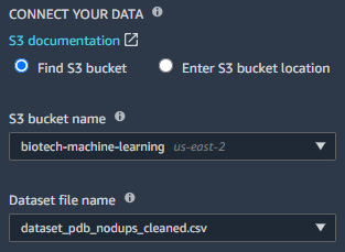
   Figure 7.63 – Connecting data to the experiment

7. Next, select the target column, which in our case, is the classification column:
   

   Figure 7.64 – Selecting a target column for the model training process

8. Finally, you can now go ahead and disable the Auto deploy option and click Create Experiment. Similar to GCP's AutoML, the application will identify a set of models deemed to be the best fit for your given dataset. You have the option to select between Pilot or Complete.

   A complete experiment will train and tune the model while allowing users to view the details and statistics in real time. It will go through various phases, such as preprocessing, candidate definition generation, feature engineering, model tuning, and report generation.

9. Upon completing the process, a dashboard with all the trained models and their associated metrics will be presented, as depicted in Figure 7.65. Users can explore the models and deploy them in a few simple clicks.

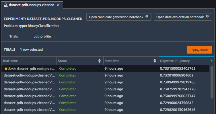
Figure 7.65 – Results of the Autopilot model

AWS Autopilot is a robust and useful tool that every data scientist can utilize when facing a difficult dataset. It not only assists in identifying the best model for a given dataset, but can also help preprocess the data, tune the model, and provide sample code for users to use.

Summary

Congratulations! We finally made it to the end of a very dense, yet very informative chapter. In this chapter, we learned quite a few different things. In the first half of this chapter, we explored the realm of classification and demonstrated the application of a number of models using the single-cell RNA dataset – a classical application in the field of biotechnology and life sciences. We learned about a number of different models, including KNNs, SVMs, decision trees, random forests, and XGBoost. We then moved our data and code to GCP, where we stored our data in BigQuery, and provisioned a notebook instance to run our code in. In addition, we learned how to automate some of the manual and labor-intensive parts of the model development process as it pertains to the protein classification dataset using auto-sklearn. Finally, we took advantage of GCP's AutoML application to develop a classification model for our dataset.

In the second half of this chapter, we explored the realm of regression as it pertains to the toxicity dataset. We explored the idea of correlation within data and learned a few important regression models too. Some of the models we looked at included simple and multiple linear regression, logistic regression, decision tree regressors, and an XGBoost regressor as well. We then moved our code to AWS's SageMaker platform and used the previously provisioned RDS to query our data and run auto-sklearn for regression as well. Finally, we implemented AWS Autopilot's automated machine learning model for the toxicity dataset.

So far, we have spent much of our time developing machine learning models using the sklearn library. However, not every dataset can be classified or regressed using machine learning – sometimes, a more powerful set of models will be needed. For datasets such as those, we can turn to the field of deep learning, which will be our focus for the next chapter.