Chapter 4: Training a Predictor with AutoML

In Chapter 3, Creating a Project and Ingesting Your Data, you learned how a raw dataset obtained from a public data source could be prepared and ingested in a suitable format for Amazon Forecast. Additionally, you created your first forecasting project (which, in the service, is called a dataset group) and populated it with three datasets. These datasets included the very time series that you want to forecast and several related time series that, intuitively, will lend some predictive power to the model you are going to train.

In this chapter, you will use these ingested datasets to train a forecasting model in Amazon Forecast; this construct is called a Predictor. Following this, you will learn how to configure the training along with the impact that each configuration can have on the training duration and the quality of the results. By the end of the chapter, you will also have a sound understanding of the evaluation dashboard.

In this chapter, we're going to cover the following main topics:

• Using your datasets to train a predictor
• How Amazon Forecast leverages automated machine learning
• Understanding the predictor evaluation dashboard
• Exporting and visualizing your predictor backtest results

Technical requirements

No hands-on experience in a language such as Python or R is necessary to follow along with the content from this chapter. However, I highly recommend that you read this chapter while connected to your own AWS account and open the Amazon Forecast console to run the different actions at your end.

To create an AWS account and log in to the Amazon Forecast console, you can refer to the Technical requirements section of Chapter 2, An Overview of Amazon Forecast.

Using your datasets to train a predictor

By the end of Chapter 3, Creating a Project and Ingesting Your Data, you had ingested three datasets in a dataset group, called london_household_energy_consumption, as follows:

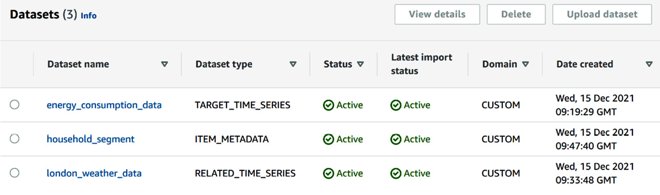
Figure 4.1 – The London household dataset group overview

From here, you are now going to train a predictor using these three datasets. To do so, from the Amazon Forecast home page, locate the View dataset groups button on the right-hand side and click on it. Then, click on the name of your project. This will display the main dashboard of your dataset group. From here, click on the Start button under the Predictor training label:

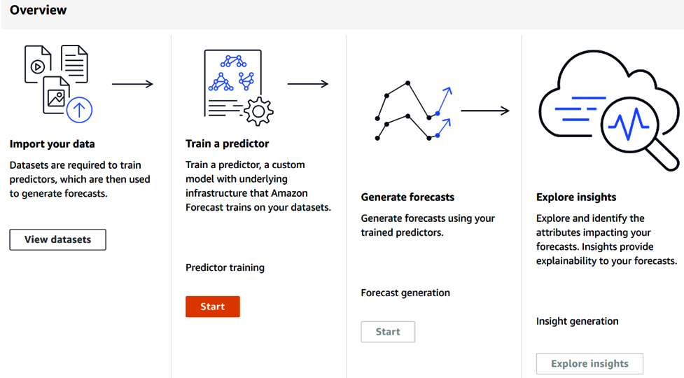
Figure 4.2 – The London household dataset group dashboard

This will bring you to the predictor configuration screen. The first two sections are dedicated to the predictor's settings: in this chapter, you are only going to modify a few of these parameters, while the other ones will be further explored in Chapter 5, Customizing Your Predictor Training:

Figure 4.3 – The basic predictor settings

You can fill in the following parameters:

• Predictor name: Let's call our predictor london_energy_automl
• Forecast frequency: We want to keep the same frequency as our original ingested data. So, let's set this parameter to 1 day.
• Forecast horizon: This is 30. As the selected forecast horizon is 1 day, this means that we want to train a model that will be able to generate the equivalent of 30 days worth of data points in the future.

You can leave the forecast dimension and forecast quantiles as their default values.

Note

It is not mandatory to have a forecast frequency that matches your dataset frequency. You can have your ingested data available hourly and then decide that you will generate a daily forecast.

In the second part of the predictor settings, you are going to disable AutoPredictor and then configure the following parameters:

• Algorithm selection: Select Choose for me (AutoML) to let Amazon Forecast choose the best algorithm given your dataset.
• Optimization metric: Select Default (by default, Amazon Forecast uses the Average wQL option. For more information regarding this, please refer to the How Amazon Forecast leverages automated machine learning section).

For reference, take a look at the following screenshot:

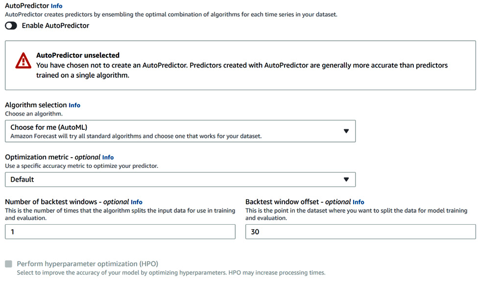
Figure 4.4 – The basic predictor settings

Leave all the other parameters with their default values, as you will explore them later in Chapter 5, Customizing Your Predictor Training.

Important Note

At the time of writing this book, the AutoPredictor option was not available. At that time, Amazon Forecast would apply a single algorithm to all the time series in your dataset. You will discover in Chapter 5, Customizing Your Predictor Training, that this might not be a good option when different segments of your dataset have significantly different behaviors.

With the AutoPredictor option, Amazon Forecast can now automatically assemble the best combination of algorithms for each time series in your dataset. In general, this creates predictors that are more accurate than single-algorithm ones, and it is now the default option when you configure a new predictor.

In addition to this, when selecting the AutoPredictor path, you can also enable Explainability to allow Amazon Forecast to provide more insights into the predictions it makes at forecast time. AutoPredictor also comes with a built-in retraining capability, which makes it easier to retrain a predictor when the underlying dataset is updated. Both the explainability feature and the retraining feature are not available for legacy predictors (predictors trained with AutoPredictor disabled).

Scroll down to the bottom of the predictor creation screen and click on the Start button. Your predictor will start training:

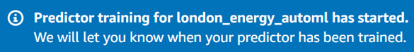
Figure 4.5 – Your first predictor starting to train

You can click on the View predictors button present on the dataset group dashboard to inspect the progress of your predictor training.

Following this, Amazon Forecast will give you the estimated time remaining and the ability to stop your training should you want to change your training parameters or cut the training cost of a predictor that is taking too long to train, as shown in the following screenshot:

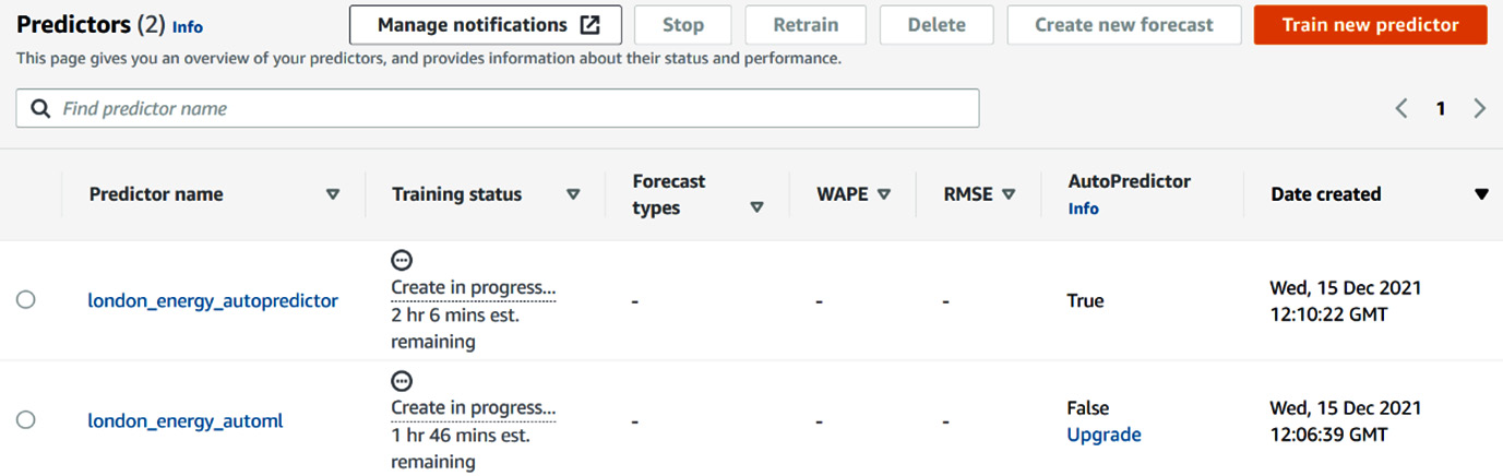
Figure 4.6 – The predictor training is in progress

Important Note

When you stop a training job, the predictor is not deleted: you can still preview its metadata. In addition, you cannot resume a stopped job.

Additionally, you have the option to upgrade a standard predictor to an AutoPredictor (as you can see in the AutoPredictor column).

Once your predictor has been trained, the Predictors list from your dataset group is updated with the key characteristics (for example, the forecast types, the WAPE metrics, and the RMSE metrics) of the trained model:

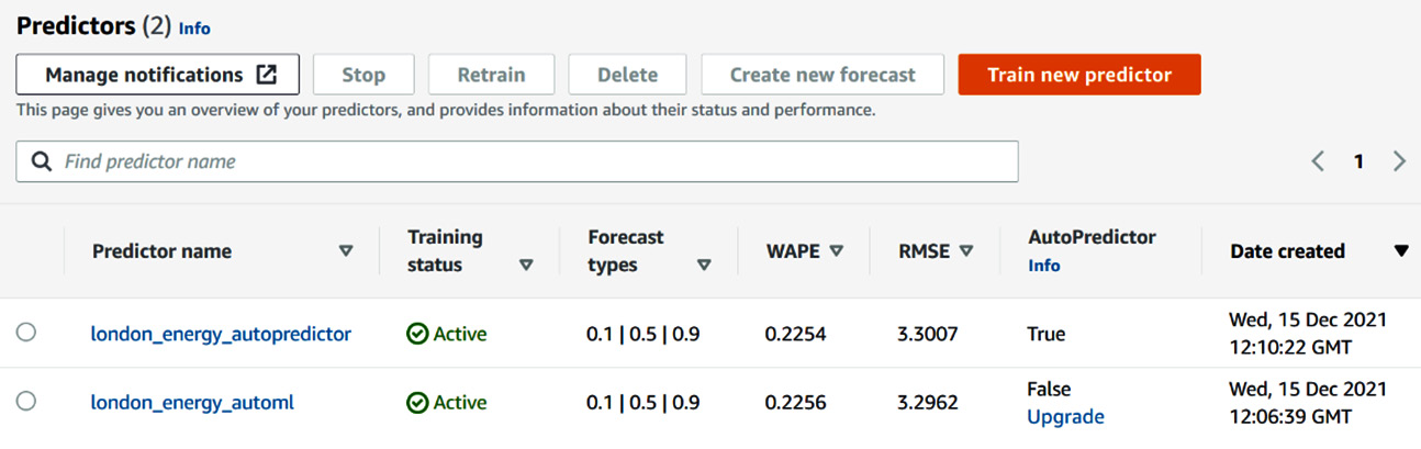
Figure 4.7 – Overview of the trained predictor

In the preceding table, you can directly access the following information:

• Training status: The trained predictors will be marked as Active.
• Forecast types: These are the different quantiles requested for your predictor. We will dive deeper into what quantiles are and when you would need to customize them in Chapter 5, Customizing Your Predictor Training. By default, Amazon Forecast will train a predictor to emit three values for each prediction point in the forecast horizon: a median value (this is also called p50 or percentile 50, which is marked here as forecast type 0.5) and an interval with a low boundary at p10 (forecast type 0.1) and a high boundary at p90 (forecast type 0.9).
• WAPE: This is one of the metrics used in forecasting to assess the quality of a prediction model. WAPE stands for Weighted Absolute Percentage Error and measures the deviation of the forecasted values from the actual values. The lower the WAPE, the better the model. Our first model, WAPE, is 0.2254.
• RMSE: This is another useful metric to assess the quality of a forecasting model. It stands for Root Mean Square Error and also measures the deviation of the forecasted values from the actual ones. The RMSE value of the model is 3.2904.
• AutoPredictor: This states whether the current predictor has been trained with AutoPredictor enabled or not, and gives you the ability to upgrade a legacy predictor to the more feature-rich AutoPredictor.

We will describe the metrics, in detail, in the Understanding the predictor evaluation dashboard section.

How Amazon Forecast leverages automated machine learning

During the training of your first predictor, you disabled AutoPredictor and then allowed the algorithm to choose its default value, which is AutoML. In Automated Machine Learning (AutoML) mode, you don't have to understand which algorithm and configuration to choose from, as Amazon Forecast will run your data against all of the available algorithms (at the time of writing, there are six) and choose the best one.

So, how does Amazon Forecast rank the different algorithms? It computes the weighted quantile loss (wQL; to read more about wQL, please check the Algorithm metrics section) for the forecast types you selected. By default, the selected forecast types are the median (p10) and the boundaries of the 80% confidence interval (p10 and p90). Amazon Forecast computes the wQL for these three quantiles. To determine the winning algorithm, it then takes the average over all of the wQL values that have been calculated: the algorithm with the lowest value will be the winning one.

My predictor obtained the following results for each algorithm:

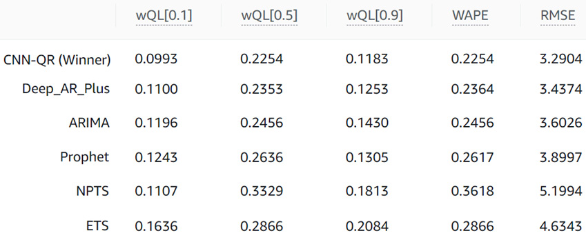
Figure 4.8 – Algorithm metrics comparison

The CNN-QR algorithm is the winner with an average wQL value of 0.1477. This value is obtained by taking the average of the wQL values for the three quantiles selected:

(wQL[0.1] + wQL[0.5] + wQL[0.9]) / 3 =

(0.0993 + 0.2254 + 0.1183) / 3 = 0.1477

Note that these metrics are computed for each backtest window. For our first training session, we set the default value to one backtest window. If you select more backtest windows (Amazon Forecast allows you to specify up to five), AutoML will average these metrics across all of them before selecting the winning algorithm.

Important Note

When running each algorithm in AutoML, Amazon Forecast uses the default parameters of each algorithm. You will see in Chapter 5, Customizing Your Predictor Training, that you can customize some of the algorithms by adjusting their hyperparameters when they are available. AutoML does not give you this option. You will have to choose between the automatic model selection (with AutoML) or hyperparameter optimization of a given algorithm that you manually select.

Understanding the predictor evaluation dashboard

When you click on a predictor name on the list of trained models that are available for your dataset group, you get access to a detailed overview screen where you can get a better understanding of the quality of your model. This screen also serves as a reminder of how your training was configured. In this section, we are going to take a detailed look at the different sections of this screen, including the following:

• Predictor overview
• Predictor metrics
• Predictor backtest results

Predictor overview

The Predictor overview section is the first section of the predictor details page:

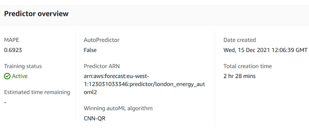
Figure 4.9 – The results page: Predictor overview

You can find three types of information in this section:

• Training parameters: These remind you how the predictor was trained. For instance, you can check whether AutoPredictor was set to True or False when training this particular predictor.
• Training results:

a) MAPE: The Mean Absolute Percentage Error (MAPE) is one of the performance metrics of a forecasting model (in our case, the MAPE value is 0.6923).

Important Note

To train a predictor, Amazon Forecast will provision and use the resources deemed necessary to deliver the results in a reasonable amount of time. During this training time, multiple compute instances might be used in parallel: the training time will be multiplied by this number of instances to compute the total cost of your training.

b) Winning AutoML algorithm: If AutoML is set to True, this field will tell you which of the underlying algorithms fared better. CNN-QR is one of the six algorithms that you will learn about, in detail, in Chapter 5, Customizing Your Predictor Training.

• Predictor attributes:
  • Predictor ARN: This is useful when you use the API and want to precisely point to a particular predictor. This is a unique identifier (ARN stands for Amazon Resource Number).
  • Date created: This is the date at which you created the predictor and started the training process.
  • Total creation time: Training my predictor took 2 hr 28 mins. This will be the training time used to compute my bills at the end of the billing cycle.

The Estimated time remaining field is only populated while the predictor is in progress. Once a predictor is active, this field becomes empty.

Predictor metrics

The next section of interest on the predictor page is the Predictor metrics one. This section shows the predictor metrics for each backtest window and each algorithm. When the predictor is trained with AutoML on, the sections open with the winning algorithm results by default (in our case, CNN-QR):

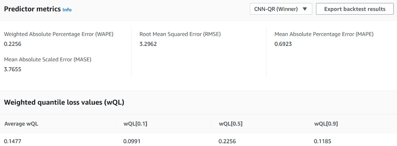
Figure 4.10 – The results page: algorithm metrics

Using the drop-down menu in the upper-right corner of this section, you can select the algorithm that you want to see the results for. As demonstrated earlier, our predictor obtained the following results for each algorithm:

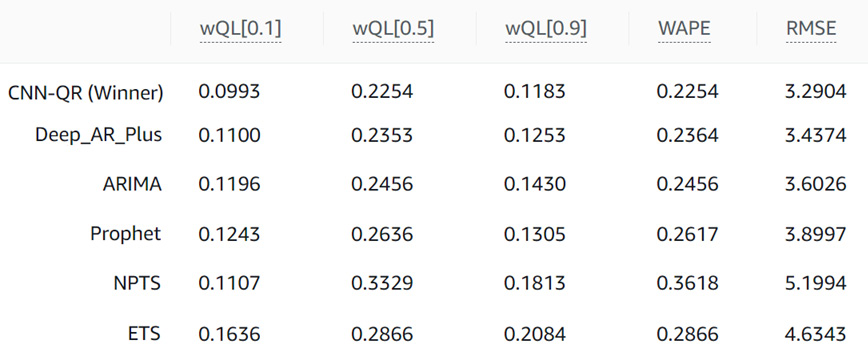
Figure 4.11 – Comparing algorithm metrics

When AutoML is enabled, Amazon Forecast selects the algorithm that delivers the best average wQL value across every forecast type (these are 0.1, 0.5, and 0.9 when you use the default quantiles). In the preceding table, CNN-QR has an average wQL value of the following:

(0.0993 + 0.2254 + 0.1183) / 3 = 0.1477

The second-best algorithm is Deep_AR_Plus with an average wQL value of the following:

(0.1100 + 0.2353 + 0.1253) / 3 = 0.1569

So, how are these metrics computed? How do you interpret them? How do you know if a value is a good one? To know more about the metrics in detail, please head over to Chapter 7, Improving and Scaling Your Forecast Strategy. You will find a dedicated section that will detail the ins and outs of these metrics and how to use them.

Note that visualizing the predicted values and the associated metrics for a few item_id time series is crucial to get the big picture and complement this high-level aggregated analysis. In the next section, we are going to export the actual backtest results and plot them for a few households.

Exporting and visualizing your predictor backtest results

In this section, you are going to explore how you can visualize the performance of the predictor that you trained by exporting and visualizing the backtest results. I will start by explaining what backtesting is and then show you how you can export and visualize the results associated with your predictor.

In the Predictor metrics section, you might have noticed an Export backtest results button in the upper-right corner of the section, as shown in the following screenshot:

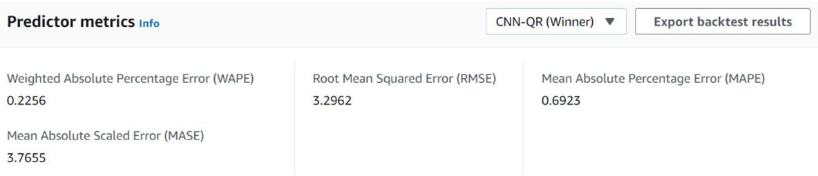
Figure 4.12 – The results page: Predictor metrics

Before we click on this button, first, let's define what backtesting is in the next section.

What is backtesting?

Backtesting is a technique used in time series-oriented machine learning to tune your model parameters during training and produce accuracy metrics. To perform backtesting, Amazon Forecast splits the data that you provide into two datasets:

• A training dataset, which is used to train a model
• A testing dataset, which is used to generate forecasts for data points within the testing set

Then, Amazon Forecasts computes the different accuracy metrics, as described earlier, by comparing how close the forecasted values are when compared with the actual values in the testing set. In the following diagram, you can see how a single backtest window is defined:

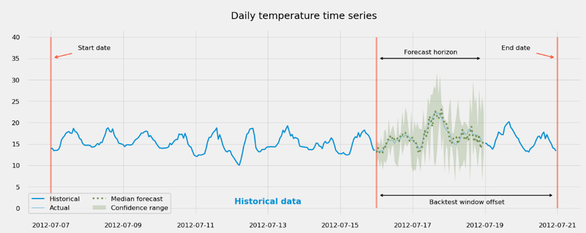
Figure 4.13 – Defining the backtest window length

In the preceding plot, you can see how Amazon Forecast would split your dataset to build a training dataset out of the historical data and a testing dataset out of data present in the forecast horizon. Note that in the preceding plot, the forecast horizon is shorter than the backtest window width: the latter is used to define the time split at which the forecast horizon starts. In this case, only part of the data present in the backtest window is used to build the testing dataset. If you want the testing dataset to leverage as much data as possible, you will have to set the backtest window to a width that is equal to the forecast horizon (which is the default value suggested by Amazon Forecast).

To train your first predictor, we leave the backtesting parameters at their default values. They are as follows:

• The number of backtest windows is 1.
• The length of the backtest window is equal to the forecast horizon. If you remember well, we selected a 30-day horizon, so our default backtest window length was also set to 30. You can adjust this value to request Amazon Forecast to use a larger backtest window than the forecast horizon. However, the backtest window length cannot be smaller than the requested forecast horizon.

In Chapter 5, Customizing Your Predictor Training, you will learn how you can adjust these parameters to improve your forecasting accuracy.

Exporting backtest results

Now, let's click on the Export backtest results button. You are brought to the following Export details screen:

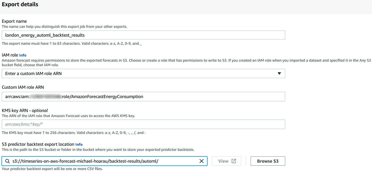
Figure 4.14 –Export details of backtest results

Important Note

In AutoML mode, backtest results are only available for the winning algorithm.

As you can see in the preceding screenshot, you need to fill in the following parameters:

• Export name: london_energy_automl_backtest_results
• IAM role: Select Enter a custom IAM role ARN and paste the ARN of the AmazonForecastEnergyConsumption role that you created in Chapter 3, Creating a Project and Ingesting Your Data, in the IAM service. As a reminder, the format of the ARN should be arn:aws:iam::<ACCOUNT-NUMBER>:role/AmazonForecastEnergyConsumption, where <ACCOUNT-NUMBER> needs to be replaced by your AWS account number.
• S3 predictor backtest export location: We are going to export our results in the same location where we put the datasets to be ingested. Fill in the following S3 URL: s3://<BUCKET>/backtest-results/automl/. Here, <BUCKET> should be replaced by the name of the bucket you created in Chapter 3, Creating a Project and Ingesting Your Data. Mine was called timeseries-on-aws-forecast-michael-hoarau, and the full URL where I want my backtest results to be exported will be s3:// timeseries-on-aws-forecast-michael-hoarau/backtest-results/automl/.

Click on the Start button to initiate the backtest results export. A blue ribbon at the top of the window informs you that a predictor backtest export is in progress. This process can take up to 15 to 20 minutes, after which we can go to the Amazon S3 console to collect our results.

In the upper-left corner of your AWS console, you will see a Services drop-down menu that will display all of the available AWS services. In the Storage section, look for the S3 service and click on its name to navigate to the S3 console. Click on the name of the bucket you used to upload your datasets to visualize its content:

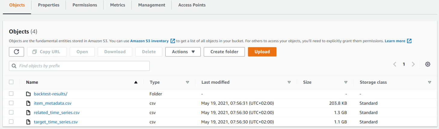
Figure 4.15 – Backtest results location on Amazon S3

On this screen, you will see a backtest-results/ folder. Click on it, and then click on the automl folder name. In this folder, you will find an accuracy-metrics-values folder and a forecasted-values folder.

We are going to take a look at the content of each of these folders next.

Backtest predictions overview

In the S3 listing of the backtest-results/ folder, click on the forecasted-values/ folder. You will end up inside a directory with a collection of CSV files:

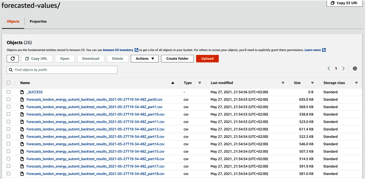
Figure 4.16 – Backtest forecast results as stored on Amazon S3

Each CSV file has a name that follows this pattern:

Forecasts_<export_name>_<yyyy-mm-ddTHH-MM-SSZ>_part<NN>

Here, export_name is the label you chose to name your backtest export job followed by a timestamp label (time at which the export was generated) and a part number label.

Each CSV file contains the backtest results for a subset of item_id (which, in our case, corresponds to the household ID). In the dataset we used, we had slightly more than 3,500 households and Amazon Forecast generated 25 files (from part0 to part24), each containing the backtest results for approximately 140 households.

Click on the checkbox next to the first CSV file and click on Download. This action will download the CSV file locally where you can open it with any spreadsheet software such as Excel or process it with your favorite programming language. I am going to open this file with Excel and plot the different time series available in these files for a few households. Click on the following link to download my Excel file and follow along with my analysis: https://packt-publishing-timeseries-on-aws-michaelhoarau.s3-eu-west-1.amazonaws.com/part1-amazon-forecast/london_energy_automl_backtest_results.xlsx

The raw data is located in the first tab (raw) and looks like this:

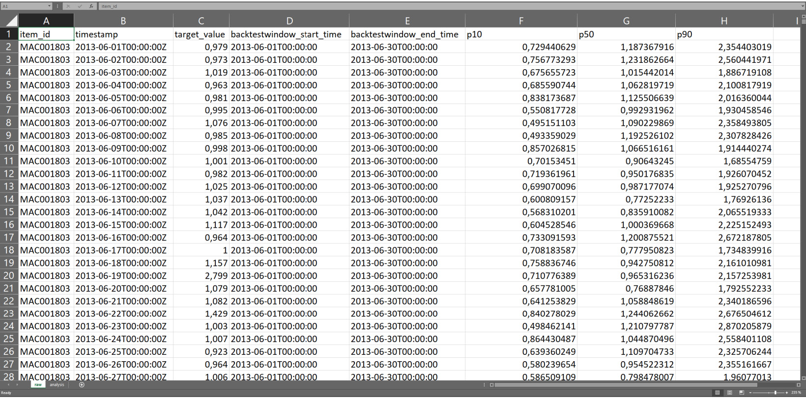
Figure 4.17 – Raw data from the backtest result

The different columns generated by Amazon Forecast are as follows:

• item_id: This column contains the ID of each household.
• timestamp: For each household, there will be as many data points as the length of the backtest window, as configured in the predictor training parameters. With a forecast frequency of 1 day and a backtest window length of 30, we end up with 30 data points. The timestamps from these columns will include 30 days worth for each household.
• target_value: This is the actual value as observed in the known historical time series data. This is the value that our predictions will be compared to in order to compute the error made by the model for a given data point.
• Backtestwindow_start_time and Backtestwindow_end_time: This is the start and end of the backtest window. At training time, you can request up to five backtest windows (we will see this in the advanced configuration in Chapter 5, Customizing Your Predictor Training). Backtest results will be available for all of the backtest windows.
• p10, p50, and p90: These are the values for each forecast type as requested at training time. You can request up to five forecast types, and they will all appear as individual columns in this file.

Now let's navigate to the second tab of the Excel file (called analysis): this tab leverages the raw data located in the first tab to plot the predictions obtained in the backtest window and offers a comparison with the actual data:

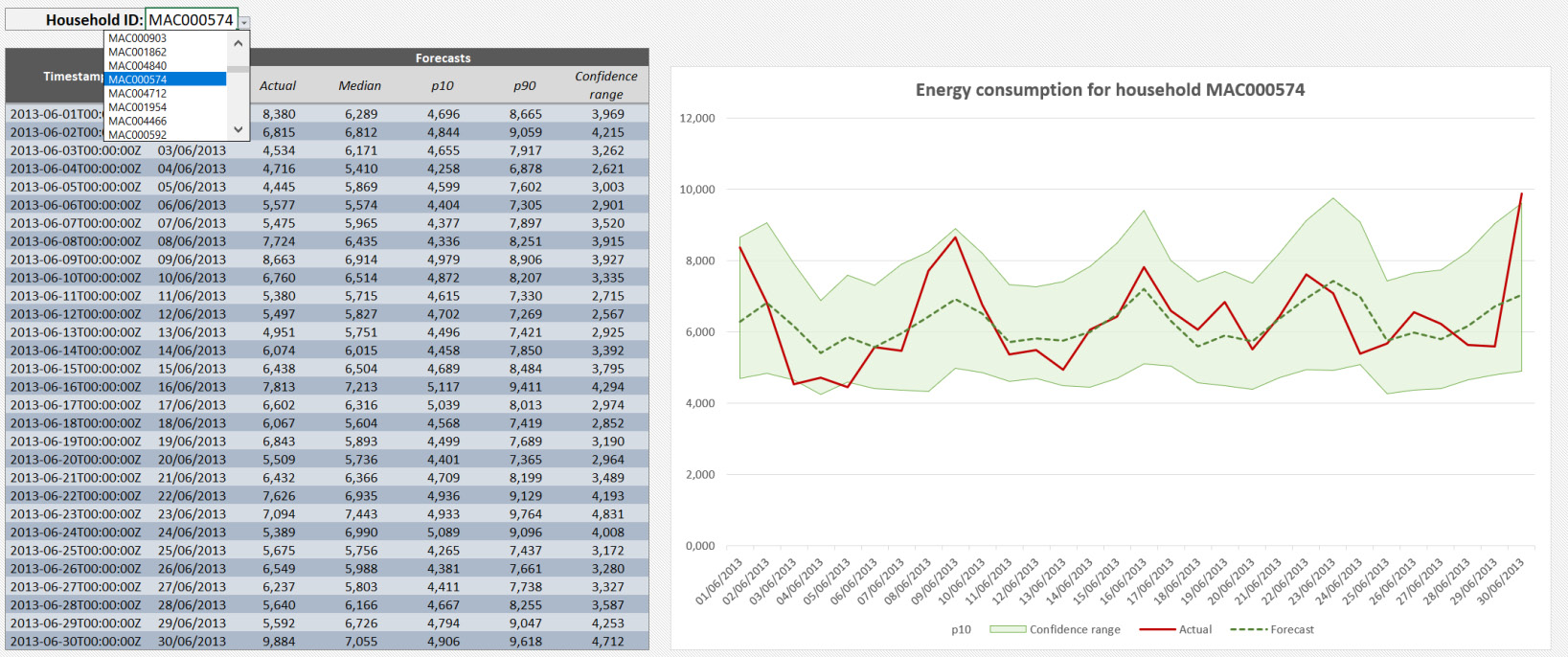
Figure 4.18 – The backtest analysis tab

Use the drop-down menu in the upper-left corner to select the household you want to analyze. The backtest result for this household is updated and the plot on the right reflects this change. Let's zoom into the backtest plot:

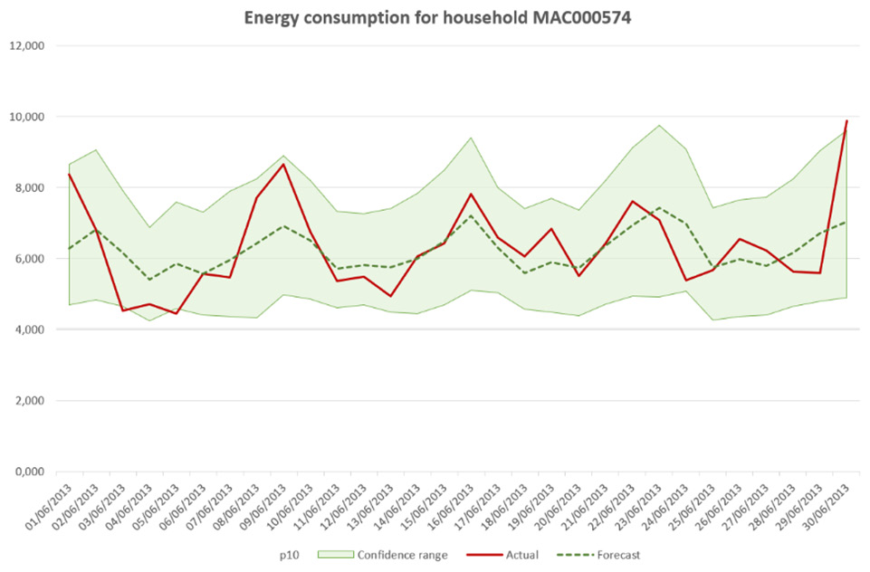
Figure 4.19 – The backtest analysis plot

On this plot, you can see three pieces of information:

• The actual energy consumption in the thick solid line.
• The predicted values in a dotted line: This is the median forecast (also called forecast type 0.5 or p50). This forecast type estimates a value that is lower than the observed value 50% of the time.
• The 80% confidence interval is represented as a shaded area around the median forecast. The lower bound of this confidence interval is the p10 forecast (the actual values are expected to be lower than this value 10% of the time), and the upper bound is the p90 forecast (for which the actual values are expected to be lower 90% of the time).

Feel free to explore further by selecting a different household to see what the backtest results look like.

Backtest accuracy overview

In the S3 listing of the backtest-results/ folder, click on the accuracy-metrics-values/ folder. You will end up inside a directory with a collection of CSV files with names that follow this pattern: Accuracy_<export_name>_<yyyy-mm-ddTHH-MM-SSZ>_part<NN>. Here, export_name is the label you chose to name your backtest export job followed by a timestamp label (the time at which the export was generated) and a part number label:

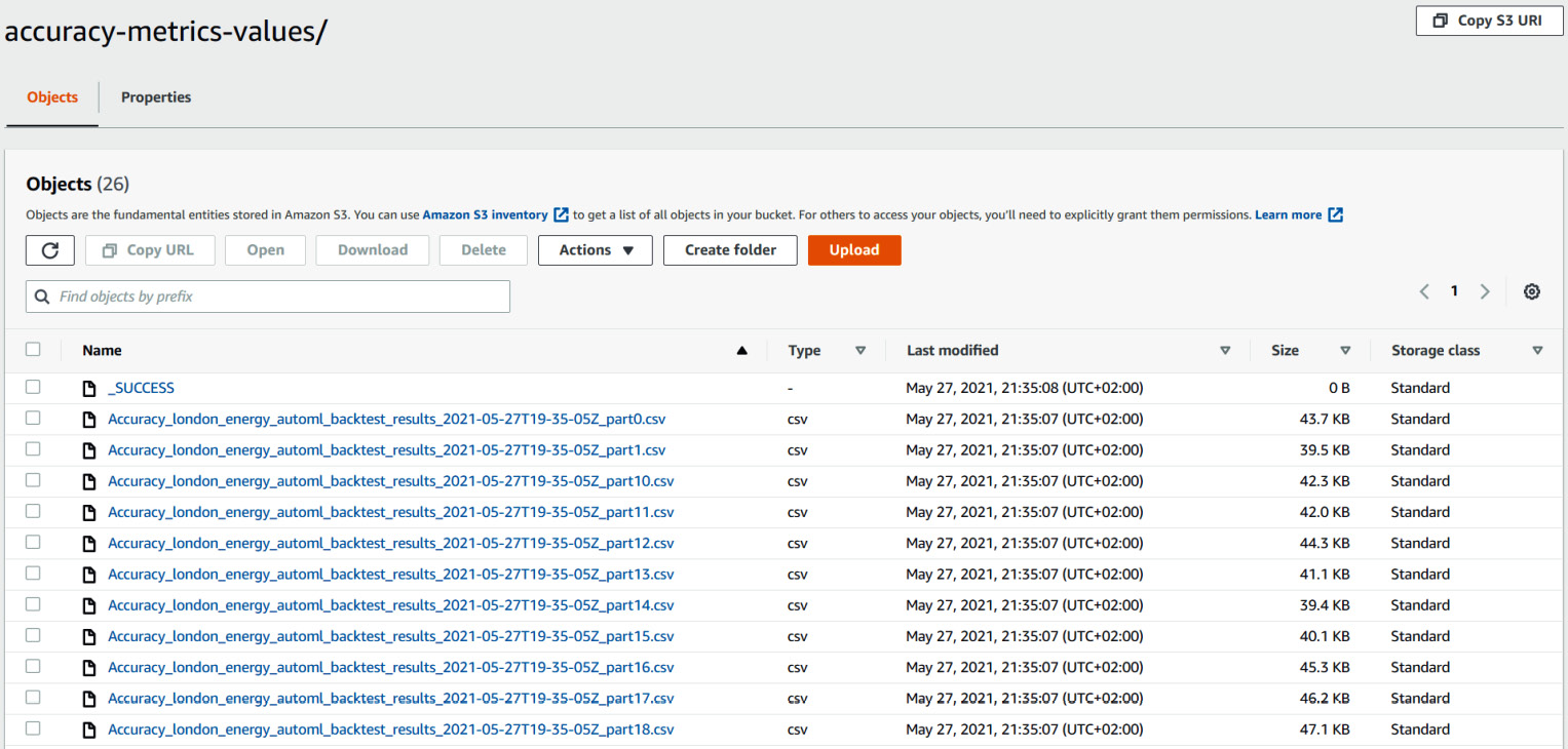
Figure 4.20 – The backtest accuracy results as stored on Amazon S3

Each CSV file contains the backtest accuracy results for a subset of item_id (which, in our case, corresponds to the household ID). In the dataset we used, we had slightly more than 3,500 households, and Amazon Forecast generated 25 files (from part0 to part24) with each containing the backtest results for approximately 140 households. If you want to have a complete overview of the accuracy metrics for all item_id types of your dataset, you will have to download and concatenate all the CSV files (or perform this action programmatically).

Click on the checkbox next to the first CSV file and click on Download. This action will download the CSV file locally where you can open it with any spreadsheet software such as Excel or process it with your favorite programming language.

For the analysis we just performed, I concatenated all of the accuracy metrics files and made them available in the following link. Feel free to download and open this file to follow along with my analysis: https://packt-publishing-timeseries-on-aws-michaelhoarau.s3-eu-west-1.amazonaws.com/part1-amazon-forecast/london_energy_automl_backtest_accuracy_metrics.csv

The raw data provided by Amazon Forecast is located in the first tab and contains the accuracy metric computed for each item_id time series, as shown in the following screenshot:

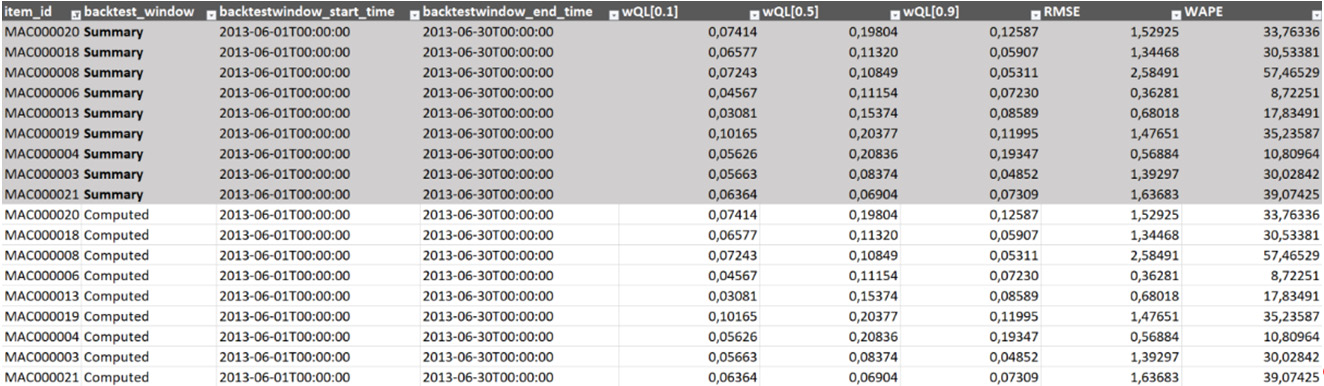
Figure 4.21 – The backtest accuracy metrics raw data

Note

If you open the CSV file with spreadsheet software such as Microsoft Excel, you will have to transform the text into columns and select comma as the separator (you will find this feature in the Data tab of Microsoft Excel). Depending on the regional parameters of your local stations, you might also have to explicitly specify the decimal separator you want to use for all the wQL columns. This is so that Excel treats them as numerical values and not strings of text.

For each item_id time series, you will find the metrics computed for the following:

• Each backtest window (we can have up to five, which will yield five rows for each item_id time series in this file)
• The summary (this is the average over all of the requested backtest windows, the grayed-out area in the previous diagram)

The metrics computed for each household are the ones shown in the console: the weighted quantile for each forecast type (if you kept the default parameters, this will be wQL[0.1], wQL[0.5], and wQL[0.9]), the RMSE, and the WAPE.

Summary

Congratulations! In this chapter, you trained your first predictor with Amazon Forecast. You learned how to configure a predictor with the default training parameters and developed a sound command regarding how a trained predictor can be evaluated through different metrics such as the wQL, the WAPE, or the RMSE. Additionally, you learned how to download the evaluations of a trained model to finely analyze your predictor results with your favorite spreadsheet tool.

In the next chapter, you will learn how to leverage all the flexibility Amazon Forecast can provide you to customize and further enhance your predictors to better suit your data.