Chapter 5: Customizing Your Predictor Training

In the previous chapter, you trained your first predictor on a household energy consumption dataset. You used the fully automated machine learning (AutoML) approach offered by default by Amazon Forecast, which let you obtain an accurate forecast without any ML or statistical knowledge about time series forecasting.

In this chapter, you will continue to work on the same datasets, but you will explore the flexibility that Amazon Forecast gives you when training a predictor. This will allow you to better understand when and how you can adjust your forecasting approach based on specificities in your dataset or specific domain knowledge you wish to leverage.

In this chapter, we're going to cover the following main topics:

• Choosing an algorithm and configuring the training parameters
• Leveraging hyperparameter optimization (HPO)
• Reinforcing your backtesting strategy
• Including holiday and weather data
• Implementing featurization techniques
• Customizing quantiles to suit your business needs

Technical requirements

No hands-on experience of a language such as Python or R is necessary to follow along with the content from this chapter. However, we highly recommend that you read this chapter while being connected to your own Amazon Web Services (AWS) account and open the Amazon Forecast console to run the different actions on your end.

To create an AWS account and log in to the Amazon Forecast console, you can refer to the Technical requirements section of Chapter 2, An Overview of Amazon Forecast.

The content in this chapter assumes that you have a dataset already ingested and ready to be used to train a new predictor. If you don't, I recommend that you follow the detailed process detailed in Chapter 3, Creating a Project and Ingesting your Data. You will need the Simple Storage Service (S3) location of your three datasets, which should look like this (replace <YOUR_BUCKET> with the name of the bucket of your choice):

• Target time series: s3://<YOUR_BUCKET>/target_time_series.csv
• Related time series: s3://<YOUR_BUCKET>/related_time_series.csv
• Item metadata: s3://<YOUR_BUCKET>/item_metadata.csv

You will also need the Identity and Access Management (IAM) role you created to let Amazon Forecast access your data from Amazon S3. The unique Amazon Resource Number (ARN) of this role should have the following format: arn:aws:iam::<ACCOUNT-NUMBER>:role/AmazonForecastEnergyConsumption. Here, you need to replace <ACCOUNT-NUMBER> with your AWS account number.

With this information, you are now ready to dive into the more advanced features offered by Amazon Forecast.

Choosing an algorithm and configuring the training parameters

In Chapter 4, Training a Predictor with AutoML, we let Amazon Forecast make all the choices for us and left all the parameters at their default values, including the choice of algorithm. When you follow this path, Amazon Forecast applies every algorithm it knows on your dataset and selects the winning one by looking at which one achieves the best average weighted absolute percentage error (WAPE) metric in your backtest window (if you kept the default choice for the optimization metric to be used).

At the time of writing this chapter, Amazon Forecast knows about six algorithms. The AutoML process is great when you don't have a precise idea about the algorithm that will give the best result with your dataset. The AutoPredictor settings also give you the flexibility to experiment easily with an ensembling technique that will let Amazon Forecast devise the best combination of algorithms for each time series of your dataset. However, both these processes can be quite lengthy as they will, in effect, train and evaluate up to six models to select only one algorithm at the end (for AutoML) or a combination of these algorithms for each time series (for AutoPredictor).

Once you have some experience with Amazon Forecast, you may want to cut down on this training time (which will save you both time and training costs) and directly select the right algorithm among the ones available in the service.

When you open the Amazon Forecast console to create a new predictor and disable the AutoPredictor setting, you are presented with the following options in an Algorithm selection dropdown:

Figure 5.1 – Manual algorithm selection

In this chapter, we will dive into each of the following algorithms:

• Exponential smoothing (ETS)
• Autoregressive integrated moving average (ARIMA)
• Non-parametric time series (NPTS)
• Prophet
• DeepAR+
• Convolutional Neural Network-Quantile Regression (CNN-QR)

For each of these, I will give you some theoretical background that will help you understand the behaviors these algorithms are best suited to capture. I will also give you some pointers about when your use case will be a good fit for any given algorithm.

ETS

ETS stands for Error, Trend, and Seasonality: ETS is part of the exponential smoothing family of statistical algorithms. These algorithms work well when the number of time series is small (fewer than 100).

The idea behind exponential smoothing is to use a weighted average of all the previous values in a given time series, to forecast future values. This approach approximates a given time series by capturing the most important patterns and leaving out the finer-scale structures or rapid changes that may be less relevant for forecasting future values.

The ETS implementation of Amazon Forecast performs exponential smoothing accounting for trends and seasonality in your time series data by leveraging several layers of smoothing.

Theoretical background

Trend and seasonal components can be additive or multiplicative by nature: if we consume 50% more electricity during winter, the seasonality is multiplicative. On the other hand, if we sell 1,000 more books during Black Friday, the seasonality will be additive.

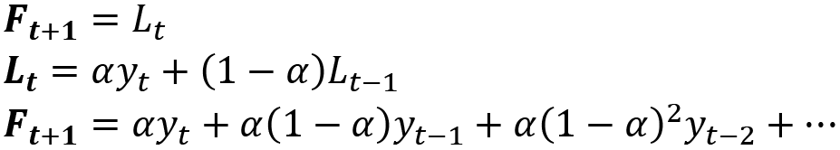
Let's call yt the raw values of our initial time series and let's decompose the different smoothing layers in the case of additive trend and seasonality, as follows:

1. We first start by applying a moving average (MA) on our time series. If W is the width of the rolling window and yt the different timesteps of our time series, then the MA computed at time t will give us the predicted forecast Ft+1 at time t+1 and is given by the following formula:

2. The MA step gives the same importance (weight) to each of the previous timesteps that fall in the rolling window width. Adding a smoothing constant will give more weight to recent values while reducing the impact of the window width choice. Let's call our smoothing constant : this value, set between 0 and 1, will be a parameter telling our model how fast we want to forget the previous values of the time series. This can also be called a baseline factor as it's used to model the base behavior our forecast will have. In the following formula, you will notice that the previous timesteps are now weighted with a weight that is exponentially decreasing. Our forecast baseline at time t+1 can be derived from the series level at the previous timestep, Lt:

When a trend component is present in our time series, the previous approach does not do well: to counter this, we add a trend smoothing parameter, generally called , that we apply in a similar fashion on the difference between successive timesteps on our series. is also set between 0 and 1. This yields to the double exponential smoothing, and the point forecast k periods ahead can be derived from both the series level and the series slope at the previous timestep Lt and Bt, as illustrated in the following formula:

If our signal also contains additional high-frequency (HF) signals such as a seasonality component, we need to add a third exponential smoothing parameter, usually called , and call the seasonal smoothing parameter (also set between 0 and 1 as and ). If m denotes the number of seasons to capture our new point forecast k periods ahead, this can now be derived with the triple exponential smoothing, using the series level Lt, the series slope Bt, and the seasonal component St at the previous timestep, as follows:

The ETS algorithm is also able to apply a damping parameter when there is a trend in a time series. When computing several periods ahead (in other words, when predicting a forecast horizon of several timesteps), we use the same slope as determined at the end of the historical time series for each forecast period. For long forecast periods, this may seem unrealistic, and we might want to dampen the detected trend as the forecast horizon increases. Accounting for this damping parameter (strictly set between and 1), the previous equations become these:

Implementation in Amazon Forecast

When Amazon Forecast trains a model with ETS, it uses the default parameters of the ets function available in the R forecast package. This means that all the ets parameters are automatically estimated. In addition, Amazon Forecast also automatically selects the model type according to the following criteria:

• With or without trend or seasonality
• Additive or multiplicative trend and seasonality
• Applying damping or not

All of these choices are abstracted away from you: multiple models are run behind the scenes and the best one is selected.

Amazon Forecast will create a local model for each time series available in your dataset. In the energy consumption example we have been running, each household electricity consumption would be modeled as a single ETS model.

If you want to get more in-depth details about the different exponential smoothing methods (including details of the equations when considering damping, and multiplicative trends and seasonality), how all these parameters are automatically computed, and which variation is automatically selected, I recommend you deep dive into this paper by Rob Hyndman et. al: A state space framework for automatic forecasting using exponential smoothing methods. Here is a persistent link to this paper: https://doi.org/10.1016/S0169-2070(01)00110-8.

ARIMA

With ETS, ARIMA is another very well-known family of flexible statistical forecasting models. ARIMA is a generalization of the ARMA family of models, where ARMA describes a time series with two polynomials: one for autoregression and the other for the MA.

Although all these family of models involves inputting many parameters and computing coefficients, Amazon Forecast leverages the auto.arima method from the forecast R package available on the Comprehensive R Archive Network (CRAN). This method conducts a search over the possible values of the different ARIMA parameters to identify the best model of this family.

Theoretical background

Let's call yt the raw values of our initial time series and let's decompose the different steps needed to estimate an ARIMA model, as follows:

1. We start by making the time series stationary by using differencing. In statistics, this transformation is applied to non-stationary time series to remove non-constant trends. In the ARIMA implementation of Amazon Forecast, differencing is applied once (first-order differencing ) or twice (second-order differencing ) and is the reason why the model is called integrated (the I in ARIMA stands for integrated). The formula is provided here:

2. We then use this differenced data to build an autoregressive (AR) model that specifies that our prediction depends linearly on the previous timesteps and on a random term. Let's call Yt (with a capital Y) the differenced data obtained after the integrated step of the algorithm (Yt will either be or , depending on the differencing order retained in the previous step). An AR model of order p can be written as a function of previous terms of the series and of a series of coefficients to , as shown in the following formula:

3. Once we have an AR model, we use an MA model to capture the dependency of our prediction on the current and previous values of the random term. An MA model of order q can be written as a function of the mean µ of the series and of a list of parameters to applied to random error terms to , as shown in the following formula:

4. When putting together an AR model and an MA model after differencing, we end up with the following estimation for the ARIMA model:

Implementation in Amazon Forecast

When Amazon Forecast trains a model with ETS, it uses the default parameters of the arima function available in the R forecast package. Amazon Forecast also uses the auto.arima method, which conducts a search of the parameter space to automatically find the best ARIMA parameters for your dataset. This includes exploring a range of values for the following:

• The differencing degree
• The AR order
• The MA order

This means that all these arima parameters are automatically estimated and that the model type is also automatically selected: all of these choices are abstracted away from you as multiple models are run behind the scenes, and the best one is selected.

Amazon Forecast will create a local model for each time series available in your dataset. In the energy consumption example we have been running, each household electricity consumption would be modeled as a single ARIMA model.

If you want to get more in-depth details about the automatic parameter choice from ARIMA, I recommend that you deep dive into this paper by Hyndman and Khandakar: Automatic Time Series Forecasting: The forecast Package for R. Here is a persistent link to this paper: https://doi.org/10.18637/jss.v027.i03.

NPTS

A simple forecaster is an algorithm that uses one of the past observed values as the forecast for the next timestep, as outlined here:

• A naïve forecaster takes the immediately previous observation as the forecast for the next timestep.
• A seasonal naïve forecaster takes the observation of the past seasons as the forecast for the next timestep.

NPTS falls into this class of simple forecaster.

Theoretical background

As just mentioned, NPTS falls in the simple forecasters' category. However, it does not use a fixed time index as the last value: rather, it samples randomly one of the past values to generate a prediction. By sampling multiple times, NPTS is able to generate a predictive distribution that Amazon Forecast can use to compute prediction intervals.

Let's call the raw values of our initial time series, with t ranging from 0 to T – 1 and T being the time step for which we want to deliver a prediction , as follows:

And the time index t is actually sampled from a sampling distribution qT. NPTS uses the following sampling distribution:

Here, is a kernel weight hyperparameter that should be adjusted based on the data and helps you control the amount of decay in the weights. This allows NPTS to sample recent past values with a higher probability than observations from a distant past.

This hyperparameter can take values from 0 to infinitum. Here are the meanings of these extreme values:

• When if 0, then all the weights are uniform: this leads to the climatological forecaster. The predicted value is sampled uniformly from the past, only accounting for the statistical distribution of values a given time series can time, without considering the dynamical implications of the current behavior.
• If is set to infinitum, you get the naïve forecaster, which always predicts the last observed value.

Once you have generated a prediction for the next step, you can include this prediction in your past datasets and generate subsequent predictions while giving the ability to NPTS to sample past predicted data.

If you want to get in-depth details about this algorithm and, more generally, about intermittent data forecasting, you can dive deeper into the following articles:

• GluonTS: Probabilistic Time Series Models in Python (https://arxiv.org/pdf/1906.05264.pdf)
• Intermittent Demand Forecasting with Renewal Processes (https://arxiv.org/pdf/2010.01550.pdf)

Let's now have a look at how this algorithm has been implemented in Amazon Forecast.

Implementation in Amazon Forecast

Here are the key parameters the NPTS algorithm lets you select:

• context_length: This is the number of data points in the past NPTS uses to make a prediction. By default, Amazon Forecast uses all the points in the training range.
• kernel_type: This is the method used to define weights to sample past observations. This parameter can either be uniform or exponential. The default value is exponential.
• exp_kernel_weights: When you choose an exponential kernel type, you can specify the parameter to control how fast the exponential decay is applied to past values. The default value for this parameter is 0.01. This parameter should always be a positive number.
• You can also choose to sample only the past seasons instead of sampling from all the available observations. This behavior is controlled by the use_seasonal_model parameter, which can be set to True (which is the default value) or False.

When a seasonal model is used, you also have the ability to request Amazon Forecast to automatically provide and use seasonal features that depend on the forecast granularity by setting the use_default_time_features parameter to True. Let's say, for instance, that your data is available at the hourly level: if this parameter is set to True and you want to give a prediction for 3 p.m., then the NPTS algorithm will only sample past observations that also happened at 3 p.m.

Prophet

Prophet is a forecasting algorithm that was open sourced by Facebook in February 2017.

Theoretical background

The Prophet algorithm is similar to generalized additive models with four components, as follows:

Here, the following applies:

• g(t) is the trend function: trends are modeled with a piecewise logistic growth model. Prophet also allows trends to change through automatic changepoint selection (by defining a large number of changepoints—for instance, one per month). The logistic growth model is defined using the capacity C(t) (what the maximum market size is in terms of the number of events measured), the growth rate k, and an offset parameter m, as follows:

• s(t) represents periodic changes such as yearly or weekly seasonal components. If P is the regular period you expect your time series to have (P = 365.25 for yearly seasonal effect and P =7 for weekly periods), an approximate arbitrary smooth seasonal effect can be defined, such as this:

By default, Prophet uses N = 10 for yearly seasonality and N = 3 for weekly seasonality.

• h(t) represents the effect of holidays or, more generally, irregular events over 1 or more days. Amazon Forecast feeds this field with a list of holidays when you decide to use the Holidays supplementary feature (see the Including holidays and weather data section later in this chapter).
• is an error term accounting for everything that is not accommodated by the model.

If you want to know more about the theoretical details of Prophet, you can read through the original paper published by Facebook available at the following link: https://peerj.com/preprints/3190/.

Implementation in Amazon Forecast

Amazon Forecast uses the Prophet class of the Python implementation of Prophet using all the default parameters.

Amazon Forecast will create a local model for each time series available in your dataset. In the energy consumption example we have been running, each household electricity consumption would be modeled as a single Prophet model.

If you want to get more in-depth details about the impact of the default parameter choice from Prophet, I recommend that you read through the comprehensive Prophet documentation available at the following link: https://facebook.github.io/prophet/.

DeepAR+

Classical methods we have been reviewing—such as ARIMA, ETS, or NPTS—fit a single model to every single time series provided in a dataset. They then use each of these models to provide a prediction for the desired time series. In some applications, you may have hundreds or thousands of similar time series that evolve in parallel. This will be the case of the number of units sold for each product on an e-commerce website or the electricity consumption of every household served by an energy provider. For these cases, leveraging global models that learn from multiple time series jointly may provide more accurate forecasting. This is the approach taken by DeepAR+.

Theoretical background

DeepAR+ is a supervised algorithm for univariate time series forecasting. It uses recurrent neural networks (RNNs) and a large number of time series to train a single global model. At training time, for each time series ingested into the target time series dataset, DeepAR+ generates multiple sequences (time series snippets) with different starting points in the original time series to improve the learning capacity of the model.

The underlying theoretical details are beyond the scope of this book: if you want to know more about the theoretical details of the DeepAR algorithm, you can do the following:

• You can head over to this YouTube video to understand how artificial networks can be adapted to sequences of data (such as time series): https://www.youtube.com/watch?v=WCUNPb-5EYI. This video is part of a larger course about ML and artificial neural networks (ANNs).
• You can read through the original published paper, DeepAR: Probabilistic Forecasting with Autoregressive Recurrent Networks by David Salinas, Valentin Flunkert, Jan Gasthaus, available at the following link: https://arxiv.org/abs/1704.04110.
• The DeepAR+ section of the Amazon Forecast documentation is very detailed, with many illustrations. You can directly follow this link: https://docs.aws.amazon.com/forecast/latest/dg/aws-forecast-recipe-deeparplus.html.

Implementation in Amazon Forecast

The key parameters the DeepAR+ algorithm lets you select are listed here:

• context_length: This is the number of data points in the past DeepAR+ uses to make a prediction. Typically, this value should be equal to the forecast horizon. DeepAR+ automatically feeds lagged values from the target time series data, so your context length can be much smaller than the seasonality present in your dataset.
• number_of_epochs: In ML, the learning process goes over the training data a certain number of times. Each pass is called an epoch. number_of_epochs has a direct impact on the training time, and the optimal number will depend on the size of the dataset and on the learning_rate parameter.
• likelihood: Amazon Forecast generates probabilistic forecasts and provides quantiles of the distribution. To achieve this, DeepAR+ uses different likelihoods (these can be seen as "noise" models) to estimate uncertainty, depending on the behavior of your data. The default value is student-T (which is suitable for real-valued data or sparse spiky data). Other possible values are beta (real values between 0 and 1), deterministic-L1 (to generate point forecasts instead of probabilistic ones), gaussian (for real-valued data), negative-binomial (for non-negative data such as count data), or piecewise-linear (for flexible distributions).

DeepAR+ also lets you customize the learning parameters, as follows:

• learning_rate: In ML-based algorithms, the learning rate is used to define the step size used at each iteration to try to reach an optimum value for a loss function. The greater the learning rate, the faster newly learned information overrides past learnings. Setting a value for the learning rate is a matter of compromise between moving too fast at the risk of missing optimal values of the model parameters or moving too slowly, making the learning too long. The default value for DeepAR+ is 0.001.
• max_learning_rate_decays: ML model learning can be nonlinear. At the beginning of the process, you can explore faster and have a high learning rate, whereas you may need to reduce the learning speed when you're approaching an optimal value of interest. This parameter defines the number of times the learning rate will be decayed during training. This is disabled by default (0). If this parameter is set to 3 (for instance), and you train your model over 100 epochs, then the learning rate will be decayed once after 25, 50, and 75 epochs (3 decaying episodes).
• learning_rate_decay: This parameter defines the factor used to multiply the current learning rate when a decay is triggered. This decay will be applied a number of times, defined by the max_learning_rate_decays parameter. The default value is 0.5. In the previous example, where 3 decaying episodes occurred over the course of 100 epochs, if the learning_rate parameter starts at 0.1, then it will be reduced to 0.05 after 25 epochs, to 0.025 after 50 epochs, and to 0.0125 after 75 epochs.

The architecture of the model can be customized with the following two parameters:

• The hidden layers of the RNN model from DeepAR+ can be configured by the number of layers (num_layers), and each layer can contain a certain number of long short-term memory (LSTM) cells (num_cells).
• num_averaged_models: During a given training process, DeepAR+ can encounter several models that have a close overall performance but different accuracy at the individual time series level. DeepAR+ can average (ensemble) different model behaviors to take advantage of the strength of up to five models.

CNN-QR

CNN-QR leverages a similar approach to DeepAR+, as it also builds a global model, learning from multiple time series jointly to provide more accurate forecastings.

Theoretical background

CNN-QR is a sequence-to-sequence (Seq2Seq) model that uses a large number of time series to train a single global model. In a nutshell, this type of model tests how well a prediction reconstructs a decoding sequence conditioned on an encoding sequence. It uses a quantile decoder to make multi-horizon probabilistic predictions.

The underlying theoretical details are beyond the scope of this book, but if you want to know more about some theoretical work leveraged by algorithms such as CNN-QR, you can read through the following sources:

• A Multi-Horizon Quantile Recurrent Forecaster (https://arxiv.org/pdf/1711.11053.pdf).
• The Amazon Forecast documentation, which is very detailed with many illustrations. You can directly follow this link: https://docs.aws.amazon.com/forecast/latest/dg/aws-forecast-algo-cnnqr.html.

Implementation in Amazon Forecast

The key parameters the DeepAR+ algorithm lets you select are these:

• context_length: This is the number of data points in the past CNN-QR uses to make a prediction. Typically, this value should be within 2 and 12 times the forecast horizon. Contrary to DeepAR+, CNN-QR does not automatically feed lagged values from the target time series data, so this parameter will usually be larger than with DeepAR+. Context length can be much smaller than the seasonality present in your dataset.
• number_of_epochs: In ML, the learning process goes over the training data a certain number of times. Each pass is called an epoch. number_of_epochs has a direct impact on the training time, and the optimal number will depend on the size of the dataset.
• use_related_data: This parameter will tell Amazon Forecast to use all the related time series data (ALL), none of them (NONE), only related data that does not have values in the forecast horizon (HISTORICAL), or only related data present both in the past and in the forecast horizon (FORWARD_LOOKING).
• use_item_metadata: This parameter will tell Amazon Forecast to use all provided item metadata (ALL) or none of it (NONE).

When should you select an algorithm?

The Amazon Forecast documentation includes a table to help you compare the different built-in algorithms used by this service. I recommend you refer yourself to it, as new approaches and algorithms may have been included in the service since the time of writing this book. You can find it at this link: https://docs.aws.amazon.com/forecast/latest/dg/aws-forecast-choosing-recipes.html.

Based on the algorithms available at the time of writing, I expanded this table to add a few other relevant criteria. The following table summarizes the best algorithm options you can leverage, depending on the characteristics of your time series datasets:

Figure 5.2 – Algorithm selection cheat sheet

Let's now expand beyond this summary table and dive into some specifics of each of these algorithms, as follows:

• ARIMA, ETS, and NPTS: These algorithms are quite low-computationally-intensive and can give you a robust baseline for your forecasting problem.
• ARIMA: The ARIMA algorithm parameters are not tunable by the HPO process, as the auto.arima method from the Forecast R package takes care of it to identify the most suitable parameters.
• NPTS: Amazon Forecast AutoML sometimes chooses NPTS when you know it is not the best fit. What happens is that your data may appear sparse at a certain granularity: if you train a predictor with AutoML, it may select NPTS, even though you have hundreds of individual time series that a deep neural network (DNN) could learn better from. One approach to let AutoML select an algorithm with a larger learning capacity is to aggregate your data at high granularity (for instance, summing hourly data to build a daily dataset).
• Prophet: This algorithm is a great fit for datasets that exhibit multiple strong seasonal behaviors at different scales and contain an extended time period (preferably at least a year for hourly, daily, or weekly data). Prophet is also very good at capturing the impact of important holidays that occur at irregular intervals and that are known in advance (yearly sporting events at varying dates). If your datasets include large periods of missing values or large outliers, have non-linear growth trends, or saturate values while approaching a limit, then Prophet can also be an excellent candidate.

Now that you know how to select an algorithm suitable for your business needs, let's have a look at how you can customize each of them and override the default parameters we left as is when you trained your first predictor in the previous chapter.

Leveraging HPO

Training an ML model is a process that consists of finding parameters that will help the model to better deal with real data. When you train your own model without using a managed service such as Amazon Forecast, you can encounter three types of parameters, as follows:

• Model selection parameters: These are parameters that you have to fix to select a model that best matches your dataset. In this category, you will find the , , , and parameters from the ETS algorithm, for instance. Amazon Forecast implements these algorithms to ensure that automatic exploration is the default behavior for ETS and ARIMA so that you don't have to deal with finding the best values for these by yourself. For other algorithms (such as NPTS), good default parameters are provided, but you have the flexibility to adjust them based on the inner knowledge of your datasets.
• Coefficients: These are values that are fitted to your data during the very training of your model. These coefficients can be the weights and biases of a neural network or the to coefficients of the MA part of ARIMA. Once these values have been fitted to your training data, their values define your model, and this set of values constitutes the main artifact that Amazon Forecast saves in the Predictor construct.
• Hyperparameters: These parameters control the learning process itself. The number of iterations (epochs) to train a deep learning (DL) model or the learning rate are examples of hyperparameters you can tweak to adjust your training process.

Amazon Forecast endorses the responsibility to manage the model selection parameters and coefficients for you. In the AutoML process, it also uses good default values for the hyperparameters of each algorithm and applies HPO for the DL algorithms (DeepAR+ and CNN-QR) to make things easier for you.

When you manually select an algorithm that can be tuned, you can also enable an HPO process to fine-tune your model and reach the same performance as with AutoML, but without the need to train a model with each of the available algorithms.

What is HPO?

In learning algorithms such as the ones leveraged by Amazon Forecast, HPO is the process used to choose the optimal values of the parameters that control the learning process.

Several approaches can be used, such as grid search (which is simply a parameter sweep) or random search (selecting hyperparameter combinations randomly). Amazon Forecast uses Bayesian optimization.

The theoretical background of such an optimization algorithm is beyond the scope of this book, but simply speaking, HPO matches a given combination of parameter values with the learning metrics (such as WAPE, weighted quantile loss (wQL), or root mean square error (RMSE), as mentioned in Chapter 4, Training a Predictor with AutoML). This matching is seen as a function by Bayesian optimization, which tries to build a probabilistic model for it. The Bayesian process iteratively updates hyperparameter configuration and gathers information about the location of the optimum values of the matching functions modeled.

To learn more about HPO algorithms, you can read through the following article: https://proceedings.neurips.cc/paper/2011/file/86e8f7ab32cfd12577bc2619bc635690-Paper.pdf.

If you want to read more about Bayesian optimization and why it is better than grid search or random search, the following article will get you started:

Practical Bayesian Optimization of ML Algorithms (https://arxiv.org/abs/1206.2944)

Let's now train a new predictor, but explicitly using HPO.

Training a CNN-QR predictor with HPO

In this section, we are going to train a second predictor, using the winning algorithm found in Chapter 4, Training a Predictor with AutoML. As a reminder, the winning algorithm was CNN-QR and we achieved the following performance:

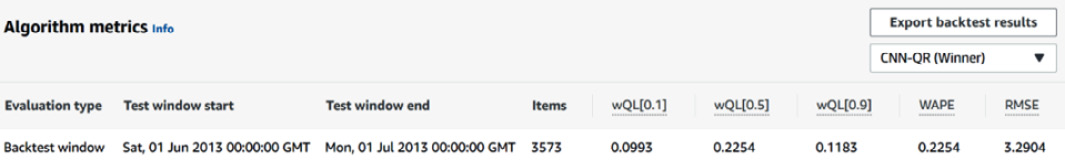
Figure 5.3 – Winning algorithm performance with AutoML

To train a new predictor, log in to the AWS console, navigate to the Amazon Forecast console, and click on the View dataset groups button. There, you can click on the name of the dataset group you created in Chapter 3, Creating a Project and Ingesting your Data. Check out this chapter if you need a reminder on how to navigate through the Amazon Forecast console. You should now be on the dashboard of your dataset group, where you will click on the Train predictor button, as illustrated in the following screenshot:

Figure 5.4 – Dataset group initial dashboard

Once you click the Train predictor button, the following screen will open up to let you customize your predictor settings:

Figure 5.5 – Predictor settings

For your Predictor settings options, we are going to fill in the following parameters:

• Predictor name: london_energy_cnnqr_hpo.
• Forecast frequency: We will keep the same frequency as before, which is also the original frequency of the ingested data. Let's set this parameter to 1 day.
• Forecast horizon: 30. As the selected forecast horizon is 1 day, this means that we want to train a model that will be able to generate the equivalent of 30 days' worth of data points in the future. We want to compare the performance of our initial predictor with this new one, so let's keep the same horizon to make this comparison more relevant.
• Forecast quantiles: Leave the settings at their default values, with three quantiles defined at 0.10, 0.50, and 0.90. We will detail this setting later in this chapter.

In the next section, disable the AutoPredictor toggle and select CNN-QR in the Algorithm selection dropdown.

Click on Perform hyperparameter optimization (HPO). A new section called HPO Config appears, where you can decide the range of values you want Amazon Forecast to explore for the different tunable hyperparameters of CNN-QR. This configuration must be written in JavaScript Object Notation (JSON) format.

Let's enter the following JSON document into the HPO Config widget:

{

  "ParameterRanges": {

    "IntegerParameterRanges": [

      {

        "MaxValue": 360,

        "MinValue": 60,

        "ScalingType": "Auto",

        "Name": "context_length"

      }

    ]

  }

}

With this configuration, we are telling Amazon Forecast that we want it to explore a hyperparameter space defined by these potential values:

• context_length will evolve between MinValue=60 days and MaxValue=360 days.
• The HPO process will also automatically try four different configurations of related datasets: no related dataset used (NONE), all of them (ALL), use the related dataset that only contains historical values (HISTORICAL), or use the related datasets that contain both past historical values and future values (FORWARD_LOOKING).
• It will also automatically try two different configurations of item metadata: no metadata used (NONE) or all metadata used (ALL).

In the Training parameters section, we will leave the epochs number at 100 (a similar number to the default value used by the AutoML procedure) for comparison purposes, as follows:

{

  "epochs": "100"

  [...]

}

Leave all the other parameters at their default values and click Create to start the training of our new predictor with the HPO procedure. Our predictor will be created with the Create in progress status, as illustrated in the following screenshot:

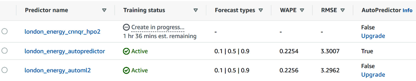
Figure 5.6 – CNN-QR predictor training with HPO in progress

After a while (a little less than 2 hours, in my case), our new predictor is trained and ready to be used, as can be seen here:

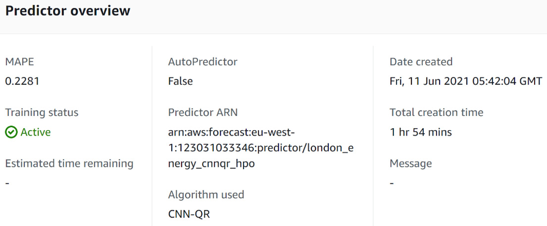
Figure 5.7 – Trained CNN-QR predictor

In your case, the mean-absolute percentage error (MAPE) metric may be slightly different but will be close to the number you see here. You can see that in my case, I obtained a MAPE value of 0.2281, which is extremely close to the value obtained in the AutoML process (which was 0.2254). As explained in the What is HPO? section, the slight differences come from the random nature of the Bayesian procedure.

You now know how to configure HPO to your predictor training. However, not all algorithms can be fine-tuned using this process, and not all parameters can be defined as targets with ranges to explore. In the next section, we will look at the options you have for each algorithm.

Introducing tunable hyperparameters with HPO

When you know which algorithm will give the best results for your datasets, you may want to ensure that you get the most out of this algorithm by using HPO. Let's have a look at what is feasible for each algorithm, as follows:

• ETS: HPO is not available in Amazon Forecast. However, the service leverages the default parameters from the ets module from the forecast R package: the latter takes an argument called model that is set to ZZZ by default. When this is the case, the model argument is automatically selected to provide the best-performing ETS model.
• NPTS: HPO is not available for NPTS. To train different types of NPTS models, you can train separate predictors with different training parameters on the same dataset group.
• ARIMA: HPO is not available in Amazon Forecast. However, Amazon Forecast leverages the auto.arima module from the forecast R package: this package uses an automatic forecasting procedure to identify the ARIMA parameters that yield the best performance, and the final ARIMA model selected is, in fact, already optimized.
• Prophet: HPO is not available for Prophet.
• DeepAR+: HPO is available for DeepAR+ and the following parameters can be leveraged and tuned during the process: context_length and learning_rate.
• CNN-QR: When selecting HPO for this algorithm, the following parameters will be tuned during the optimization process: context_length, whether or not to use the related time series data, and whether or not to use the item metadata.

In conclusion, HPO is a process that is available for DL models (DeepAR+ and CNN-QR). The other algorithms do not take advantage of HPO. Now that you know how to override the default hyperparameters of the algorithms leveraged by Amazon Forecast, we are going to look at how you can use a stronger backtesting strategy to improve the quality of your forecasts.

Reinforcing your backtesting strategy

In ML, backtesting is a technique used in forecasting to provide the learning process with two datasets, as follows:

• A training dataset on which the model will be trained
• A testing dataset on which we will evaluate the performance of the model on data that was not seen during the training phase

As a reminder, here are the different elements of backtesting in Amazon Forecast, as outlined in Chapter 4, Training a Predictor with AutoML:

Figure 5.8 – Backtesting elements

When dealing with time series data, the split must mainly be done on the temporal axis (and, to a lesser extent, on the item population) to prevent any data leak from the past data to the future. This is paramount to make your model robust enough for when it will have to deal with actual production data.

By default, when you leave the default parameter as is (when selecting AutoML or when selecting an algorithm manually), Amazon Forecast uses one backtest window with a length equal to the forecast horizon. However, it is a good practice to provide multiple start points to remove any dependency of your predictions on the start date of your forecast. When you select multiple backtest windows, Amazon Forecast computes the evaluation metrics of your models for each window and averages the results. Multiple backtest windows also help deal with a different level of variability in each period, as can be seen here:

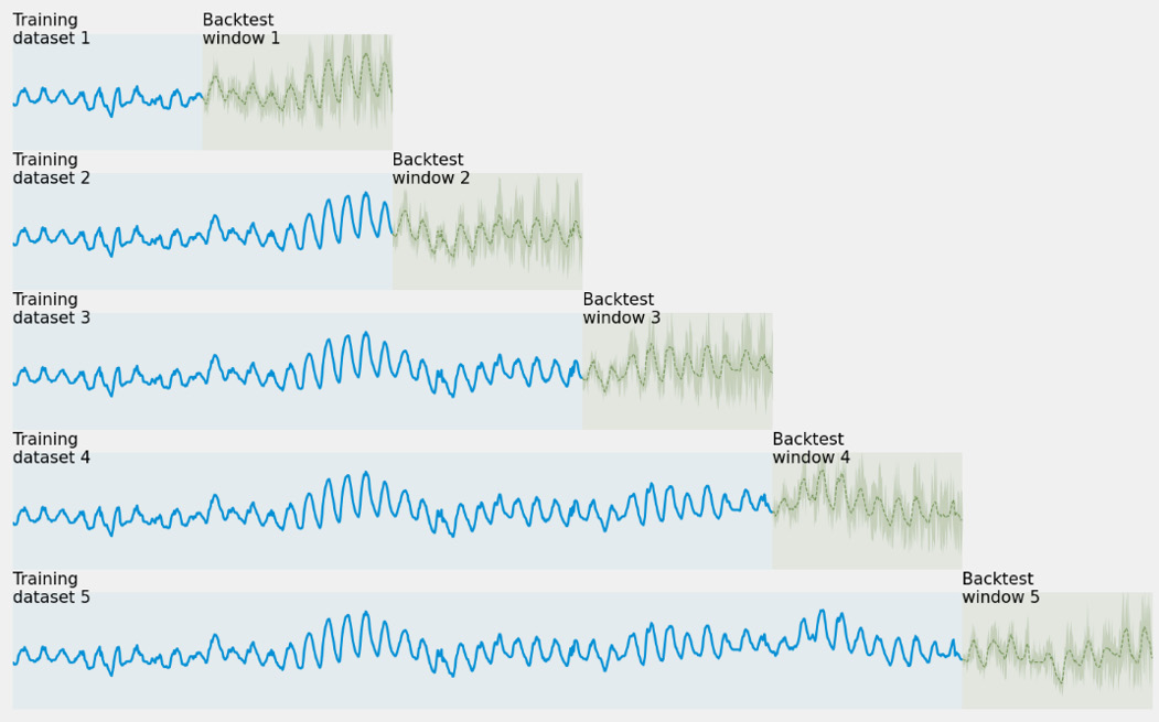
Figure 5.9 – Multiple backtest windows strategy

In the previous screenshot, you can see what Amazon Forecast will do when you select five backtest windows that have the same length as the forecast horizon. This is essentially what happens:

• In the first scenario, the service will train the predictor on a small portion of the data and evaluate it in roughly the same time span.
• Then, each backtest scenario will extend the training dataset and train on additional data while evaluating on a backtest window further in the future (with the same window width).
• At the end of the process, Amazon Forecast will train a new model on the whole dataset so that it's ready to be used for inference and generate new forecasts (this will be described in the next chapter).

Configuring your backtesting strategy happens in the Predictor settings section when you wish to create a new predictor without using the AutoPredictor settings, as illustrated in the following screenshot:

Figure 5.10 – Backtesting configuration for a new predictor

After you make your algorithm selection, you can choose from the following options:

• Number of backtest windows: This number can range from 1 to 5.
• Backtest window offset: This is the width of the window. By default, it is equal to the forecast horizon and has the same unit.

Let's create a new predictor with the following parameters:

• Predictor name: london_energy_cnnqr_backtest
• Forecast horizon: 30 (days)
• Algorithm selection: Manual
• Algorithm: CNN-QR
• Number of backtest windows: 5
• Backtest window offset: 30

Leave all the other parameters at their default values and click Start to create a new predictor with these settings. After an hour or so of training, you can explore the accuracy metric of this new predictor, as illustrated in the following screenshot:

Figure 5.11 – Backtesting accuracy metrics

You will notice that Amazon Forecast computes the accuracy metrics for each backtest window and also gives you the average of these metrics over five windows. You may note some fluctuations of the metrics, depending on the backtest window: this can be a good indicator of the variability of your time series across different time ranges, and you may run some more thorough investigation of your data over these different periods to try to understand the causes of these fluctuations.

You now know how to customize your backtesting strategy to make your training more robust. We are now going to look at how you can customize the features of your dataset by adding features provided by Amazon Forecast (namely, holidays and weather data).

Including holiday and weather data

At the time of writing this book, Amazon Forecast includes two built-in datasets that are made available as engineered features that you can leverage as supplementary features: Holidays and the Weather index.

Enabling the Holidays feature

This supplementary feature includes a dataset of national holidays for 66 countries. You can enable this feature when you create a new predictor: on the predictor creation page, scroll down to the optional Supplementary features section and toggle on the Enable holidays button, as illustrated in the following screenshot:

Figure 5.12 – Enabling the Holidays supplementary feature

Once enabled, a drop-down list appears, to let you select the country for which you want to enable holidays. Note that you can only select one country: your whole dataset must pertain to this country. If you have several countries in your dataset and wish to take different holidays into account, you will have to split your dataset by country and train a predictor on each of them.

When this parameter is selected, Amazon Forecast will train a model with and without this parameter: the best configuration will be kept based on the performance metric of your model.

Enabling the Weather index

This supplementary feature includes 2 years of historical weather data and 2 weeks of future weather information for 7 regions covering the whole world, as follows:

• US (excluding Hawaii and Alaska), with latitude ranging from 24.6 to 50.0 and longitude between -126.0 and -66.4
• Canada, with latitude ranging from 41.0 to 75.0 and longitude from -142.0 and 52.0
• Europe, with latitude ranging from 34.8 to 71.8 and longitude from -12.6 to 44.8
• South America, with latitude ranging from -56.6 to 14.0 and longitude from -82.2 to -33.0
• Central America, with latitude ranging from 6.8 to 33.20 and longitude from -118.80 to -58.20
• Africa & Middle East, with latitude ranging from -35.60 to 43.40 and longitude from -18.8 to -58.20
• Asia Pacific, with latitude ranging from -47.8 to 55.0 and longitude from -67.0 to 180.60

To leverage weather data in Amazon Forecast, you need to perform the following actions:

• Ensure your dataset has data pertaining exclusively to one single region (for instance, all your data must be linked to locations that are all in Europe). If you have several regions in your data, you will have to create a dataset per region and train one predictor per region.
• Add geolocation information to your dataset.
• Include a geolocation attribute when creating and ingesting your target dataset.
• Select AutoPredictor or AutoML when creating your predictor or manually select an algorithm.

Adding geolocation information to your dataset

Once you have a dataset with data from a single region (US, Canada, Europe, Central America, Africa & Middle East, or South America), you must add a location feature to your dataset. This feature can be one of the following:

• A ZIP code (if your locations are in the United States (US)). The column must follow this format: US, followed by an underscore character (_), followed by the 5-digit ZIP code. For instance, US_98121 is a valid postal code to be used.
• Latitude and longitude coordinates in decimal format, both coordinates being separated by an underscore character (_)—for instance, 47.61_-122.33 is a valid string. Amazon Forecast takes care of rounding to the nearest 0.2 degrees if you input raw values with more precision. This format is available for every region.

Our household electricity consumption dataset is from London and the coordinates of London are respectively 51.5073509 (latitude) and -0.1277583 (longitude). If we wanted to add weather data to our dataset, we could add a column called location to our dataset and set its value to 51.5073509_-0.1277583 for every row (as all our households are located in this city).

Important Tip

As mentioned previously, the Weather index is only available for the past 2 years. If you want to get some practice with this feature, make sure the availability of weather data is compatible with the recording time of your time series data. If your time series data includes data points before July 1, 2018, the weather_index parameter will be disabled in the user interface (UI).

Including a geolocation attribute

When ingesting a target time series data into a dataset group, you will have the opportunity to select a location type attribute. Follow these next steps:

1. After signing in to the AWS Management Console, open the Amazon Forecast console and click on the View dataset group button.
2. On the dataset group list screen presented to you, select an empty dataset group (or create a brand new one: you can refer back to Chapter 3, Creating a Project and Ingesting your Data, in case you need some guidance to create and configure a new dataset group).
3. When you're on your dataset group dashboard, click on the Import button that is next to the Target time series data label. You will arrive at the data ingestion wizard.
4. In the Schema Builder section, click on Add attribute, name your attribute location, and select geolocation for the Attribute Type value, as follows:

Figure 5.13 – Ingesting data with location information

5. For the Geolocation format option, you have a choice between Lat/Long Decimal Degrees or Postal Code (if your location data is in the US).

You can then continue with the ingestion process, as explained in Chapter 3, Creating a Project and Ingesting your Data. If you have other datasets, you can also ingest them in the related time series data and item metadata dataset. You can then train a new predictor based on this dataset group.

Creating a predictor with the Weather index

Once you have a dataset group with location data, you can enable the Weather index feature while creating a new predictor based on this dataset, as follows:

1. On the Amazon Forecast console, click on View dataset groups to bring up a list of existing dataset groups and choose a dataset group where your location-aware dataset has been ingested.
2. In the navigation pane, choose Predictors and click on Train new predictor.
3. On the predictor creation page, scroll down to the optional Supplementary features section and toggle on the Enable weather index button, as illustrated in the following screenshot:

Figure 5.14 – Enabling the Weather supplementary feature

When you're ready to train a predictor, click on the Create button at the bottom of the prediction creation screen to start training a predictor with weather data.

When this parameter is selected, Amazon Forecast will train a model with and without this parameter: the best configuration for each time series will be kept based on the performance metric of your model. In other words, if supplementing weather data to a given time series does not improve accuracy during backtesting, Amazon Forecast will disable the weather feature for this particular time series.

You have now a good idea of how to take weather data and holiday data into account in your forecasting strategy. In the next chapter, you are going to see how you can ask Amazon Forecast to preprocess the features you provide in your own dataset.

Implementing featurization techniques

Amazon Forecast lets you customize the way you can transform the input datasets by filling in missing values. The presence of missing values in raw data is very common and has a deep impact on the quality of your forecasting model. Indeed, each time a value is missing in your target or related time series data, the true observation is not available to assess the real distribution of historical data.

Although there can be multiple reasons why values are missing, the featurization pipeline offered by Amazon Forecast assumes that you are not able to fill in the values based on your domain expertise and that missing values are actually present in the raw data you ingested into the service. For instance, if we plot the energy consumption of the household with the identifier (ID) MAC002200, we can see that some values are missing at the end of the dataset, as shown in the following screenshot:

Figure 5.15 – Missing values for the energy consumption of the MAC002200 household

As we are dealing with the energy consumption of a household, this behavior is probably linked to a household that left this particular house. Let's see how you can configure the behavior of Amazon Forecast to deal with this type of situation.

Configuring featurization parameters

Configuring how to deal with missing values happens in the Advanced configuration settings of the Predictor details section when you wish to create a new predictor.

After logging in to the AWS console, navigate to the Amazon Forecast console and click on the View dataset groups button. There, you can click on the name of the dataset group you created in Chapter 3, Creating a Project and Ingesting your Data. You should now be on the dashboard of your dataset group, where you can click on Train predictor. Scroll to the bottom of the Predictor details section and click on Advanced configurations to unfold additional configurations. In this section, you will find the Hyperparameter optimization configuration, the Training parameter configuration (when available for the selected algorithm), and the Featurizations section, as illustrated in the following screenshot:

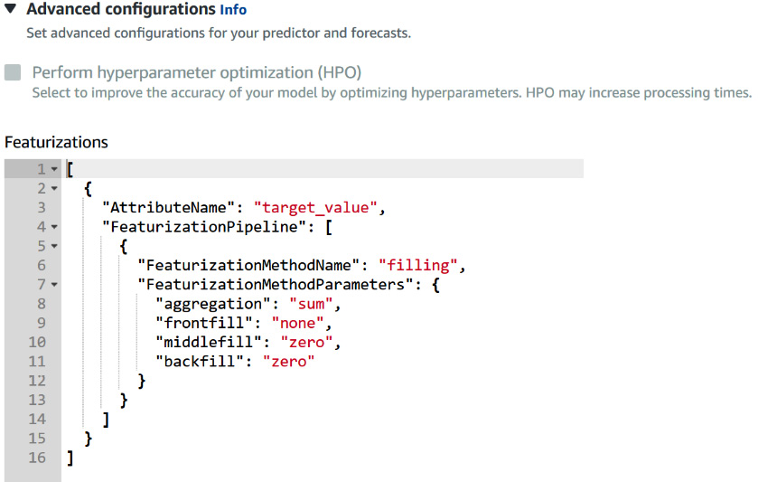
Figure 5.16 – Featurization configuration

The featurization is configured with this small JSON snippet, and you will have a similar section for every attribute you want to fill in missing values for.

By default, Amazon Forecast only fills in missing values in the target time series data and does not apply any transformation to the related time series data. There are three parameters you can configure, as follows:

• AttributeName: This can be either the target field of your target time series data or one of the fields of your related time series data. Depending on the domain selected, this can be demand, target_value, workforce_demand, value, metric_value, or number_of_instances. You can refer back to the schema of your target and related datasets to find which values you can use. In the energy consumption case you have been running, you initially selected the custom domain: the target field for this domain is target_value.
• FeaturizationMethodName: At the time of writing this book, only the filling method is available. The only value this field can take is filling.
• FeaturizationMethodParameters: For the filling method, there are two parameters you can configure for both related and target time series (middlefill and backfill). For the target time series, the frontfill parameter is set to none, and you can also specify an aggregation parameter. For the related time series, you can also specify the filling behavior to apply within the forecast horizon with the futurefill parameter.

The following screenshot illustrates these different handling strategies Amazon Forecast can leverage for filling missing values:

Figure 5.17 – Missing values handling strategies

The global start date is the earliest start date of all the items (illustrated in the preceding screenshot by the top two lines) present in your dataset, while the global end date is the last end date of all the items augmented by the forecast horizon.

Introducing featurization parameter values

The following table illustrates the possible values these parameters can take, depending on the dataset:

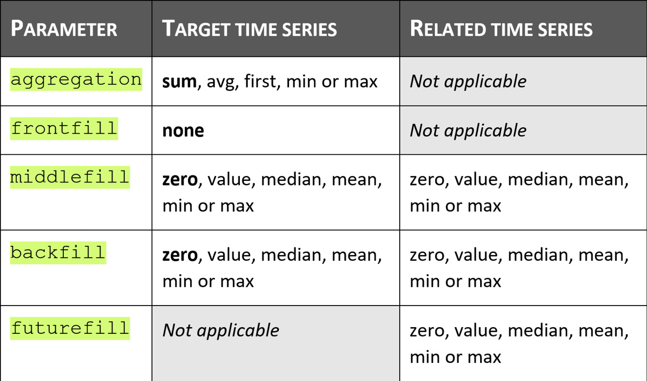
Figure 5.18 – Parameters and their possible values

Let's have a look at these parameters in more detail, as follows:

• aggregation: When the forecast frequency requested to create a predictor is different than the raw frequency of your dataset, Amazon Forecast will apply this parameter. By default, it aggregates your raw data by summing the values (sum). If your raw data was available at an hourly level and you request a predictor at the daily level, it will sum all the hourly data available to build a daily dataset. You have the option to alter this behavior by requesting Amazon Forecast to replace the sum by the average (avg), by taking the first value available (first) or by taking the minimum (min) or maximum (max) value over each considered period.
• Filling parameters: When applicable, the different filling behaviors available are zero (replace every missing value by zeros), value (replace by a given value), median (replace by the median of the whole time series), mean (replace by the mean), min, or max (replace by the minimum or maximum value of the whole time series).

There are no default values when applying filling methods to related time series (as you can have several series with different expected behavior). Values in bold in the preceding table are the default values applied to the target time series dataset.

When you select a value for one of the filling parameters, you have to define the desired value as a real value with an additional parameter obtained by adding _value to the name of the parameter, as follows:

• middlefill_value defines the replacement value when you select middlefill = value.
• backfill_value defines the replacement value when you select backfill = value.
• futurefill_value defines the replacement value when you select futurefill = value.

In this section, you discovered how you can rely on Amazon Forecast to preprocess your features and maintain the consistent data quality necessary to deliver robust and accurate forecasts. In the next section, you are going to dive deeper into how you can put the probabilistic aspect of Amazon Forecast to work to suit your own business needs.

Customizing quantiles to suit your business needs

Amazon Forecast generates probabilistic forecasts at different quantiles, giving you prediction intervals over mere point forecasts. Prediction quantiles (or intervals) let Amazon Forecast express the uncertainty of each prediction and give you more information to include in the decision-making process that is linked to your forecast exercise.

As you have seen earlier in this chapter, Amazon Forecast can leverage different forecasting algorithms: each of these algorithms has a different way to estimate probability distributions. For more details about the theoretical background behind probabilistic forecasting, you can refer to the following papers:

• GluonTS: Probabilistic Time Series Models in Python (https://arxiv.org/pdf/1906.05264.pdf), which gives you some details about the way the ARIMA, ETS, NPTS, and DeepAR+ algorithms generate these predictions' intervals.
• A Multi-Horizon Quantile Recurrent Forecaster (https://arxiv.org/pdf/1711.11053.pdf) gives details about how the neural quantile family of models (which include similar architectures to CNN-QR) generates these distributions while directly predicting given timesteps in the forecast horizon.
• The Prophet algorithm is described in detail in the original paper from Facebook and can be found here: https://peerj.com/preprints/3190/.

Let's now see how you can configure different forecast types when creating a new predictor.

Configuring your forecast types

Configuring the forecast types you want Amazon Forecast to generate happens on the Predictor details section when you wish to create a new predictor. By default, the quantiles selected are 10% (p10), 50% (the median, p50) and 90% (p90). When configuring a predictor, the desired quantiles are called forecast type and you can choose up to five of them, including any percentile ranging from 0.01 to 0.99 (with an increment of 0.01). You can also select mean as a forecast type.

Important Note

CNN-QR cannot generate a mean forecast, as this type of algorithm directly generates predictions for a particular quantile: when selecting mean as a forecast type, CNN-QR will fall back to computing the median (p50).

In the following screenshot, I configured my forecast types to request Amazon Forecast to generate the mean forecast and three quantiles (p10, p50, and p99):

Figure 5.19 – Selecting forecast types to generate

You can click on Remove to remove a forecast and request up to five forecast types by clicking on the Add new forecast type button.

Important Note

Amazon Forecast bills you for each time series forecast is generated: each forecast type counts for a billed item and they will always bill you for a minimum of three quantiles, even if you only intend to use one. It is hence highly recommended to customize the default quantiles to suit your business needs and benefit from the probabilistic capability of Amazon Forecast.

Amazon Forecast will compute a quantile loss metric for each requested quantile. In the following screenshot, you can see the default wQL metrics computed for the default quantiles generated by the service: wQL[0.1] is the quantile loss for the p10 forecast type, wQL[0.5] is for the median, and so on:

Figure 5.20 – Quantile loss metrics per forecast type

Let's now see how to choose the right quantiles depending on the type of decision you are expecting to make based on these predictions.

Choosing forecast types

Choosing a forecast type to suit your business need is a trade-off between the cost of over-forecasting (generating higher capital cost or higher inventory) and the cost of under-forecasting (missing revenue because a product is not available when a customer wishes to order it, or because you cannot produce finished goods to meet the actual market demand).

In Chapter 4, Training a Predictor with AutoML, you met the weighted quantile loss (wQL) metric. As a reminder, computing this metric for a given quantile can be done with the following formula:

Here, the following applies:

• is the actual value observed for a given item_id parameter at a point in time t (with t ranging over the time range from the backtest period and i ranging over all items).
• is the t quantile predicted for a given item_id parameter at a point in time t.
• is a quantile that can take of one the following values: 0.01, 0.02…, 0.98, or 0.99.

If you are building a sound vaccine strategy and want to achieve global immunity as fast as possible, you must meet your population demand at all costs (meaning that doses must be available when someone comes to get their shot). To meet such imperative demand, a p99 forecast may be very useful: this forecast type expects the true value to be lower than the predicted value 99% of the time. If we use = 0.99 in the previous formula, we end up with the following:

• A larger penalty weight to under-forecasting:
• A smaller penalty weight to over-forecasting:

Let's have a look at another example, as follows:

• If you own a garment store, you don't want to be out of stock of winter articles in winter: the capital cost of overstocking is cheaper (less chance to have many products stuck in your inventory) and a p90 forecast is useful to prevent you from running out of stock.
• On the other hand, when summer comes, you may take your stock decision for winter garments based on the p10 forecast (someone may buy this warm scarf, but there is a high probability that it may stay longer in your inventory before this happens).

As you can see, combining different forecast types gives you the ability to adjust your strategy depending on fluctuations over the year.

Summary

In this chapter, you discovered the many possibilities Amazon Forecast gives you to customize your predictor training to your datasets. You learned how to choose the best algorithm to fit your problem and how to customize different parameters (quantiles, the missing values' filling strategy, and supplementary features usage) to try to improve your forecasting models.

The AutoML capability of Amazon Forecast is a key differentiator when dealing with a new business case or a new dataset. It gives you good directions and reliable results with a fast turnaround. However, achieving higher accuracy to meet your business needs means that you must sometimes be able to override Amazon Forecast decisions by orienting its choice of algorithms, deciding how to process the features of your dataset, or simply requesting a different set of outputs by selecting forecast types that match the way your decision process is run from a business perspective.

In the next chapter, you will use a trained predictor to generate new forecasts (in ML terms, we will use new data to run inferences on a trained model).