9

Generative Models

Generative models are a type of machine learning algorithm that is used to create data. They are used to generate new data that is similar to the data that was used to train the model. They can be used to create new data for testing or to fill in missing data. Generative models are used in many applications, such as density estimation, image synthesis, and natural language processing. The VAE discussed in Chapter 8, Autoencoders, was one type of generative model; in this chapter, we will discuss a wide range of generative models, Generative Adversarial Networks (GANs) and their variants, flow-based models, and diffusion models.

GANs have been defined as the most interesting idea in the last 10 years in ML (https://www.quora.com/What-are-some-recent-and-potentially-upcoming-breakthroughs-in-deep-learning) by Yann LeCun, one of the fathers of deep learning. GANs are able to learn how to reproduce synthetic data that looks real. For instance, computers can learn how to paint and create realistic images. The idea was originally proposed by Ian Goodfellow (for more information, refer to NIPS 2016 Tutorial: Generative Adversarial Networks, by I. Goodfellow, 2016); he has worked with the University of Montreal, Google Brain, and OpenAI, and is presently working in Apple Inc. as the Director of Machine Learning.

In this chapter, we will cover different types of GANs; the chapter will introduce you to flow-based models and diffusion models, and additionally, you will see some of their implementation in TensorFlow. Broadly, we will cover the following topics:

• What is a GAN?
• Deep convolutional GANs
• InfoGAN
• SRGAN
• CycleGAN
• Applications of GANs
• Flow-based generative models
• Diffusion models for data generation

Let’s begin!

What is a GAN?

The ability of GANs to learn high-dimensional, complex data distributions has made them very popular with researchers in recent years. Between 2016, when they were first proposed by Ian Goodfellow, to March 2022, we have more than 100,000 research papers related to GANs, just in the space of 6 years!

The applications of GANs include creating images, videos, music, and even natural languages. They have been employed in tasks like image-to-image translation, image super-resolution, drug discovery, and even next-frame prediction in video. They have been especially successful in the task of synthetic data generation – both for training the deep learning models and assessing the adversarial attacks.

The key idea of GAN can be easily understood by considering it analogous to “art forgery,” which is the process of creating works of art that are falsely credited to other usually more famous artists. GANs train two neural nets simultaneously. The generator G(Z) is the one that makes the forgery, and the discriminator D(Y) is the one that can judge how realistic the reproductions are, based on its observations of authentic pieces of art and copies. D(Y) takes an input Y (for instance, an image), and expresses a vote to judge how real the input is. In general, a value close to 1 denotes “real,” while a value close to 0 denotes “forgery.” G(Z) takes an input from random noise Z and it trains itself to fool D into thinking that whatever G(Z) produces is real.

The goal of training the discriminator D(Y) is to maximize D(Y) for every image from the true data distribution and to minimize D(Y) for every image not from the true data distribution. So, G and D play opposite games, hence the name adversarial training. Note that we train G and D in an alternating manner, where each one of their objectives is expressed as a loss function optimized via a gradient descent. The generative model continues to improve its forgery capabilities, and the discriminative model continues to improve its forgery recognition capabilities. The discriminator network (usually a standard convolutional neural network) tries to classify if an input image is real or generated. The important new idea is to backpropagate through both the discriminator and the generator to adjust the generator’s parameters in such a way that the generator can learn how to fool the discriminator more often. In the end, the generator will learn how to produce images that are indistinguishable from the real ones:

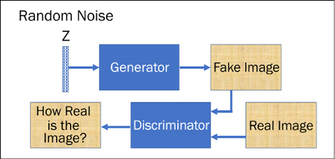
Figure 9.1: Basic architecture of a GAN

Of course, GANs involve working towards equilibrium in a game involving two players. Let us first understand what we mean by equilibrium here. When we start, one of the two players is hopefully better than the other. This pushes the other to improve and this way, both the generator and discriminator push each other towards improvement.

Eventually, we reach a state where the improvement is not significant in either player. We check this by plotting the loss function, to see when the two losses (gradient loss and discriminator loss) reach a plateau. We don’t want the game to be skewed too heavily one way; if the forger were to immediately learn how to fool the judge on every occasion, then the forger has nothing more to learn. Practically training GANs is really hard, and a lot of research is being done in analyzing GAN convergence; check this site: https://avg.is.tuebingen.mpg.de/projects/convergence-and-stability-of-gan-training for details on convergence and stability of different types of GANs. In generative applications of GAN, we want the generator to learn a little better than the discriminator.

Let’s now delve deep into how GANs learn. Both the discriminator and generator take turns to learn. The learning can be divided into two steps:

1. Here the discriminator, D(x), learns. The generator, G(z), is used to generate fake images from random noise z (which follows some prior distribution P(z)). The fake images from the generator and the real images from the training dataset are both fed to the discriminator, and it performs supervised learning trying to separate fake from real. If P_data (x) is the training dataset distribution, then the discriminator network tries to maximize its objective so that D(x) is close to 1 when the input data is real and close to zero when the input data is fake.
2. In the next step, the generator network learns. Its goal is to fool the discriminator network into thinking that generated G(z) is real, that is, force D(G(z)) close to 1.

The two steps are repeated sequentially. Once the training ends, the discriminator is no longer able to discriminate between real and fake data and the generator becomes a pro in creating data very similar to the training data. The stability between discriminator and generator is an actively researched problem.

Now that you have got an idea of what GANs are, let’s look at a practical application of a GAN in which “handwritten” digits are generated.

MNIST using GAN in TensorFlow

Let us build a simple GAN capable of generating handwritten digits. We will use the MNIST handwritten digits to train the network. We will need to import TensorFlow modules; to keep the code clean, we export all the classes that we will require from the TensorFlow framework:

from tensorflow.keras.datasets import mnist
from tensorflow.keras.layers import Input, Dense, Reshape, Flatten, Dropout
from tensorflow.keras.layers import BatchNormalization, Activation, ZeroPadding2D
from tensorflow.keras.layers import LeakyReLU
from tensorflow.keras.layers import UpSampling2D, Conv2D
from tensorflow.keras.models import Sequential, Model
from tensorflow.keras.optimizers import Adam
from tensorflow.keras import initializers
import matplotlib.pyplot as plt
import numpy as np

We use the TensorFlow Keras dataset to access the MNIST data. The data contains 60,000 training images of handwritten digits each of size 28 × 28. The pixel value of the digits lies between 0-255; we normalize the input values such that each pixel has a value in the range [-1, 1]:

randomDim = 10
(X_train, _), (_,  _) = mnist.load_data()
X_train = (X_train.astype(np.float32) - 127.5)/127.5

We will use a simple multi-layered perceptron (MLP) and we will feed it an image as a flat vector of size 784, so we reshape the training data:

X_train = X_train.reshape(60000, 784)

Now we will need to build a generator and discriminator. The purpose of the generator is to take in a noisy input and generate an image similar to the training dataset. The size of the noisy input is decided by the variable randomDim; you can initialize it to any integral value. Conventionally, people set it to 100. For our implementation, we tried a value of 10. This input is fed to a dense layer with 256 neurons with LeakyReLU activation. We next add another dense layer with 512 hidden neurons, followed by the third hidden layer with 1024 neurons, and finally the output layer with 784 neurons. You can change the number of neurons in the hidden layers and see how the performance changes; however, the number of neurons in the output unit has to match the number of pixels in the training images. The corresponding generator is then:

generator = Sequential()
generator.add(Dense(256, input_dim=randomDim))
generator.add(LeakyReLU(0.2))
generator.add(Dense(512))
generator.add(LeakyReLU(0.2))
generator.add(Dense(1024))
generator.add(LeakyReLU(0.2))
generator.add(Dense(784, activation='tanh'))

Similarly, we build a discriminator. Notice now (Figure 9.1) that the discriminator takes in the images, either from the training set or images generated by the generator, thus its input size is 784. Additionally, here we are using a TensorFlow initializer to initialize the weights of the dense layer, we are using a normal distribution with a standard deviation of 0.02 and a mean of 0. As mentioned in Chapter 1, Neural Network Foundations with TF, there are many initializers available in the TensorFlow framework. The output of the discriminator is a single bit, with 0 signifying a fake image (generated by generator) and 1 signifying that the image is from the training dataset:

discriminator = Sequential()
discriminator.add(Dense(1024, input_dim=784, kernel_initializer=initializers.RandomNormal(stddev=0.02))
)
discriminator.add(LeakyReLU(0.2))
discriminator.add(Dropout(0.3))
discriminator.add(Dense(512))
discriminator.add(LeakyReLU(0.2))
discriminator.add(Dropout(0.3))
discriminator.add(Dense(256))
discriminator.add(LeakyReLU(0.2))
discriminator.add(Dropout(0.3))
discriminator.add(Dense(1, activation='sigmoid'))

Next, we combine the generator and discriminator together to form a GAN. In the GAN, we ensure that the discriminator weights are fixed by setting the trainable argument to False:

discriminator.trainable = False
ganInput = Input(shape=(randomDim,))
x = generator(ganInput)
ganOutput = discriminator(x)
gan = Model(inputs=ganInput, outputs=ganOutput)

The trick to training the two is that we first train the discriminator separately; we use binary cross-entropy loss for the discriminator. Later, we freeze the weights of the discriminator and train the combined GAN; this results in the training of the generator. The loss this time is also binary cross-entropy:

discriminator.compile(loss='binary_crossentropy', optimizer='adam')
gan.compile(loss='binary_crossentropy', optimizer='adam')

Let us now perform the training. For each epoch, we take a sample of random noise first, feed it to the generator, and the generator produces a fake image. We combine the generated fake images and the actual training images in a batch with their specific labels and use them to train the discriminator first on the given batch:

def train(epochs=1, batchSize=128):
    batchCount = int(X_train.shape[0] / batchSize)
    print ('Epochs:', epochs)
    print ('Batch size:', batchSize)
    print ('Batches per epoch:', batchCount)
    for e in range(1, epochs+1):
        print ('-'*15, 'Epoch %d' % e, '-'*15)
        for _ in range(batchCount):
            # Get a random set of input noise and images
            noise = np.random.normal(0, 1, size=[batchSize,
            randomDim])
            imageBatch = X_train[np.random.randint(0,
            X_train.shape[0], size=batchSize)]
            # Generate fake MNIST images
            generatedImages = generator.predict(noise)
            # print np.shape(imageBatch), np.shape(generatedImages)
            X = np.concatenate([imageBatch, generatedImages])
            # Labels for generated and real data
            yDis = np.zeros(2*batchSize)
            # One-sided label smoothing
            yDis[:batchSize] = 0.9
            # Train discriminator
            discriminator.trainable = True
            dloss = discriminator.train_on_batch(X, yDis)

If you notice, while assigning labels, instead of 0/1 we used 0/0.9 – this is called label smoothing. It has been found that keeping a soft target improves both generalization and learning speed (When does label smoothing help?, Muller et al. NeurIPS 2019).

Now, in the same for loop, we will train the generator. We want the images generated by the generator to be detected as real by the discriminator, so we use a random vector (noise) as input to the generator; this generates a fake image and then trains the GAN such that the discriminator perceives the image as real (the output is 1):

            # Train generator
            noise = np.random.normal(0, 1, size=[batchSize,
            randomDim])
            yGen = np.ones(batchSize)
            discriminator.trainable = False
            gloss = gan.train_on_batch(noise, yGen)

Cool trick, right? If you wish to, you can save the generator and discriminator loss as well as the generated images. Next, we are saving the losses for each epoch and generating images after every 20 epochs:

        # Store loss of most recent batch from this epoch
        dLosses.append(dloss)
        gLosses.append(gloss)
        if e == 1 or e % 20 == 0:
               saveGeneratedImages(e)

We can now train the GAN by calling the train function. In the following graph, you can see the plot of both generative and discriminative loss as the GAN is learning:

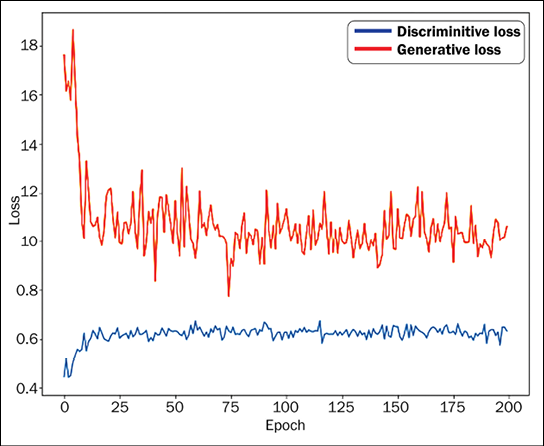
Figure 9.2: Discriminator and generator loss plots

And handwritten digits generated by our GAN:

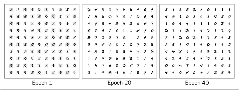
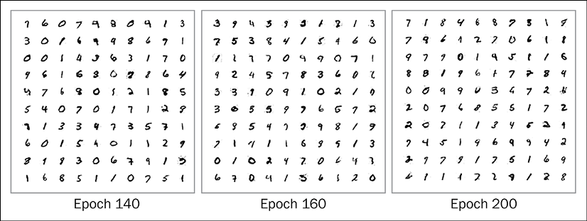
Figure 9.3: Generated handwritten digits

You can see from the preceding figures that as the epochs increase, the handwritten digits generated by the GAN become more and more realistic.

To plot the loss and the generated images of the handwritten digits, we define two helper functions, plotLoss() and saveGeneratedImages(). Their code is given as follows:

# Plot the loss from each batch
def plotLoss(epoch):
    plt.figure(figsize=(10, 8))
    plt.plot(dLosses, label='Discriminitive loss')
    plt.plot(gLosses, label='Generative loss')
    plt.xlabel('Epoch')
    plt.ylabel('Loss')
    plt.legend()
    plt.savefig('images/gan_loss_epoch_%d.png' % epoch)
# Create a wall of generated MNIST images
def saveGeneratedImages(epoch, examples=100, dim=(10, 10), figsize=(10, 10)):
    noise = np.random.normal(0, 1, size=[examples, randomDim])
    generatedImages = generator.predict(noise)
    generatedImages = generatedImages.reshape(examples, 28, 28)
    plt.figure(figsize=figsize)
    for i in range(generatedImages.shape[0]):
        plt.subplot(dim[0], dim[1], i+1)
        plt.imshow(generatedImages[i], interpolation='nearest',
        cmap='gray_r')
        plt.axis('off')
    plt.tight_layout()
    plt.savefig('images/gan_generated_image_epoch_%d.png' % epoch)

The saveGeneratedImages function saves images in the images folder, so make sure you have created the folder in your current working directory. The complete code for this can be found in the notebook VanillaGAN.ipynb at the GitHub repo for this chapter. In the coming sections, we will cover some recent GAN architectures and implement them in TensorFlow.

Deep convolutional GAN (DCGAN)

Proposed in 2016, DCGANs have become one of the most popular and successful GAN architectures. The main idea of the design was using convolutional layers without the use of pooling layers or the end classifier layers. The convolutional strides and transposed convolutions are employed for the downsampling (the reduction of dimensions) and upsampling (the increase of dimensions. In GANs, we do this with the help of a transposed convolution layer. To know more about transposed convolution layers, refer to the paper A guide to convolution arithmetic for deep learning by Dumoulin and Visin) of images.

Before going into the details of the DCGAN architecture and its capabilities, let us point out the major changes that were introduced in the paper:

• The network consisted of all convolutional layers. The pooling layers were replaced by strided convolutions (i.e., instead of one single stride while using the convolutional layer, we increased the number of strides to two) in the discriminator and transposed convolutions in the generator.
• The fully connected classifying layers after the convolutions are removed.
• To help with the gradient flow, batch normalization is done after every convolutional layer.

The basic idea of DCGANs is the same as the vanilla GAN: we have a generator that takes in noise of 100 dimensions; the noise is projected and reshaped, and is then passed through convolutional layers. Figure 9.4 shows the generator architecture:

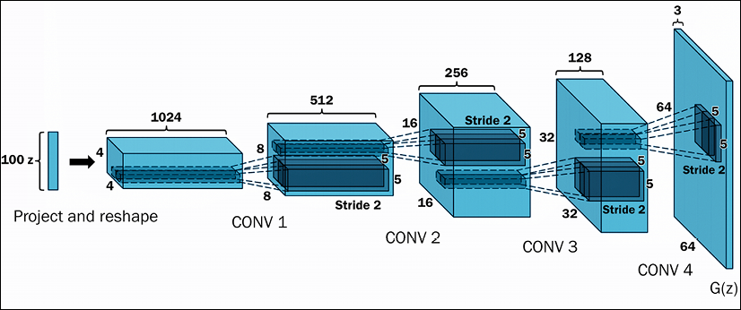
Figure 9.4: Visualizing the architecture of a generator

The discriminator network takes in the images (either generated by the generator or from the real dataset), and the images undergo convolution followed by batch normalization. At each convolution step, the images get downsampled using strides. The final output of the convolutional layer is flattened and feeds a one-neuron classifier layer.

In Figure 9.5, you can see the discriminator:

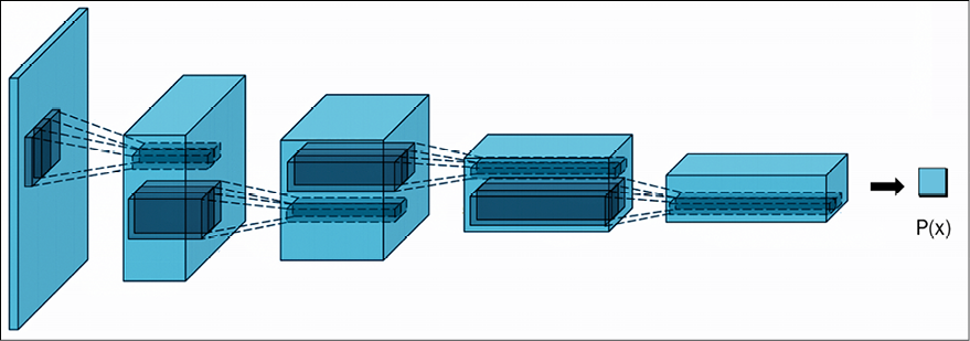
Figure 9.5: Visualizing the architecture of a discriminator

The generator and the discriminator are combined together to form the DCGAN. The training follows in the same manner as before; that is, we first train the discriminator on a mini-batch, then freeze the discriminator and train the generator. The process is repeated iteratively for a few thousand epochs. The authors found that we get more stable results with the Adam optimizer and a learning rate of 0.002.

Next, we’ll implement a DCGAN for generating handwritten digits.

DCGAN for MNIST digits

Let us now build a DCGAN for generating handwritten digits. We first see the code for the generator. The generator is built by adding the layers sequentially. The first layer is a dense layer that takes the noise of 100 dimensions as an input. The 100-dimensional input is expanded to a flat vector of size 128 × 7 × 7. This is done so that finally, we get an output of size 28 × 28, the standard size of MNIST handwritten digits. The vector is reshaped to a tensor of size 7 × 7 × 128. This vector is then upsampled using the TensorFlow Keras UpSampling2D layer. Please note that this layer simply scales up the image by doubling rows and columns. The layer has no weights, so it is computationally cheap.

The Upsampling2D layer will now double the rows and columns of the 7 × 7 × 128 (rows × columns × channels) image, yielding an output of size 14 × 14 × 128. The upsampled image is passed to a convolutional layer. This convolutional layer learns to fill in the details in the upsampled image. The output of a convolution is passed to batch normalization for better gradient flow. The batch normalized output then undergoes ReLU activation in all the intermediate layers. We repeat the structure, that is, upsampling | convolution | batch normalization | ReLU. In the following generator, we have two such structures, the first with 128 filters, and the second with 64 filters in the convolution operation. The final output is obtained from a pure convolutional layer with 3 filters and tan hyperbolic activation, yielding an image of size 28 × 28 × 1:

def build_generator(self):
    model = Sequential()
    model.add(Dense(128 * 7 * 7, activation="relu",
    input_dim=self.latent_dim))
    model.add(Reshape((7, 7, 128)))
    model.add(UpSampling2D())
    model.add(Conv2D(128, kernel_size=3, padding="same"))
    model.add(BatchNormalization(momentum=0.8))
    model.add(Activation("relu"))
    model.add(UpSampling2D())
    model.add(Conv2D(64, kernel_size=3, padding="same"))
    model.add(BatchNormalization(momentum=0.8))
    model.add(Activation("relu"))
    model.add(Conv2D(self.channels, kernel_size=3, padding="same"))
    model.add(Activation("tanh"))
    model.summary()
    noise = Input(shape=(self.latent_dim,))
    img = model(noise)
    return Model(noise, img)

The resultant generator model is as follows:

Model: "sequential_1"
_________________________________________________________________
 Layer (type)                Output Shape              Param #   
=================================================================
 conv2d_3 (Conv2D)           (None, 14, 14, 32)        320       
                                                                 
 leaky_re_lu (LeakyReLU)     (None, 14, 14, 32)        0         
                                                                 
 dropout (Dropout)           (None, 14, 14, 32)        0         
                                                                 
 conv2d_4 (Conv2D)           (None, 7, 7, 64)          18496     
                                                                 
 zero_padding2d (ZeroPadding  (None, 8, 8, 64)         0         
 2D)                                                             
                                                                 
 batch_normalization_2 (Batc  (None, 8, 8, 64)         256       
 hNormalization)                                                 
                                                                 
 leaky_re_lu_1 (LeakyReLU)   (None, 8, 8, 64)          0         
                                                                 
 dropout_1 (Dropout)         (None, 8, 8, 64)          0         
                                                                 
 conv2d_5 (Conv2D)           (None, 4, 4, 128)         73856     
                                                                 
 batch_normalization_3 (Batc  (None, 4, 4, 128)        512       
 hNormalization)                                                 
                                                                 
 leaky_re_lu_2 (LeakyReLU)   (None, 4, 4, 128)         0         
                                                                 
 dropout_2 (Dropout)         (None, 4, 4, 128)         0         
                                                                 
 conv2d_6 (Conv2D)           (None, 4, 4, 256)         295168    
                                                                 
 batch_normalization_4 (Batc  (None, 4, 4, 256)        1024      
 hNormalization)                                                 
                                                                 
 leaky_re_lu_3 (LeakyReLU)   (None, 4, 4, 256)         0         
                                                                 
 dropout_3 (Dropout)         (None, 4, 4, 256)         0         
                                                                 
 flatten (Flatten)           (None, 4096)              0         
                                                                 
 dense_1 (Dense)             (None, 1)                 4097      
                                                                 
=================================================================
Total params: 393,729
Trainable params: 392,833
Non-trainable params: 896

You can also experiment with the transposed convolution layer. This layer not only upsamples the input image but also learns how to fill in details during the training. Thus, you can replace upsampling and convolution layers with a single transposed convolution layer. The transpose convolutional layer performs an inverse convolution operation. You can read about it in more detail in the paper: A guide to convolution arithmetic for deep learning (https://arxiv.org/abs/1603.07285).

Now that we have a generator, let us see the code to build the discriminator. The discriminator is similar to a standard convolutional neural network but with one major change: instead of max pooling, we use convolutional layers with strides of 2. We also add dropout layers to avoid overfitting, and batch normalization for better accuracy and fast convergence. The activation layer is leaky ReLU. In the following network, we use three such convolutional layers, with filters of 32, 64, and 128 respectively. The output of the third convolutional layer is flattened and fed to a dense layer with a single unit.

The output of this unit classifies the image as fake or real:

def build_discriminator(self):
    model = Sequential()
    model.add(Conv2D(32, kernel_size=3, strides=2,
    input_shape=self.img_shape, padding="same"))
    model.add(LeakyReLU(alpha=0.2))
    model.add(Dropout(0.25))
    model.add(Conv2D(64, kernel_size=3, strides=2, padding="same"))
    model.add(ZeroPadding2D(padding=((0,1),(0,1))))
    model.add(BatchNormalization(momentum=0.8))
    model.add(LeakyReLU(alpha=0.2))
    model.add(Dropout(0.25))
    model.add(Conv2D(128, kernel_size=3, strides=2, padding="same"))
    model.add(BatchNormalization(momentum=0.8))
    model.add(LeakyReLU(alpha=0.2))
    model.add(Dropout(0.25))
    model.add(Conv2D(256, kernel_size=3, strides=1, padding="same"))
    model.add(BatchNormalization(momentum=0.8))
    model.add(LeakyReLU(alpha=0.2))
    model.add(Dropout(0.25))
    model.add(Flatten())
    model.add(Dense(1, activation='sigmoid'))
    model.summary()
    img = Input(shape=self.img_shape)
    validity = model(img)
    return Model(img, validity)

The resultant discriminator network is:

Model: "sequential"
_________________________________________________________________
 Layer (type)                Output Shape              Param #   
=================================================================
 dense (Dense)               (None, 6272)              633472    
                                                                 
 reshape (Reshape)           (None, 7, 7, 128)         0         
                                                                 
 up_sampling2d (UpSampling2D  (None, 14, 14, 128)      0         
 )                                                               
                                                                 
 conv2d (Conv2D)             (None, 14, 14, 128)       147584    
                                                                 
 batch_normalization (BatchN  (None, 14, 14, 128)      512       
 ormalization)                                                   
                                                                 
 activation (Activation)     (None, 14, 14, 128)       0         
                                                                 
 up_sampling2d_1 (UpSampling  (None, 28, 28, 128)      0         
 2D)                                                             
                                                                 
 conv2d_1 (Conv2D)           (None, 28, 28, 64)        73792     
                                                                 
 batch_normalization_1 (Batc  (None, 28, 28, 64)       256       
 hNormalization)                                                 
                                                                 
 activation_1 (Activation)   (None, 28, 28, 64)        0         
                                                                 
 conv2d_2 (Conv2D)           (None, 28, 28, 1)         577       
                                                                 
 activation_2 (Activation)   (None, 28, 28, 1)         0         
                                                                 
=================================================================
Total params: 856,193
Trainable params: 855,809
Non-trainable params: 384
_________________________________________________________________

The complete GAN is made by combining the two:

class DCGAN():
    def __init__(self, rows, cols, channels, z = 10):
        # Input shape
        self.img_rows = rows
        self.img_cols = cols
        self.channels = channels
        self.img_shape = (self.img_rows, self.img_cols, self.channels)
        self.latent_dim = z
        optimizer = Adam(0.0002, 0.5)
        # Build and compile the discriminator
        self.discriminator = self.build_discriminator()
        self.discriminator.compile(loss=’binary_crossentropy’,
            optimizer=optimizer,
            metrics=[‘accuracy’])
        # Build the generator
        self.generator = self.build_generator()
        # The generator takes noise as input and generates imgs
        z = Input(shape=(self.latent_dim,))
        img = self.generator(z)
        # For the combined model we will only train the generator
        self.discriminator.trainable = False
        # The discriminator takes generated images as input and determines validity
        valid = self.discriminator(img)
        # The combined model  (stacked generator and discriminator)
        # Trains the generator to fool the discriminator
        self.combined = Model(z, valid)
        self.combined.compile(loss=’binary_crossentropy’, optimizer=optimizer)

As you might have noticed, we are defining here the binary_crossentropy loss object, which we will use later to define the generator and discriminator losses. Optimizers for both the generator and discriminator is defined in this init method. And finally, we define a TensorFlow checkpoint that we will use to save the two models (generator and discriminator) as the model trains.

The GAN is trained in the same manner as before; at each step, first, random noise is fed to the generator. The output of the generator is added with real images to initially train the discriminator, and then the generator is trained to give an image that can fool the discriminator.

The process is repeated for the next batch of images. The GAN takes between a few hundred to thousands of epochs to train:

   def train(self, epochs, batch_size=256, save_interval=50):
        # Load the dataset
        (X_train, _), (_, _) = mnist.load_data()
        # Rescale -1 to 1
        X_train = X_train / 127.5 - 1.
        X_train = np.expand_dims(X_train, axis=3)
        # Adversarial ground truths
        valid = np.ones((batch_size, 1))
        fake = np.zeros((batch_size, 1))
        for epoch in range(epochs):
            # ---------------------
            #  Train Discriminator
            # ---------------------
            # Select a random half of images
            idx = np.random.randint(0, X_train.shape[0], batch_size)
            imgs = X_train[idx]
            # Sample noise and generate a batch of new images
            noise = np.random.normal(0, 1, (batch_size, self.latent_dim))
            gen_imgs = self.generator.predict(noise)
            # Train the discriminator (real classified as ones and generated as zeros)
            d_loss_real = self.discriminator.train_on_batch(imgs, valid)
            d_loss_fake = self.discriminator.train_on_batch(gen_imgs, fake)
            d_loss = 0.5 * np.add(d_loss_real, d_loss_fake)
            # ---------------------
            #  Train Generator
            # ---------------------
            # Train the generator (wants discriminator to mistake images as real)
            g_loss = self.combined.train_on_batch(noise, valid)
            # Plot the progress
            print ("%d [D loss: %f, acc.: %.2f%%] [G loss: %f]" % (epoch, d_loss[0], 100*d_loss[1], g_loss))
            # If at save interval => save generated image samples
            if epoch % save_interval == 0:
                self.save_imgs(epoch)

Lastly, we need a helper function to save images:

    def save_imgs(self, epoch):
        r, c = 5, 5
        noise = np.random.normal(0, 1, (r * c, self.latent_dim))
        gen_imgs = self.generator.predict(noise)
        # Rescale images 0 - 1
        gen_imgs = 0.5 * gen_imgs + 0.5
        fig, axs = plt.subplots(r, c)
        cnt = 0
        for i in range(r):
            for j in range(c):
                axs[i,j].imshow(gen_imgs[cnt, :,:,0], cmap='gray')
                axs[i,j].axis('off')
                cnt += 1
        fig.savefig("images/dcgan_mnist_%d.png" % epoch)
        plt.close()

Let us now train our GAN:

dcgan = DCGAN(28,28,1)
dcgan.train(epochs=5000, batch_size=256, save_interval=50)

The images generated by our GAN as it learned to fake handwritten digits are:

Figure 9.6: Images generated by GAN – initial attempt

The preceding images were the initial attempts by the GAN. As it learned through the following 10 epochs, the quality of digits generated improved manyfold:

Figure 9.7: Images generated by GAN after 6, 8, and 10 epochs

The complete code is available in DCGAN.ipynb in the GitHub repo. We can take the concepts discussed here and apply them to images in other domains. One of the interesting works on images was reported in the paper, Unsupervised Representation Learning with Deep Convolutional Generative Adversarial Networks, Alec Radford, Luke Metz, Soumith Chintala, 2015. Quoting the abstract:

In recent years, supervised learning with convolutional networks (CNNs) has seen huge adoption in computer vision applications. Comparatively, unsupervised learning with CNNs has received less attention. In this work we hope to help bridge the gap between the success of CNNs for supervised learning and unsupervised learning. We introduce a class of CNNs called deep convolutional generative adversarial networks (DCGANs), that have certain architectural constraints, and demonstrate that they are a strong candidate for unsupervised learning. Training on various image datasets, we show convincing evidence that our deep convolutional adversarial pair learns a hierarchy of representations from object parts to scenes in both the generator and discriminator. Additionally, we use the learned features for novel tasks - demonstrating their applicability as general image representations.

—Radford et al., 2015

Following are some of the interesting results of applying DCGANs to a celebrity image dataset:

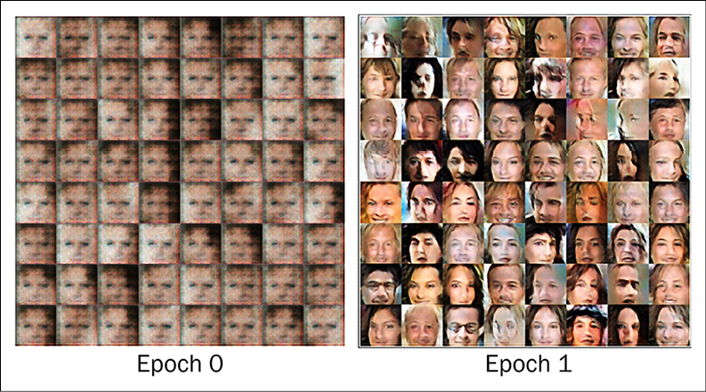
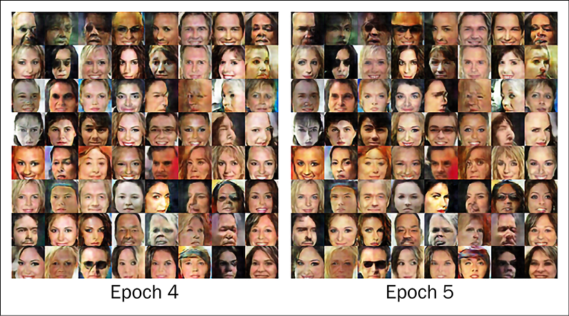
Figure 9.8: Generated celebrity images using DCGAN

Another interesting paper is Semantic Image Inpainting with Perceptual and Contextual Losses, by Raymond A. Yeh et al. in 2016. Just as content-aware fill is a tool used by photographers to fill in unwanted or missing parts of images, in this paper they used a DCGAN for image completion.

As mentioned earlier, a lot of research is happening around GANs. In the next section, we will explore some of the interesting GAN architectures proposed in recent years.

Some interesting GAN architectures

Since their inception, a lot of interest has been generated in GANs, and as a result, we are seeing a lot of modifications and experimentation with GAN training, architecture, and applications. In this section, we will explore some interesting GANs proposed in recent years.

SRGAN

Remember seeing a crime thriller where our hero asks the computer guy to magnify the faded image of the crime scene? With the zoom, we can see the criminal’s face in detail, including the weapon used and anything engraved upon it! Well, Super Resolution GANs (SRGANs) can perform similar magic. Magic in the sense that because GANs show that it is possible to get high-resolution images, the final results depend on the camera resolution used. Here, a GAN is trained in such a way that it can generate a photorealistic high-resolution image when given a low-resolution image. The SRGAN architecture consists of three neural networks: a very deep generator network (which uses Residual modules; see ResNets in Chapter 20, Advanced Convolutional Neural Networks), a discriminator network, and a pretrained VGG-16 network.

SRGANs use the perceptual loss function (developed by Johnson et al; you can find the link to the paper in the References section). In SRGAN, the authors first downsampled a high-resolution image and used the generator to get its “high-resolution” version. The discriminator was trained to differentiate between the real high-resolution image and the generated high-resolution image. The difference in the feature map activations in high layers of a VGG network between the network output and the high-resolution parts comprises the perceptual loss function. Besides perceptual loss, the authors further added content loss and an adversarial loss so that images generated look more natural and the finer details more artistic. The perceptual loss is defined as the weighted sum of the content loss and adversarial loss:

The first term on the right-hand side is the content loss, obtained using the feature maps generated by pretrained VGG 19. Mathematically, it is the Euclidean distance between the feature map of the reconstructed image (that is, the one generated by the generator) and the original high-resolution reference image. The second term on the RHS is the adversarial loss. It is the standard generative loss term, designed to ensure that images generated by the generator can fool the discriminator. You can see in the following figure that the image generated by the SRGAN is much closer to the original high-resolution image with a PSNR value of 37.61:

Figure 9.9: An example following the paper Photo-Realistic Single Image Super-Resolution Using a Generative Adversarial Network, Ledig et al.

Another noteworthy architecture is CycleGAN; proposed in 2017, it can perform the task of image translation. Once trained you can translate an image from one domain to another domain. For example, when trained on a horse and zebra dataset, if you give it an image with horses in the foreground, the CycleGAN can convert the horses to zebras with the same background. We will explore it next.

CycleGAN

Have you ever imagined how some scenery would look if Van Gogh or Manet had painted it? We have many scenes and landscapes painted by Van Gogh/Manet, but we do not have any collection of input-output pairs. A CycleGAN performs the image translation, that is, transfers an image given in one domain (scenery, for example) to another domain (a Van Gogh painting of the same scene, for instance) in the absence of training examples. The CycleGAN’s ability to perform image translation in the absence of training pairs is what makes it unique.

To achieve image translation, the authors used a very simple yet effective procedure. They made use of two GANs, the generator of each GAN performing the image translation from one domain to another.

To elaborate, let us say the input is X, then the generator of the first GAN performs a mapping ; thus, its output would be Y = G(X). The generator of the second GAN performs an inverse mapping , resulting in X = F(Y). Each discriminator is trained to distinguish between real images and synthesized images. The idea is shown as follows:

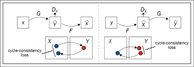
Figure 9.10: Cycle-consistency loss

To train the combined GANs, the authors added, besides the conventional GAN adversarial loss, a forward cycle-consistency loss (left figure) and a backward cycle-consistency loss (right figure). This ensures that if an image X is given as input, then after the two translations F(G(X)) ~ X the obtained image is the same, X (similarly the backward cycle-consistency loss ensures that G(F(Y)) ~ Y).

Following are some of the successful image translations by CycleGANs [7]:

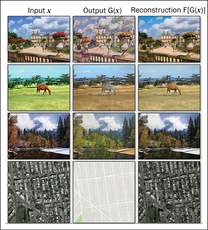
Figure 9.11: Examples of some successful CycleGAN image translations

Following are a few more examples; you can see the translation of seasons (summer winter), photo painting and vice versa, and horses zebras and vice versa [7]:

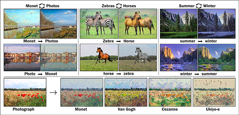
Figure 9.12: Further examples of CycleGAN translations

Later in the chapter, we will also explore a TensorFlow implementation of CycleGANs. Next, we talk about the InfoGAN, a conditional GAN where the GAN not only generates an image, but you also have a control variable to control the images generated.

InfoGAN

The GAN architectures that we have considered up to now provide us with little or no control over the generated images. The InfoGAN changes this; it provides control over various attributes of the images generated. The InfoGAN uses the concepts from information theory such that the noise term is transformed into latent code that provides predictable and systematic control over the output.

The generator in an InfoGAN takes two inputs: the latent space Z and a latent code c, thus the output of the generator is G(Z,c). The GAN is trained such that it maximizes the mutual information between the latent code c and the generated image G(Z,c). The following figure shows the architecture of the InfoGAN:

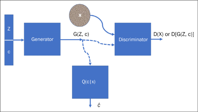
Figure 9.13: The architecture of the InfoGAN, visualized

The concatenated vector (Z,c) is fed to the generator. Q(c|X) is also a neural network. Combined with the generator, it works to form a mapping between random noise Z and its latent code c_hat. It aims to estimate c given X. This is achieved by adding a regularization term to the objective function of the conventional GAN:

The term V_G(D,G) is the loss function of the conventional GAN, and the second term is the regularization term, where is a constant. Its value was set to 1 in the paper, and I(c;G(Z,c)) is the mutual information between the latent code c and the generator-generated image G(Z,c).

Following are the exciting results of the InfoGAN on the MNIST dataset:

Figure 9.14: Results of using the InfoGAN on the MNIST dataset. Here, different rows correspond to different random samples of fixed latent codes and noise

Now, that we have seen some exciting GAN architectures, let us explore some cool applications of GAN.

Cool applications of GANs

We have seen that the generator can learn how to forge data. This means that it learns how to create new synthetic data that is created by the network that appears to be authentic and human-made. Before going into the details of some GAN code, we would like to share the results of the paper [6] (code is available online at https://github.com/hanzhanggit/StackGAN) where a GAN has been used to synthesize forged images starting from a text description. The results are impressive: the first column is the real image in the test set and all the rest of the columns are the images generated from the same text description by Stage-I and Stage-II of StackGAN. More examples are available on YouTube (https://www.youtube.com/watch?v=SuRyL5vhCIM&feature=youtu.be):

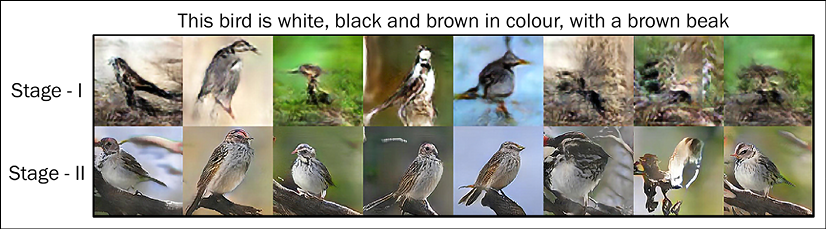
Figure 9.15: Image generation of birds, using GANs

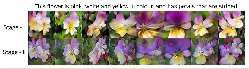
Figure 9.16: Image generation of flowers, using GANs

Now let us see how a GAN can learn to “forge” the MNIST dataset. In this case, it is a combination of GAN and CNNs used for the generator and discriminator networks. In the beginning, the generator creates nothing understandable, but after a few iterations, synthetic forged numbers are progressively clearer and clearer. In this image, the panels are ordered by increasing training epochs and you can see the quality improving among the panels:

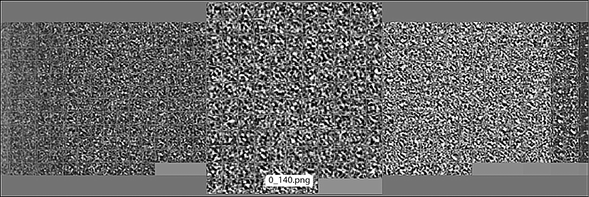
Figure 9.17: Illegible initial outputs of the GAN

As the training progresses, you can see in Figure 9.17 that the digits start taking a more recognizable form:

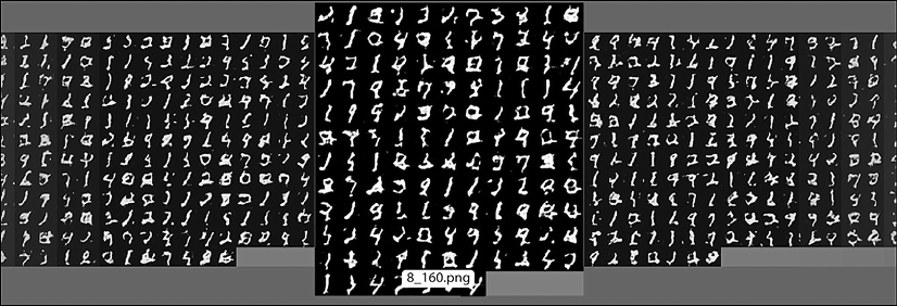
Figure 9.18: Improved outputs of the GAN, following further iterations

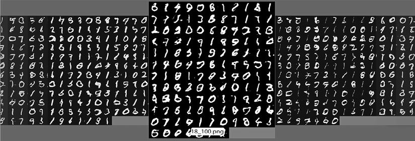
Figure 9.19: Final outputs of the GAN, showing significant improvement from previous iterations

After 10,000 epochs, you can see that the handwritten digits are even more realistic.

One of the coolest uses of GANs is doing arithmetic on faces in the generator’s vector Z. In other words, if we stay in the space of synthetic forged images, it is possible to see things like this: [smiling woman] - [neutral woman] + [neutral man] = [smiling man], or like this: [man with glasses] - [man without glasses] + [woman without glasses] = [woman with glasses]. This was shown in the paper Unsupervised Representation Learning with Deep Convolutional Generative Adversarial Networks by Alec Radford and his colleagues in 2015. All images in this work are generated by a version of GAN. They are NOT REAL. The full paper is available here: http://arxiv.org/abs/1511.06434. Following are some examples from the paper. The authors also share their code in this GitHub repo: https://github.com/Newmu/dcgan_code:

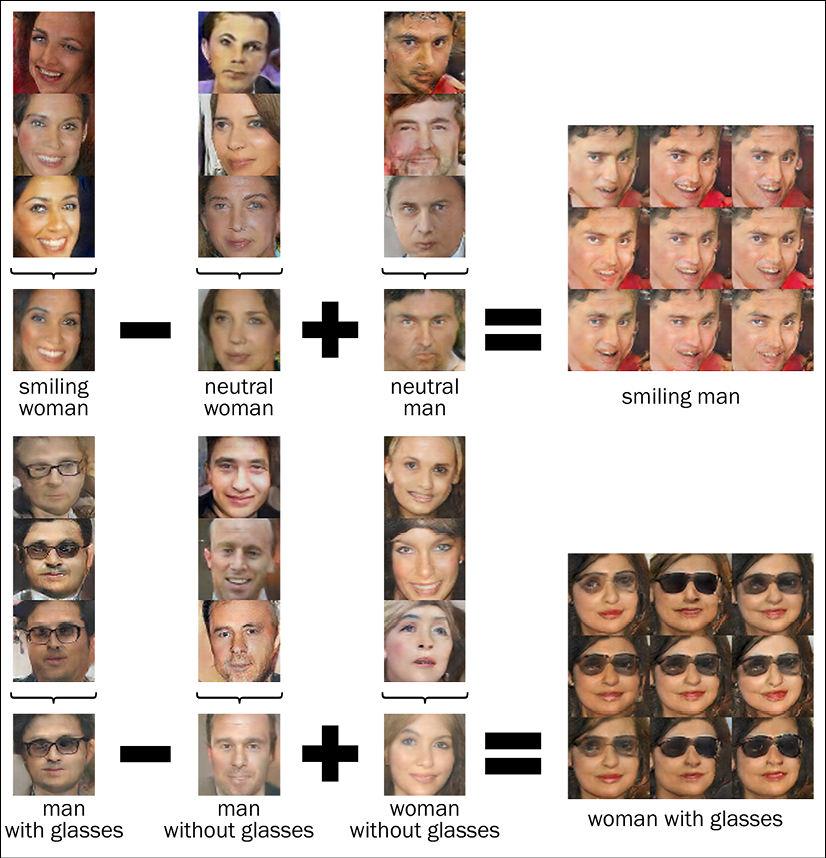
Figure 9.20: Image arithmetic using GANs

Bedrooms: Generated bedrooms after five epochs of training:

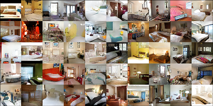
Figure 9.21: Generated bedrooms using GAN after 5 epochs of training

Album covers: These images are generated by the GAN, but look like authentic album covers:

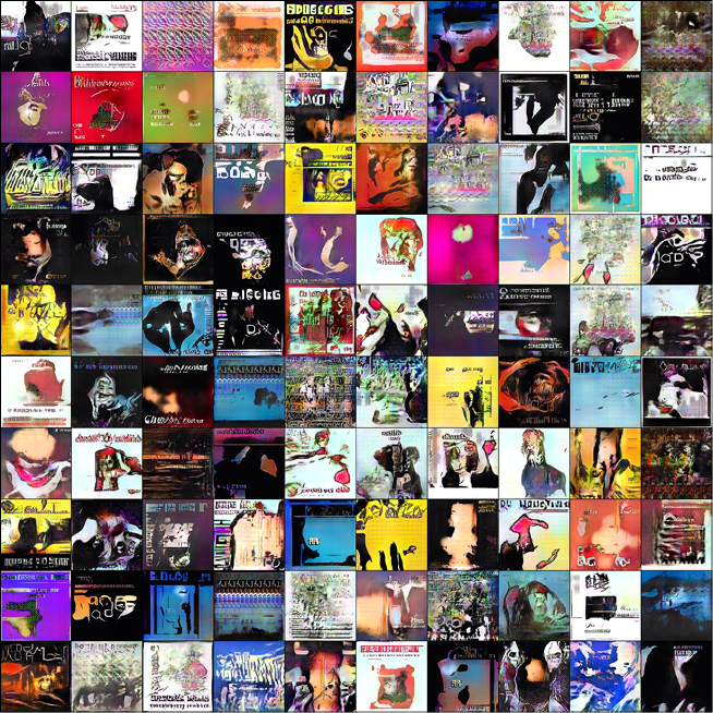
Figure 9.22: Album covers generated using DCGAN

Another cool application of GANs is the generation of artificial faces. NVIDIA introduced a model in 2018, which it named StyleGAN (the second version, StyleGAN2, was released in February 2020, and the third version in 2021), which it showed can be used to generate realistic-looking images of people. Below you can see some of the realistic-looking fake people’s faces generated by StyleGAN obtained after training of 1,000 epochs; for better results, you will need to train more:

Figure 9.23: Fake faces generated by StyleGAN

Not only does it generate fake images but like InfoGAN, you can control the features from coarse to grain. This is the official video released by NVIDIA showing how features affect the results: https://www.youtube.com/watch?v=kSLJriaOumA. They were able to do this by adding a non-linear mapping network after the Latent variable Z. The mapping network transformed the latent variable to a mapping of the same size; the output of the mapping vector is fed to different layers of the generator network, and this allows the StyleGAN to control different visual features. To know more about StyleGAN, you should read the paper A style-based generator architecture for Generative Adversarial Networks from NVIDIA Labs [10].

CycleGAN in TensorFlow

In this section, we will implement a CycleGAN in TensorFlow. The CycleGAN requires a special dataset, a paired dataset, from one domain of images to another domain. So, besides the necessary modules, we will use tensorflow_datasets as well. Also, we will make use of the library tensorflow_examples, we will directly use the generator and the discriminator from the pix2pix model defined in tensorflow_examples. The code here is adapted from the code here https://github.com/tensorflow/docs/blob/master/site/en/tutorials/generative/cyclegan.ipynb:

import tensorflow_datasets as tfds
from tensorflow_examples.models.pix2pix import pix2pix
import os
import time
import matplotlib.pyplot as plt
from IPython.display import clear_output
import tensorflow as tf

TensorFlow’s Dataset API contains a list of datasets. It has many paired datasets for CycleGANs, such as horse to zebra, apples to oranges, and so on. You can access the complete list here: https://www.tensorflow.org/datasets/catalog/cycle_gan. For our code, we will be using summer2winter_yosemite, which contains images of Yosemite (USA) in summer (Dataset A) and winter (Dataset B). We will train the CycleGAN to convert an input image of summer to winter and vice versa.

Let us load the data and get train and test images:

dataset, metadata = tfds.load('cycle_gan/summer2winter_yosemite',
                              with_info=True, as_supervised=True)
train_summer, train_winter = dataset['trainA'], dataset['trainB']
test_summer, test_winter = dataset['testA'], dataset['testB']

We need to set some hyperparameters:

BUFFER_SIZE = 1000
BATCH_SIZE = 1
IMG_WIDTH = 256
IMG_HEIGHT = 256
EPOCHS = 100
LAMBDA = 10
AUTOTUNE = tf.data.AUTOTUNE

The images need to be normalized before we train the network. For better performance, we also add random jittering to the train images; the images are first resized to size 286x286, then we randomly crop them back to the size 256x256, and finally apply the random jitter:

def normalize(input_image, label):
    input_image = tf.cast(input_image, tf.float32)
    input_image = (input_image / 127.5) - 1
    return input_image
def random_crop(image):
    cropped_image = tf.image.random_crop(image, size=[IMG_HEIGHT,
    IMG_WIDTH, 3])
    return cropped_image
def random_jitter(image):
    # resizing to 286 x 286 x 3
    image = tf.image.resize(image, [286, 286],
    method=tf.image.ResizeMethod.NEAREST_NEIGHBOR)
    # randomly cropping to 256 x 256 x 3
    image = random_crop(image)
    # random mirroring
    image = tf.image.random_flip_left_right(image)
    return image

The augmentation (random crop and jitter) is done only to the train images; therefore, we will need to separate functions for preprocessing the images, one for train data, and the other for test data:

def preprocess_image_train(image, label):
    image = random_jitter(image)
    image = normalize(image)
    return image
def preprocess_image_test(image, label):
    image = normalize(image)
    return image

The preceding functions, when applied to images, will normalize them in the range [-1,1] and apply augmentation to train images. Let us apply this to our train and test datasets and create a data generator that will provide images for training in batches:

train_summer = train_summer.cache().map(
    preprocess_image_train, num_parallel_calls=AUTOTUNE).shuffle(
    BUFFER_SIZE).batch(BATCH_SIZE)
train_winter = train_winter.cache().map(
    preprocess_image_train, num_parallel_calls=AUTOTUNE).shuffle(
    BUFFER_SIZE).batch(BATCH_SIZE)
test_summer = test_summer.map(
    preprocess_image_test,
    num_parallel_calls=AUTOTUNE).cache().shuffle(
    BUFFER_SIZE).batch(BATCH_SIZE)
test_winter = test_winter.map(
    preprocess_image_test,
    num_parallel_calls=AUTOTUNE).cache().shuffle(
    BUFFER_SIZE).batch(BATCH_SIZE)

In the preceding code, the argument num_parallel_calls allows one to take benefit from multiple CPU cores in the system; one should set its value to the number of CPU cores in your system. If you are not sure, use the AUTOTUNE = tf.data.AUTOTUNE value so that TensorFlow dynamically determines the right number for you.

As mentioned in the beginning, we use a generator and discriminator from the pix2pix model defined in the tensorflow_examples module. We will have two generators and two discriminators:

OUTPUT_CHANNELS = 3
generator_g = pix2pix.unet_generator(OUTPUT_CHANNELS, norm_type='instancenorm')
generator_f = pix2pix.unet_generator(OUTPUT_CHANNELS, norm_type='instancenorm')
discriminator_x = pix2pix.discriminator(norm_type='instancenorm', target=False)
discriminator_y = pix2pix.discriminator(norm_type='instancenorm', target=False)

Before moving ahead with the model definition, let us see the images. Each image is processed before plotting so that its intensity is normal:

to_winter = generator_g(sample_summer)
to_summer = generator_f(sample_winter)
plt.figure(figsize=(8, 8))
contrast = 8
imgs = [sample_summer, to_winter, sample_winter, to_summer]
title = ['Summer', 'To Winter', 'Winter', 'To Summer']
for i in range(len(imgs)):
  plt.subplot(2, 2, i+1)
  plt.title(title[i])
  if i % 2 == 0:
    plt.imshow(imgs[i][0] * 0.5 + 0.5)
  else:
    plt.imshow(imgs[i][0] * 0.5 * contrast + 0.5)
plt.show()

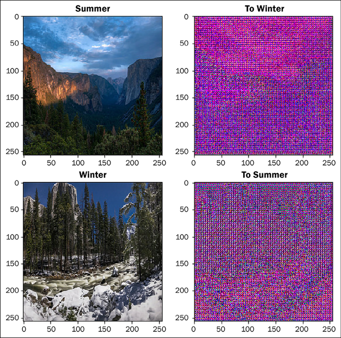
Figure 9.24: The input of GAN 1 and output of GAN 2 in CycleGAN architecture before training

We next define the loss and optimizers. We retain the same loss functions for generator and discriminator as we did in DCGAN:

loss_obj = tf.keras.losses.BinaryCrossentropy(from_logits=True)
def discriminator_loss(real, generated):
    real_loss = loss_obj(tf.ones_like(real), real)
    generated_loss = loss_obj(tf.zeros_like(generated), generated)
    total_disc_loss = real_loss + generated_loss
    return total_disc_loss * 0.5
def generator_loss(generated):
    return loss_obj(tf.ones_like(generated), generated)

Since there are now four models, two generators and two discriminators, we need to define four optimizers:

generator_g_optimizer = tf.keras.optimizers.Adam(2e-4, beta_1=0.5)
generator_f_optimizer = tf.keras.optimizers.Adam(2e-4, beta_1=0.5)
discriminator_x_optimizer = tf.keras.optimizers.Adam(2e-4, beta_1=0.5)
discriminator_y_optimizer = tf.keras.optimizers.Adam(2e-4, beta_1=0.5)

Additionally, in the CycleGAN, we require to define two more loss functions, first the cycle-consistency loss; we can use the same function for forward and backward cycle-consistency loss calculation. The cycle-consistency loss ensures that the result is close to the original input:

def calc_cycle_loss(real_image, cycled_image):
    loss1 = tf.reduce_mean(tf.abs(real_image - cycled_image))
    return LAMBDA * loss1

We also need to define an identity loss, which ensures that if an image Y is fed to the generator, it would yield the real image Y or an image similar to Y. Thus, if we give our summer image generator an image of summer as input, it should not change it much:

def identity_loss(real_image, same_image):
    loss = tf.reduce_mean(tf.abs(real_image - same_image))
    return LAMBDA * 0.5 * loss

Now we define the function that trains the generator and discriminator in a batch, a pair of images at a time. The two discriminators and the two generators are trained via this function with the help of the tape gradient. The training step can be divided into four parts:

1. Get the output images from the two generators.
2. Calculate the losses.
3. Calculate the gradients.
4. And finally, apply the gradients:

   @tf.function
   def train_step(real_x, real_y):
       # persistent is set to True because the tape is used
       # more than once to calculate the gradients.
     with tf.GradientTape(persistent=True) as tape:
       # Generator G translates X -> Y
       # Generator F translates Y -> X.
       
       fake_y = generator_g(real_x, training=True)
       cycled_x = generator_f(fake_y, training=True)
       fake_x = generator_f(real_y, training=True)
       cycled_y = generator_g(fake_x, training=True)
       # same_x and same_y are used for identity loss.
       same_x = generator_f(real_x, training=True)
       same_y = generator_g(real_y, training=True)
       disc_real_x = discriminator_x(real_x, training=True)
       disc_real_y = discriminator_y(real_y, training=True)
       disc_fake_x = discriminator_x(fake_x, training=True)
       disc_fake_y = discriminator_y(fake_y, training=True)
       # calculate the loss
       gen_g_loss = generator_loss(disc_fake_y)
       gen_f_loss = generator_loss(disc_fake_x)
       
       total_cycle_loss = calc_cycle_loss(real_x, cycled_x) + 
       calc_cycle_loss(real_y, cycled_y)
       
       # Total generator loss = adversarial loss + cycle loss
       total_gen_g_loss = gen_g_loss + total_cycle_loss + 
       identity_loss(real_y, same_y)
       total_gen_f_loss = gen_f_loss + total_cycle_loss + 
       identity_loss(real_x, same_x)
       disc_x_loss = discriminator_loss(disc_real_x,
       disc_fake_x)
       disc_y_loss = discriminator_loss(disc_real_y,
       disc_fake_y)
       # Calculate the gradients for generator and discriminator
       generator_g_gradients = tape.gradient(total_gen_g_loss,
       generator_g.trainable_variables)
       generator_f_gradients = tape.gradient(total_gen_f_loss,
       generator_f.trainable_variables)
       discriminator_x_gradients = tape.gradient(disc_x_loss,
       discriminator_x.trainable_variables)
       discriminator_y_gradients = tape.gradient(disc_y_loss,
       discriminator_y.trainable_variables)
       # Apply the gradients to the optimizer
       generator_g_optimizer.apply_gradients(zip(generator_g_gradients, generator_g.trainable_variables))
       generator_f_optimizer.apply_gradients(zip(generator_f_gradients, generator_f.trainable_variables))
       discriminator_x_optimizer.apply_gradients(zip(discriminator_x_gradients, discriminator_x.trainable_variables))
       discriminator_y_optimizer.apply_gradients(zip(discriminator_y_gradients, discriminator_y.trainable_variables))
   

We define checkpoints to save the model weights. Since it can take a while to train a sufficiently good CycleGAN, we save the checkpoints, and if we start next, we can start with loading the existing checkpoints – this will ensure that model starts learning from where it left:

checkpoint_path = "./checkpoints/train"
ckpt = tf.train.Checkpoint(generator_g=generator_g,
                           generator_f=generator_f,
                           discriminator_x=discriminator_x,
                           discriminator_y=discriminator_y,
                           generator_g_optimizer=generator_g_optimizer,
generator_f_optimizer=generator_f_optimizer,
discriminator_x_optimizer=discriminator_x_optimizer,
discriminator_y_optimizer=discriminator_y_optimizer)
ckpt_manager = tf.train.CheckpointManager(ckpt, checkpoint_path, max_to_keep=5)
# if a checkpoint exists, restore the latest checkpoint.
if ckpt_manager.latest_checkpoint:
    ckpt.restore(ckpt_manager.latest_checkpoint)
    print ('Latest checkpoint restored!!')

Let us now combine it all and train the network for 100 epochs. Please remember that in the paper, the test network was trained for 200 epochs, so our results will not be that good:

for epoch in range(EPOCHS):
    start = time.time()
    n = 0
    for image_x, image_y in tf.data.Dataset.zip((train_summer, train_winter)):
        train_step(image_x, image_y)
        if n % 10 == 0:
            print ('.', end='')
        n += 1
    clear_output(wait=True)
    # Using a consistent image (sample_summer) so that the progress of
    # the model is clearly visible.
    generate_images(generator_g, sample_summer)
    if (epoch + 1) % 5 == 0:
        ckpt_save_path = ckpt_manager.save()
        print ('Saving checkpoint for epoch {} at {}'.format(epoch+1,
                                                             ckpt_save_path))
    print ('Time taken for epoch {} is {} sec
'.format(epoch + 1,
                                                        time.time()-start))

You can see some of the images generated by our CycleGAN. Generator A takes in summer photos and converts them to winter, while generator B takes in winter photos and converts them to summer:

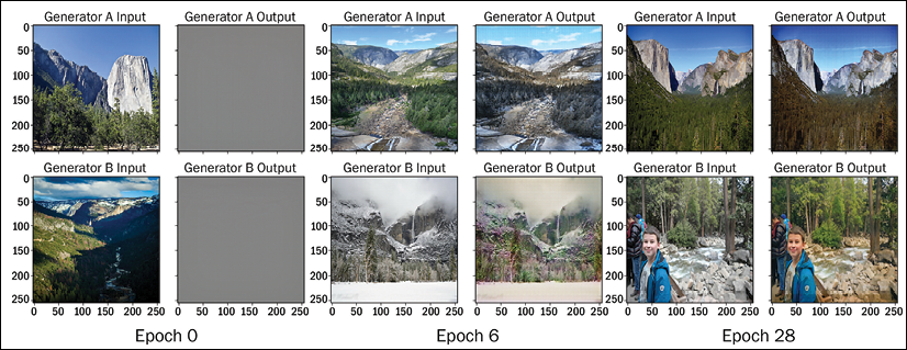
Figure 9.25: Images using CycleGAN after training

We suggest you experiment with other datasets in the TensorFlow CycleGAN datasets. Some will be easy like apples and oranges, but some will require much more training. The authors also maintain a GitHub repository where they have shared their own implementation in PyTorch along with the links to implementations in other frameworks including TensorFlow: https://github.com/junyanz/CycleGAN.

Flow-based models for data generation

While both VAEs (Chapter 8, Autoencoders) and GANs do a good job of data generation, they do not explicitly learn the probability density function of the input data. GANs learn by converting the unsupervised problem to a supervised learning problem.

VAEs try to learn by optimizing the maximum log-likelihood of the data by maximizing the Evidence Lower Bound (ELBO). Flow-based models differ from the two in that they explicitly learn data distribution . This offers an advantage over VAEs and GANs, because this makes it possible to use flow-based models for tasks like filling incomplete data, sampling data, and even identifying bias in data distributions. Flow-based models accomplish this by maximizing the log-likelihood estimation. To understand how, let us delve a little into its math.

Let be the probability density of data D, and let be the probability density approximated by our model M. The goal of a flow-based model is to find the model parameters such that the distance between two is minimum, i.e.:

If we use the KL divergence as our distance metrics, the expression above reduces to:

This equation represents minimizing the Negative Log-Likelihood (NLL) (equivalent to maximizing log-likelihood estimation.)

The basic architecture of flow-based models consists of a series of invertible functions, as shown in the figure below. The challenge is to find the function f(x), such that its inverse f^-1(x) generates x’, the reconstructed version of the input x:

Figure 9.26: Architecture of flow-based model

There are mainly two ways flow-based models are implemented:

• Normalized Flow: Here, the basic idea is to use a series of simple invertible functions to transform the complex input. As we flow through the sequence of transformations, we repeatedly substitute the variable with a new one, as per the change of variables theorem (https://archive.lib.msu.edu/crcmath/math/math/c/c210.htm), and finally, we obtain a probability distribution of the target variable. The path that the variables z_i traverse is the flow and the complete chain formed by the successive distributions is called the normalizing flow.

  The RealNVP (Real-valued Non-Volume Preserving) model proposed by Dinh et al., 2017, NICE (Non-linear Independent Components Estimation) by Dinh et al., 2015, and Glow by Knigma and Dhariwal, 2018, use the normalized flow trick:

  

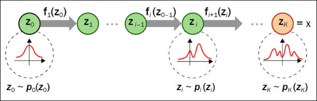
  Figure 9.27: Normalizing flow model: https://lilianweng.github.io/posts/2018-10-13-flow-models/

• Autoregressive Flow: Models like MADE (Masked Autoencoder for Distribution Estimation), PixelRNN, and wavenet are based on autoregressive models. Here, each dimension in a vector variable is dependent on the previous dimensions. Thus, the probability of observing depends only on , and therefore, the product of these conditional probabilities gives us the probability of the entire sequence.

Lilian Weng’s blog (https://lilianweng.github.io/posts/2018-10-13-flow-models/) provides a very good description of flow-based models.

Diffusion models for data generation

The 2021 paper Diffusion Models Beat GANs on Image synthesis by two OpenAI research scientists Prafulla Dhariwal and Alex Nichol garnered a lot of interest in diffusion models for data generation.

Using the Frechet Inception Distance (FID) as the metrics for evaluation of generated images, they were able to achieve an FID score of 3.85 on a diffusion model trained on ImageNet data:

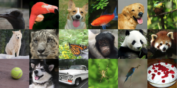
Figure 9.28: Selected samples of images generated from ImageNet (FID 3.85). Image Source: Dhariwal, Prafulla, and Alexander Nichol. “Diffusion models beat GANs on image synthesis.” Advances in Neural Information Processing Systems 34 (2021)

The idea behind diffusion models is very simple. We take our input image , and at each time step (forward step), we add a Gaussian noise to it (diffusion of noise) such that after time steps, the original image is no longer decipherable. And then find a model that can, starting from a noisy input, perform the reverse diffusion and generate a clear image:

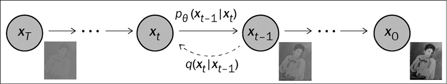
Figure 9.29: Graphical model as a Markov chain for the forward and reverse diffusion process

The only problem is that while the conditional probabilities can be obtained using the reparameterization trick, the reverse conditional probability is unknown. We train a neural network model to approximate these conditional probabilities. Below is the training and the sampling algorithm used by Ho et al., 2020, in their Denoising Diffusion Probabilistic Models paper:

Table 9.1: Training and sampling steps used by Ho et al., 2020

Diffusion models offer both tractability and flexibility – two conflicting objectives in generative models. However, they rely on a long Markov chain of diffusion steps and thus are computationally expensive. There is a lot of traction in diffusion models, and we hope that in the near future there will be algorithms that can give as fast sampling as GANs.

Summary

This chapter explored one of the most exciting deep neural networks of our times: GANs. Unlike discriminative networks, GANs have the ability to generate images based on the probability distribution of the input space. We started with the first GAN model proposed by Ian Goodfellow and used it to generate handwritten digits. We next moved to DCGANs where convolutional neural networks were used to generate images and we saw the remarkable pictures of celebrities, bedrooms, and even album artwork generated by DCGANs. Finally, the chapter delved into some awesome GAN architectures: the SRGAN, CycleGAN, InfoGAN, and StyleGAN. The chapter also included an implementation of the CycleGAN in TensorFlow 2.0.

In this chapter and the ones before it, we have been continuing with different unsupervised learning models, with both autoencoders and GANs examples of self-supervised learning; the next chapter will further detail the difference between self-supervised, joint, and contrastive learning.

References

1. Goodfellow, Ian J. (2014). On Distinguishability Criteria for Estimating Generative Models. arXiv preprint arXiv:1412.6515: https://arxiv.org/pdf/1412.6515.pdf
2. Dumoulin, Vincent, and Visin, Francesco. (2016). A guide to convolution arithmetic for deep learning. arXiv preprint arXiv:1603.07285: https://arxiv.org/abs/1603.07285
3. Salimans, Tim, et al. (2016). Improved Techniques for Training GANs. Advances in neural information processing systems: http://papers.nips.cc/paper/6125-improved-techniques-for-training-gans.pdf
4. Johnson, Justin, Alahi, Alexandre, and Fei-Fei, Li. (2016). Perceptual Losses for Real-Time Style Transfer and Super-Resolution. European conference on computer vision. Springer, Cham: https://arxiv.org/abs/1603.08155
5. Radford, Alec, Metz, Luke., and Chintala, Soumith. (2015). Unsupervised Representation Learning with Deep Convolutional Generative Adversarial Networks. arXiv preprint arXiv:1511.06434: https://arxiv.org/abs/1511.06434
6. Ledig, Christian, et al. (2017). Photo-Realistic Single Image Super-Resolution Using a Generative Adversarial Network. Proceedings of the IEEE conference on computer vision and pattern recognition: http://openaccess.thecvf.com/content_cvpr_2017/papers/Ledig_Photo-Realistic_Single_Image_CVPR_2017_paper.pdf
7. Zhu, Jun-Yan, et al. (2017). Unpaired Image-to-Image Translation using Cycle-Consistent Adversarial Networks. Proceedings of the IEEE international conference on computer vision: http://openaccess.thecvf.com/content_ICCV_2017/papers/Zhu_Unpaired_Image-To-Image_Translation_ICCV_2017_paper.pdf
8. Karras, Tero, Laine, Samuli, and Aila, Timo. (2019). A style-based generator architecture for generative adversarial networks. In Proceedings of the IEEE/CVF conference on computer vision and pattern recognition, pp. 4401-4410.
9. Chen, Xi, et al. (2016). InfoGAN: Interpretable Representation Learning by Information Maximizing Generative Adversarial Nets. Advances in neural information processing systems: https://arxiv.org/abs/1606.03657
10. TensorFlow implementation of the StyleGAN: https://github.com/NVlabs/stylegan

Join our book’s Discord space

Join our Discord community to meet like-minded people and learn alongside more than 2000 members at: https://packt.link/keras