13

An Introduction to AutoML

The goal of AutoML is to enable domain experts who are unfamiliar with machine learning technologies to use ML techniques easily.

In this chapter, we will go through a practical exercise using Google Cloud Platform and do quite a bit of hands-on work after briefly discussing the fundamentals.

We will cover:

• Automatic data preparation
• Automatic feature engineering
• Automatic model generation
• AutoKeras
• Google Cloud AutoML with its multiple solutions for table, vision, text, translation, and video processing

Let’s begin with an introduction to AutoML.

What is AutoML?

During the previous chapters, we introduced several models used in modern machine learning and deep learning. For instance, we have seen architectures such as dense networks, CNNs, RNNs, autoencoders, and GANs.

Two observations are in order. First, these architectures are manually designed by deep learning experts and are not necessarily easy to explain to non-experts. Second, the composition of these architectures themselves was a manual process, which involved a lot of human intuition and trial and error.

Today, one primary goal of artificial intelligence research is to achieve Artificial General Intelligence (AGI) – the intelligence of a machine that can understand and automatically learn any type of work or activity that a human being can do. It should be noted that many researchers do not believe that AGI is achievable because there is not only one form of intelligence but many forms.

Personally, I tend to agree with this view. See https://twitter.com/ylecun/status/1526672565233758213 for Yann LeCun’s position on this subject. However, the reality was very different before AutoML research and industrial applications started. Indeed, before AutoML, designing deep learning architectures was very similar to crafting – the activity or hobby of making decorative articles by hand.

Take, for instance, the task of recognizing breast cancer from X-rays. After reading the previous chapters, you will probably think that a deep learning pipeline created by composing several CNNs may be an appropriate tool for this purpose. That is probably a good intuition to start with. The problem is that it is not easy to explain to the users of your model why a particular composition of CNN works well within the breast cancer detection domain. Ideally, you want to provide easily accessible deep learning tools to the domain experts (in this case, medical professionals) without such a tool requiring a strong machine learning background.

The other problem is that it is not easy to understand whether or not there are variants (for example, different compositions) of the original manually crafted model that can achieve better results. Ideally, you want to provide deep learning tools for exploring the space of variants (for example, different compositions) in a more principled and automatic way.

So, the central idea of AutoML is to reduce the steep learning curve and the huge costs of handcrafting machine learning solutions by making the whole end-to-end machine learning pipeline more automated. To this end, we assume that the AutoML pipeline consists of three macro-steps: data preparation, feature engineering, and automatic model generation, as shown in Figure 13.1:

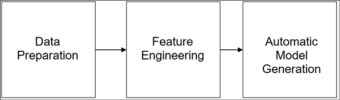
Figure 13.1: Three steps of an AutoML pipeline

Throughout the initial part of this chapter, we are going to discuss these three steps in detail. Then, we will focus on Google Cloud AutoML.

Achieving AutoML

How can AutoML achieve the goal of end-to-end automatization? Well, you have probably already guessed that a natural choice is to use machine learning – that’s very cool. AutoML uses ML for automating ML pipelines.

What are the benefits? Automating the creation and tuning of machine learning end to end offers simpler solutions, reduces the time to produce them, and ultimately might produce architectures that could potentially outperform models that were crafted by hand.

Is this a closed research area? Quite the opposite. At the beginning of 2022, AutoML is a very open research field, which is not surprising, as the initial paper drawing attention to AutoML was published at the end of 2016.

Automatic data preparation

The first stage of a typical machine learning pipeline deals with data preparation (recall the pipeline in Figure 13.1). There are two main aspects that should be taken into account: data cleansing and data synthesis:

Data cleansing is about improving the quality of data by checking for wrong data types, missing values, and errors, and by applying data normalization, bucketization, scaling, and encoding. A robust AutoML pipeline should automate all of these mundane but extremely important steps as much as possible.

Data synthesis is about generating synthetic data via augmentation for training, evaluation, and validation. Normally, this step is domain-specific. For instance, we have seen how to generate synthetic CIFAR10-like images (Chapter 4) by using cropping, rotation, resizing, and flipping operations. One can also think about generating additional images or video via GANs (see Chapter 9) and using the augmented synthetic dataset for training. A different approach should be taken for text, where it is possible to train RNNs (Chapter 5) to generate synthetic text or to adopt more NLP techniques such as BERT, Seq2Seq, or Transformers (see Chapter 6) to annotate or translate text across languages and then translate it back to the original one – another domain-specific form of augmentation.

A different approach is to generate synthetic environments where machine learning can occur. This became very popular in reinforcement learning and gaming, especially with toolkits such as OpenAI Gym, which aims to provide an easy-to-set-up simulation environment with a variety of different (gaming) scenarios.

Put simply, we can say that synthetic data generation is another option that should be provided by AutoML engines. Frequently, the tools used are very domain-specific and what works for image or video would not necessarily work in other domains such as text. Therefore, we need a (quite) large set of tools for performing synthetic data generation across domains.

Automatic feature engineering

Feature engineering is the second step of a typical machine learning pipeline (see Figure 13.1). It consists of three major steps: feature selection, feature construction, and feature mapping. Let’s look at each of them in turn:

Feature selection aims at selecting a subset of meaningful features by discarding those that are making little contribution to the learning task. In this context, “meaningful” truly depends on the application and the domain of your specific problem.

Feature construction has the goal of building new derived features, starting from the basic ones. Frequently, this technique is used to allow better generalization and to have a richer representation of the data.

Feature mapping aims at altering the original feature space by means of a mapping function. This can be implemented in multiple ways; for instance, it can use autoencoders (see Chapter 8), PCA (see Chapter 7), or clustering (see Chapter 7).

In short, feature engineering is an art based on intuition, trial and error, and a lot of human experience. Modern AutoML engines aim to make the entire process more automated, requiring less human intervention.

Automatic model generation

Model generation and hyperparameter tuning is the typical third macro-step of a machine learning pipeline (see Figure 13.1).

Model generation consists of creating a suitable model for solving specific tasks. For instance, you will probably use CNNs for visual recognition, and you will use RNNs for either time series analysis or for sequences. Of course, many variants are possible, each of which is manually crafted through a process of trial and error and works for very specific domains.

Hyperparameter tuning happens once the model is manually crafted. This process is generally very computationally expensive and can significantly change the quality of the results in a positive way. That’s because tuning the hyperparameters can help to optimize our model further.

Automatic model generation is the ultimate goal of any AutoML pipeline. How can this be achieved? One approach consists of generating the model by combining a set of primitive operations including convolution, pooling, concatenation, skip connections, recurrent neural networks, autoencoders, and pretty much all the deep learning models we have encountered throughout this book. These operations constitute a (typically very large) search space to be explored, and the goal is to make this exploration as efficient as possible. In AutoML jargon, the exploration is called NAS, or Neural Architecture Search. The seminal paper on AutoML [1] was produced in November 2016. The key idea (see Figure 13.2) is to use reinforcement learning (RL, see Chapter 11). An RNN acts as the controller, and it generates the model descriptions of candidate neural networks. RL is used to maximize the expected accuracy of the generated architectures on a validation set.

On the CIFAR-10 dataset, this method, starting from scratch, designed a novel network architecture that rivals the best human-invented architecture in terms of test set accuracy. The CIFAR-10 model achieves a test error rate of 3.65, which is 0.09 percent better and 1.05x faster than the previous state-of-the-art model that used a similar architectural scheme. On the Penn Treebank dataset, the model can compose a novel recurrent cell that outperforms the widely used LSTM cell (see Chapter 9) and other state-of-the-art baselines. The cell achieves a test set perplexity of 62.4 on the Penn Treebank, which is 3.6 better than the previous state-of-the-art model.

The key outcome of the paper is shown in Figure 13.2. A controller network based on RNNs produces a sample architecture A with probability p. This candidate architecture A is trained by a child network to get a candidate accuracy R. Then a gradient of p is computed and scaled by R to update the controller. This reinforcement learning operation is computed in a cycle a number of times. The process of generating an architecture stops if the number of layers exceeds a certain value.

The details of how an RL-based policy gradient method is used by the controller RNN to generate better architectures are in [1]. Here we emphasize the fact that NAS uses a meta-modeling algorithm based on Q-learning with an ϵ-greedy exploration strategy and with experience replay (see Chapter 11) to explore the model search space:

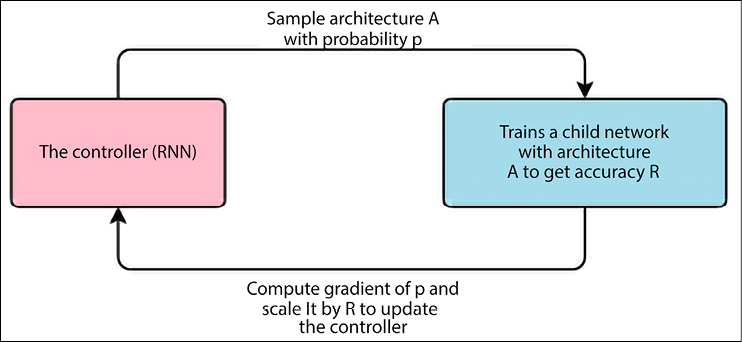
Figure 13.2: NAS with recurrent neural networks

Since the original paper in late 2016, a Cambrian explosion of model generation techniques has been observed. Initially, the goal was to generate the entire model in one single step. Later, a cell-based approach was proposed where the generation is divided into two macro-steps: first, a cell structure is automatically built, and then a predefined number of discovered cells are stacked together to generate an entire end-to-end architecture [2]. This Efficient Neural Architecture Search (ENAS) delivers strong empirical performance using significantly fewer GPU hours compared with all existing automatic model design approaches, and notably, is 1,000x less computationally expensive than standard neural architecture search (in 2018). Here, the primary ENAS goal is to reduce the search space via hierarchical composition. Variants of the cell-based approach have been proposed including pure hierarchical methods where higher-level cells are generated by incorporating lower-level cells iteratively.

A completely different approach to NAS is to use transfer learning (see Chapter 5) to transfer the learning of an existing neural network into a new neural network in order to speed up the design [3]. In other words, we want to use transfer learning in AutoML.

Another approach is based on Genetic Programming (GP) and Evolutionary Algorithms (EAs), where the basic operations constituting the model search space are encoded into a suitable representation, and then this encoding is gradually mutated to progressively better models in a way that resembles the genetic evolution of living beings [4].

Hyperparameter tuning consists of finding the optimal combination of hyperparameters both related to learning optimization (batch size, learning rate, and so on) and model-specific ones (kernel size; number of feature maps and so on for CNNs; or number of neurons for dense or autoencoder networks, and so on). Again, the search space can be extremely large. There are three approaches generally used: Bayesian optimization, grid search, and random search.

Bayesian optimization builds a probability model of the objective function and uses it to select the most promising hyperparameters to evaluate in the true objective function.

Grid search divides the search space into a discrete grid of values and tests all the possible combinations in the grid. For instance, if there are three hyperparameters and a grid with only two candidate values for each of them, then a total of 2 x 3 = 6 combinations must be checked. There are also hierarchical variants of grid search, which progressively refine the grid for regions of the search space and provide better results. The key idea is to use a coarse grid first, and after finding a better grid region, implement a finer grid search on that region.

Random search performs a random sampling of the parameter search space, and this simple approach has been proven to work very well in many situations [5].

Now that we have briefly discussed the fundamentals, we will do quite a bit of hands-on work on Google Cloud. Let’s start.

AutoKeras

AutoKeras [6] provides functions to automatically search for architecture and hyperparameters of deep learning models. The framework uses Bayesian optimization for efficient neural architecture search. You can install the alpha version by using pip:

pip3 install autokeras # for 1.19 version

The architecture is explained in Figure 13.3 [6]:

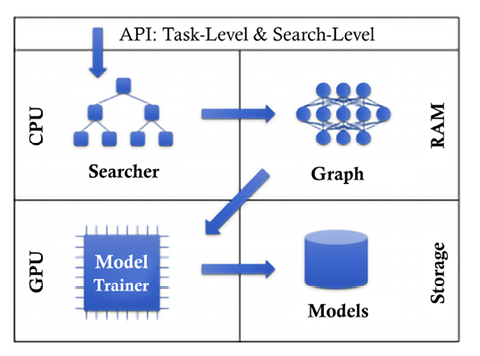
Figure 13.3: AutoKeras system overview

The architecture follows these steps:

1. The user calls the API.
2. The searcher generates neural architectures on the CPU.
3. Real neural networks with parameters are built on RAM from the neural architectures.
4. The neural network is copied to the GPU for training.
5. The trained neural networks are saved on storage devices.
6. The searcher is updated based on the training results.

Steps 2 to 6 will repeat until a time limit is reached.

Google Cloud AutoML and Vertex AI

Google Cloud AutoML (https://cloud.google.com/automl/) is a full suite of products for image, video, and text processing. AutoML can be used to train high-quality custom machine learning models with minimal effort and machine learning expertise.

Vertex AI brings together the Google Cloud services for building ML under one, unified UI and API. In Vertex AI, you can now easily train, compare, test, and deploy models. Then you can serve a model with sophisticated ways to monitor and run experiments (see https://cloud.google.com/vertex-ai).

As of 2022, the suite consists of the following components, which do not require you to know how the deep learning networks are shaped internally:

Vertex AI

• Unified platform to help you build, deploy, and scale more AI models

Structured data

• AutoML Tables: Automatically build and deploy state-of-the-art machine learning models on structured data

Sight

• AutoML Image: Derive insights from object detection and image classification, in the cloud or at the edge
• AutoML Video: Enable powerful content discovery and engaging video experiences

Language

• AutoML Text: Reveal the structure and meaning of text through machine learning
• AutoML Translation: Dynamically detect and translate between languages

In the remainder of this chapter, we will review three AutoML solutions: AutoML Tables, AutoML Text, and AutoML Video.

Using the Google Cloud AutoML Tables solution

Let’s see an example of using Google Cloud AutoML Tables. We’ll aim to import some tabular data and train a classifier on that data; we’ll use some marketing data from a bank. Note that this and the following examples might be charged by Google according to different usage criteria (please check online for the latest cost estimation – see https://cloud.google.com/products/calculator/).

The first step required is to enable the Vertex AI API:

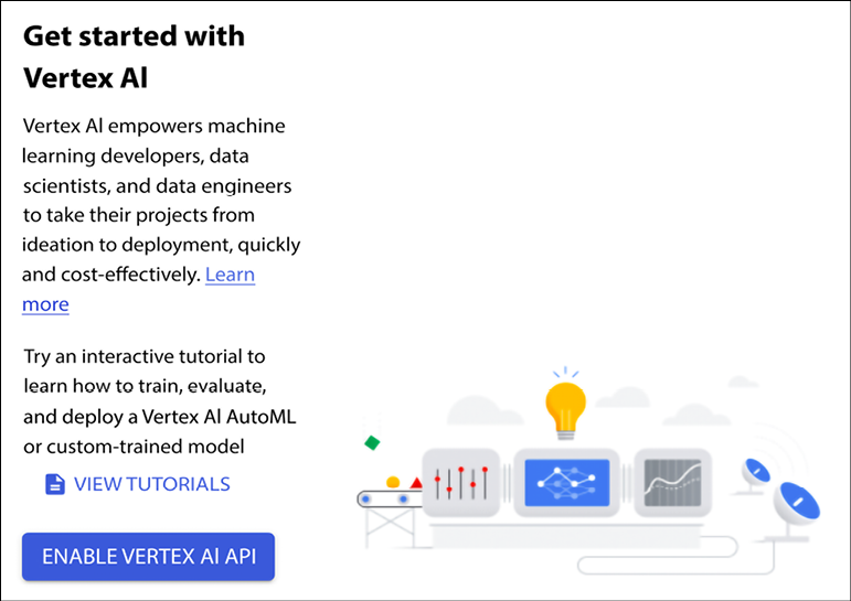
Figure 13.4: Enable the Vertex AI API

We can then select the TABULAR dataset from the console (see Figure 13.5). The name of the dataset is bank-marketing.csv:

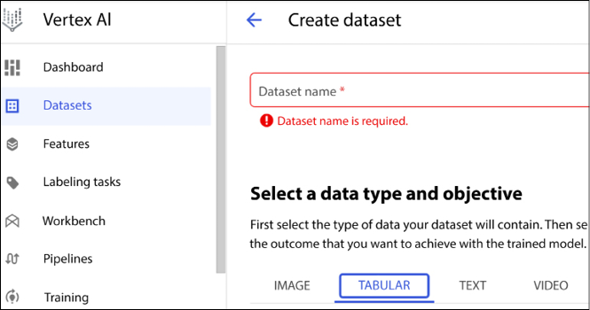
Figure 13.5: Selecting TABULAR datasets

On the next screen, we indicate that we want to load the data from CSV:

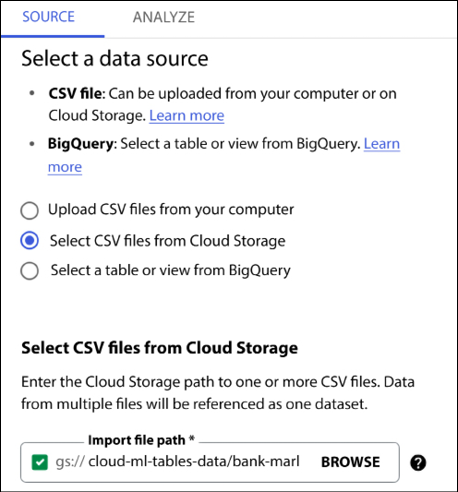
Figure 13.6: AutoML Tables – loading data from a CSV file

Next, we can train a new model, as shown in Figure 13.7:

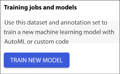
Figure 13.7: Training a new model

Several options for training are offered for Classification and Regression:

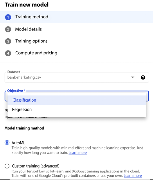
Figure 13.8: Options offered for Classification and Regression

Let’s select the target as the Deposit column. The dataset is described at https://archive.ics.uci.edu/ml/datasets/bank+marketing. The data is related to direct marketing campaigns (phone calls) of a Portuguese banking institution. The classification goal is to predict if the client will subscribe to a term deposit.

Since the selected column is categorical data, AutoML Tables will build a classification model. This will predict the target from the classes in the selected column. The classification is binary: 1 represents a negative outcome, meaning that a deposit is not made at the bank; 2 represents a positive outcome, meaning that a deposit is made at the bank, as shown in Figure 13.9:

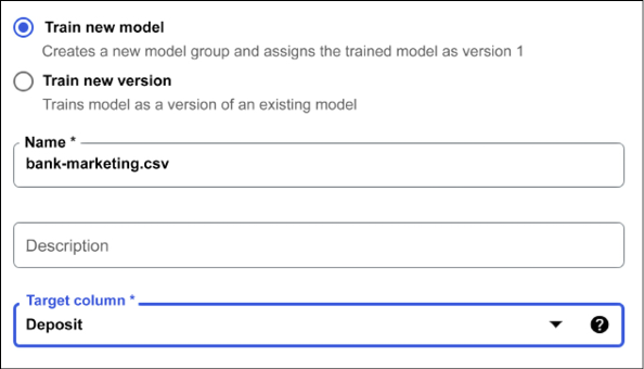
Figure 13.9: Training a new model with Target column set to Deposit

We can then inspect the dataset (see Figure 13.10), which gives us the opportunity to inspect the dataset with several features, such as names, type, missing values, distinct values, invalid values, correlation with the target, mean, and standard deviation:

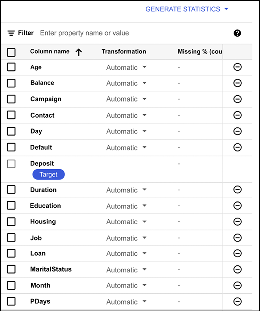
Figure 13.10: AutoML Tables – inspecting the dataset

It is now time to train the model by using the Train tab. First let’s give a budget for training, as shown in Figure 13.11:

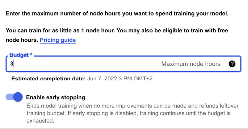
Figure 13.11: Setting up the budget for training

In this example, we accept 3 hours as our training budget. During this time, you can go and take a coffee whilst AutoML works on your behalf (see Figure 13.12). The training budget is a number between 1 and 72 for the maximum number of node hours to spend training your model. If your model stops improving before then, AutoML Tables will stop training and you’ll only be charged the money corresponding to the actual node budget used:

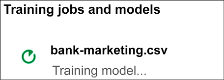
Figure 13.12: AutoML Tables training process

While training, we can check the progress, as shown in Figure 13.13:

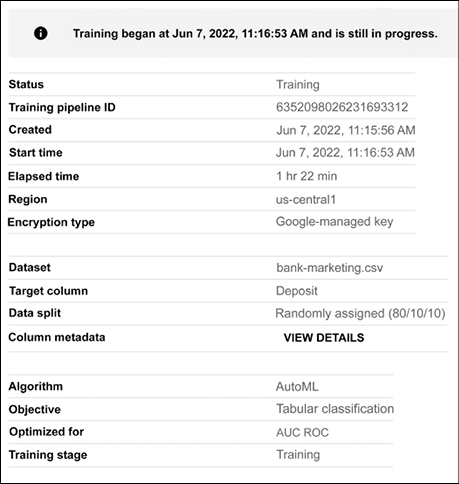
Figure 13.13: Checking the training progress

After less than one hour, Google AutoML should send an email to our inbox:

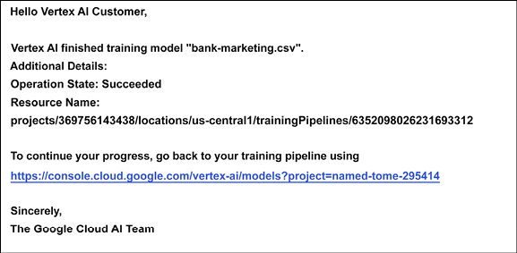
Figure 13.14: AutoML Tables: training is concluded, and an email is sent to my account

Clicking on the suggested URL, it is possible to see the results of our training. The AutoML-generated model reached an accuracy of 94% (see Figure 13.15). Remember that accuracy is the fraction of classification predictions produced by the model that were correct on a test, set which is held automatically. The log-loss (for example, the cross-entropy between the model predictions and the label values) is also provided. In the case of log-loss, a lower value indicates a higher-quality model:

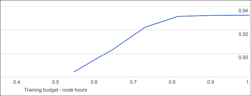
Figure 13.15: AutoML Tables – analyzing the results of our training

In addition, the Area Under the Receiver Operating Characteristic Curve (AUC ROC) is represented. This ranges from zero to one, and a higher value indicates a higher-quality model. This statistic summarizes an AUC ROC curve, which is a graph showing the performance of a classification model at all classification thresholds. The True Positive Rate (TPR) (also known as “recall”) is:

where TP is the number of true positives and FN is the number of false negatives. The False Positive Rate (FPR) is:

where FP is the number of false positives and TN is the number of true negatives.

A ROC curve plots TPR vs. FPR at different classification thresholds. In Figure 13.16 you will see the Area Under the Curve (AUC) for one threshold of a ROC curve:

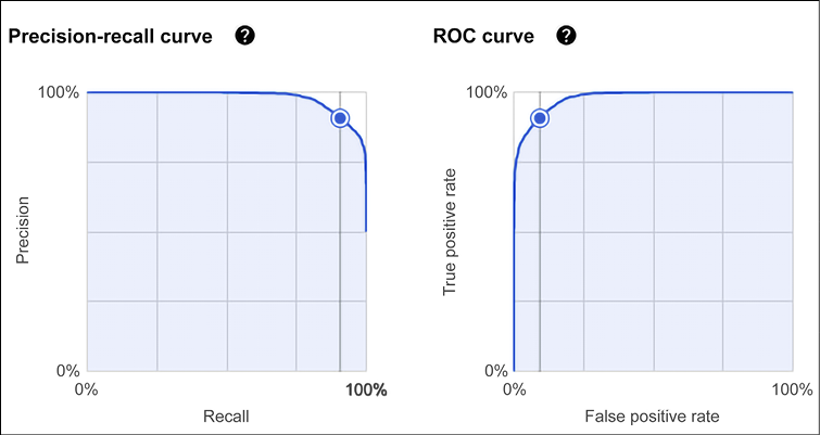
Figure 13.16: AutoML Tables – deep dive on the results of our training

It is possible to deep dive into the evaluation and access the confusion matrix (see Figure 13.17):

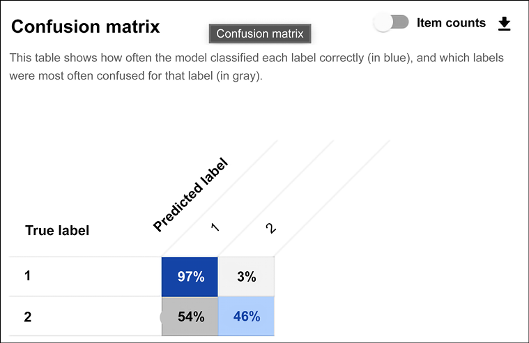
Figure 13.17: AutoML Tables – additional deep dive on the results of our training

Note that manually crafted models available in https://www.kaggle.com/uciml/adult-census-income/kernels get to an accuracy of ˜86-90%. Therefore, our model generated with AutoML is definitively a very good result!

We can also have a look at the importance of each feature in isolation, as shown in Figure 13.18:

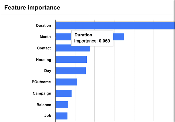
Figure 13.18: Specific importance of each feature considered in isolation

If we are happy with our results, we can then deploy the model in production via DEPLOY & TEST (see Figure 13.19). We can decide to create a Docker container deployable at the edge or we can simply use an endpoint. Let’s go for this option and just use the default setting for each available choice:

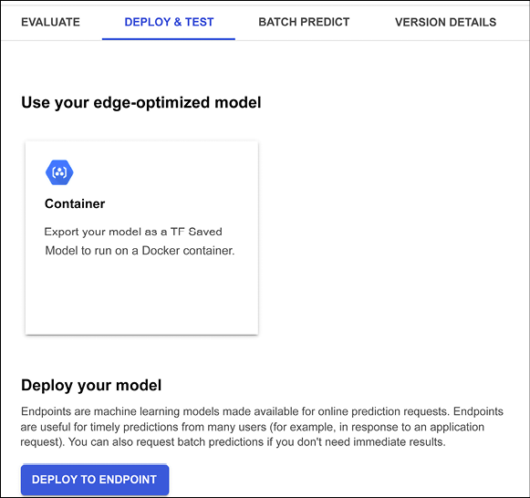
Figure 13.19: AutoML Tables – deploying in production

Then it is possible to make online predictions of income by using a REST API (see https://en.wikipedia.org/wiki/Representational_state_transfer), using this command for the example we’re looking at in this chapter, as shown in Figure 13.20:

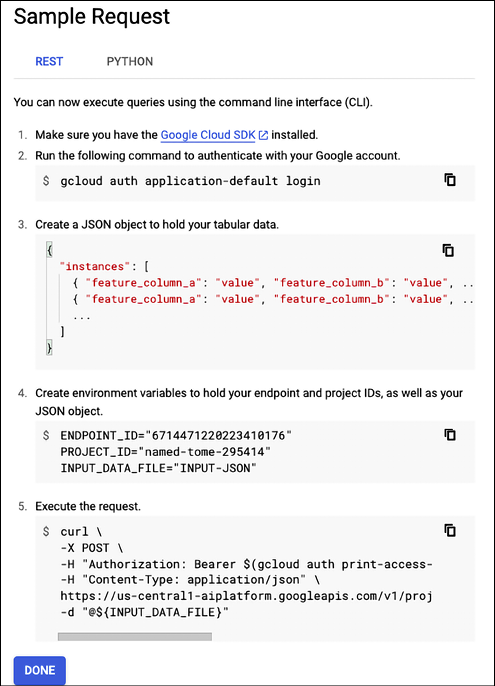
Figure 13.20: AutoML Tables – querying the deployed model in production

Put simply, we can say that Google Cloud ML is very focused on simplicity of use and efficiency for AutoML. Let’s summarize the main steps required (see Figure 13.21):

1. The dataset is imported.
2. Your dataset schema and labels are defined.
3. The input features are automatically recognized.
4. AutoML performs magic by automatically doing feature engineering, creating a model, and tuning the hyperparameters.
5. The automatically built model can then be evaluated.
6. The model is then deployed in production.

Of course, it is possible to repeat the steps 2-6 by changing the schema and the definition of the labels.

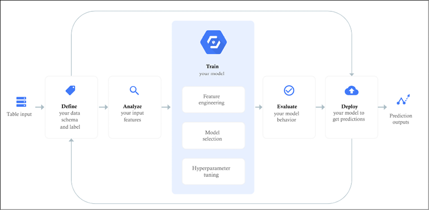
Figure 13.21: AutoML Tables – the main steps required

In this section, we have seen an example of AutoML focused on ease of use and efficiency. The progress made is shown in Faes et al. [7], quoting the paper:

”We show, to our knowledge, a first of its kind automated design and implementation of deep learning models for health-care application by non-AI experts, namely physicians. Although comparable performance to expert-tuned medical image classification algorithms was obtained in internal validations of binary and multiple classification tasks, more complex challenges, such as multilabel classification, and external validation of these models was insufficient. We believe that AI might advance medical care by improving efficiency of triage to subspecialists and the personalisation of medicine through tailored prediction models. The automated approach to prediction model design improves access to this technology, thus facilitating engagement by the medical community and providing a medium through which clinicians can enhance their understanding of the advantages and potential pitfalls of AI integration.”

In this case, Cloud AutoML Tables has been used. So, let’s look at another example.

Using the Google Cloud AutoML Text solution

In this section, we are going to build a classifier using AutoML. Let’s create a dataset for text from the Vertex AI console. We want to focus on the task of single-label classification:

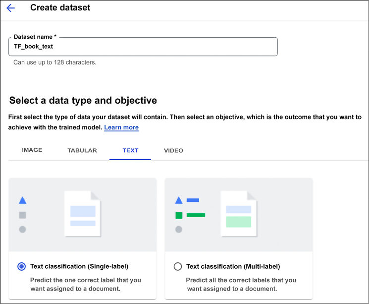
Figure 13.22: AutoML Text classification – creating a dataset

We are going to use a dataset already available online (the happy moments dataset is stored in cloud-ml-data/NL-classification/happiness.csv), load it into a dataset named happiness, and perform single-label classification (as shown in Figure 13.23). This can take several minutes or more.

We will be emailed once processing completes:

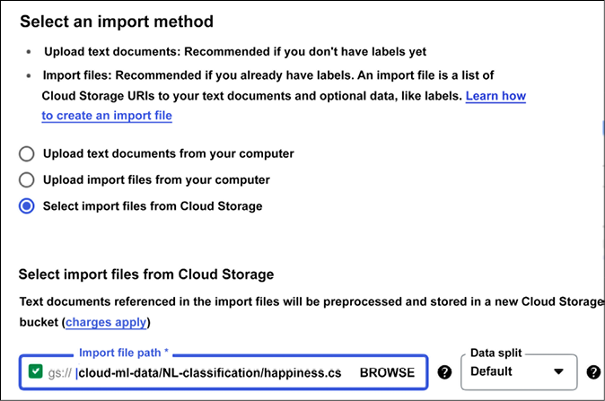
Figure 13.23: AutoML Text classification – creating the dataset

Once the dataset is loaded, you should be able to see that each text fragment is annotated with one category out of seven, as shown in Figure 13.24:

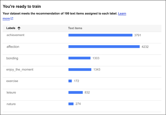
Figure 13.24: AutoML Text classification – a sample of categories

It is now time to start training the model:

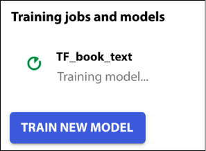
Figure 13.25: AutoML Text classification – start training

By the end, the model is built, and it achieves a good precision of 90.2% and recall of 86.7%:

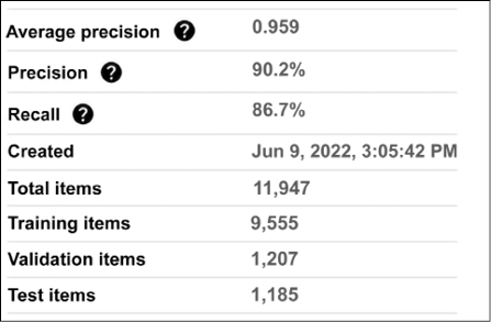
Figure 13.26: AutoML Text classification – precision and recall

We can also have a look at the precision-recall curve and precision-recall by threshold (see Figure 13.27). These curves can be used to calibrate the classifier, calibrating on the threshold (based on the prediction probabilities that are greater than the threshold):

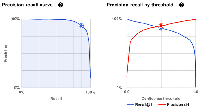
Figure 13.27: Precision-recall and Precision-recall by threshold

The confusion matrix is shown in Figure 13.28:

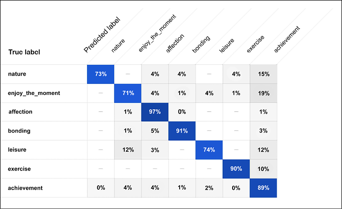
Figure 13.28: Confusion matrix for the text classification problem

Using the Google Cloud AutoML Video solution

In this solution, we are going to automatically build a new model for video classification. The intent is to be able to sort different video segments into various categories (or classes) based on their content. The first step is to create the dataset, as shown in Figure 13.29:

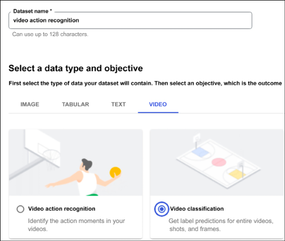
Figure 13.29: AutoML Video intelligence – a classification problem

We are going to use a collection of about 5,000 videos available in a demo already stored in a GCP bucket on automl-video-demo-data/hmdb_split1_5classes_all.csv, as shown in Figure 13.30:

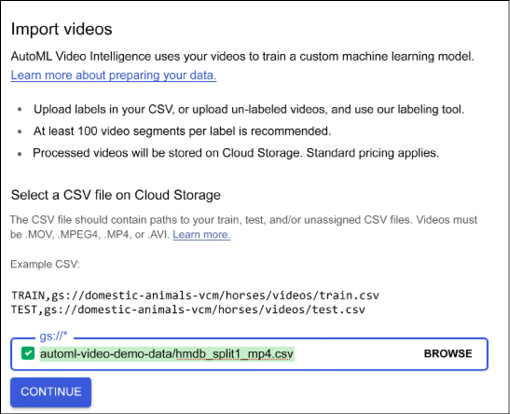
Figure 13.30. Importing the demo dataset

As usual, importing will take a while and we will be notified when it is done with an email. Once the videos are imported, we can preview them with their associated categories:

Figure 13.31: AutoML Video intelligence – imported video preview

We can now start to build a model. There are a number of options including training with AutoML, using AutoML at the edge for models to be exported at the edge, and custom models built on TensorFlow. Let’s use the default, as shown in Figure 13.32:

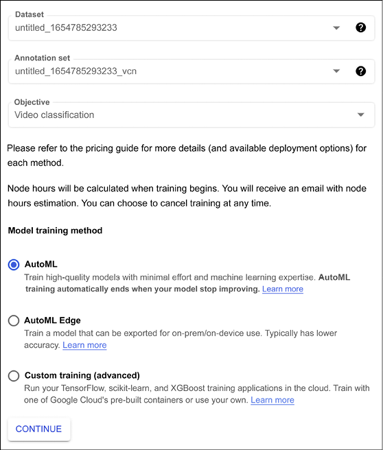
Figure 13.32: AutoML Video intelligence – warning to get more videos

In this case, we decide to run an experiment training with a few labels and divide the dataset into 20% training and 80% testing:

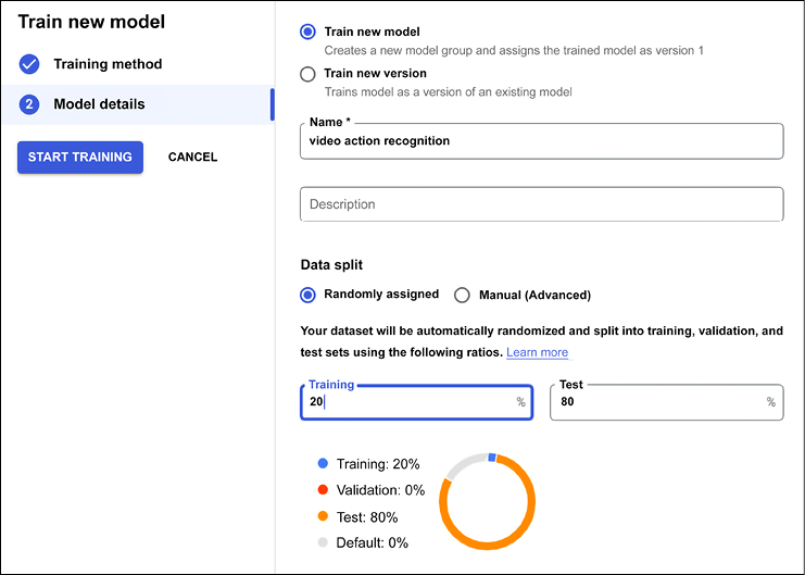
Figure 13.33: Test and Training dataset split

Once the model is trained, you can access the results from the console (Figure 13.34). In this case, we achieved a precision of 99.5% and a recall of 99.5% even though we were using only 20% of the labels for training in our experiment. We wanted to keep the training short and still achieve awesome results. You can play with the model, for instance, increasing the number of labeled videos available, to see how the performance will change:

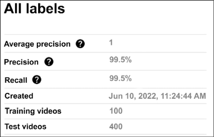
Figure 13.34: AutoML Video intelligence – evaluating the results

Let’s have a detailed look at the results. For instance, we can analyze the precision/recall graph for different levels of threshold:

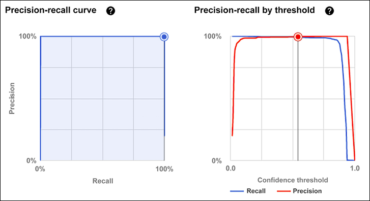
Figure 13.35: AutoML Video intelligence – precision and recall

The confusion matrix shows examples of the wrong classification of shots:

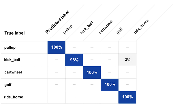
Figure 13.36: AutoML Video intelligence – confusion matrix

Cost

Training on GCP has different costs depending on the type of AutoML adopted; for example, training all the solutions presented in this chapter and serving models for testing had a cost of less than $10 in 2022. This is, however, not including the initial six hours of free discount that were available for the account (around $150 were available at the time of writing). Depending on your organizational needs, this is likely to work out significantly less than the cost of buying expensive on-premises hardware.

Summary

The goal of AutoML is to enable domain experts who are not familiar with machine learning technologies to use ML techniques easily. The primary goal is to reduce the steep learning curve and the huge costs of handcrafting machine learning solutions by making the whole end-to-end machine learning pipeline (data preparation, feature engineering, and automatic model generation) more automated.

After reviewing the state-of-the-art solution available at the end of 2022, we discussed how to use Google Cloud AutoML both for text, videos, and images, achieving results comparable to the ones achieved with handcrafted models. AutoML is probably the fastest-growing research topic and interested readers can find the latest results at https://www.automl.org/.

The next chapter discusses the math behind deep learning, a rather advanced topic that is recommended if you are interested in understanding what is going on “under the hood” when you play with neural networks.

References

1. Zoph, B., Le, Q. V. (2016). Neural Architecture Search with Reinforcement Learning. http://arxiv.org/abs/1611.01578
2. Pham, H., Guan, M. Y., Zoph, B., Le, Q. V., Dean, J. (2018). Efficient Neural Architecture Search via Parameter Sharing. https://arxiv.org/abs/1802.03268
3. Borsos, Z., Khorlin, A., Gesmundo, A. (2019). Transfer NAS: Knowledge Transfer between Search Spaces with Transformer Agents. https://arxiv.org/abs/1906.08102
4. Lu, Z., Whalen, I., Boddeti V., Dhebar, Y., Deb, K., Goodman, E., and Banzhaf, W. (2018). NSGA-Net: Neural Architecture Search using Multi-Objective Genetic Algorithm. https://arxiv.org/abs/1810.03522
5. Bergstra, J., Bengio, Y. (2012). Random search for hyper-parameter optimization. http://www.jmlr.org/papers/v13/bergstra12a.html
6. Jin, H., Song, Q., and Hu, X. (2019). Auto-Keras: An Efficient Neural Architecture Search System. https://arxiv.org/abs/1806.10282
7. Faes, L., et al. (2019). Automated deep learning design for medical image classification by health-care professionals with no coding experience: a feasibility study. The Lancet Digital Health Volume 1, Issue 5, September 2019. Pages e232-e242. https://www.sciencedirect.com/science/article/pii/S2589750019301086

Join our book’s Discord space

Join our Discord community to meet like-minded people and learn alongside more than 2000 members at: https://packt.link/keras