14

The Math Behind Deep Learning

In this chapter, we discuss the math behind deep learning. This topic is quite advanced and not necessarily required for practitioners. However, it is recommended reading if you are interested in understanding what is going on under the hood when you play with neural networks.

Here is what you will learn:

• A historical introduction
• The concepts of derivatives and gradients
• Gradient descent and backpropagation algorithms commonly used to optimize deep learning networks

Let’s begin!

History

The basics of continuous backpropagation were proposed by Henry J. Kelley [1] in 1960 using dynamic programming. Stuart Dreyfus proposed using the chain rule in 1962 [2]. Paul Werbos was the first to use backpropagation (backprop for short) for neural nets in his 1974 PhD thesis [3]. However, it wasn’t until 1986 that backpropagation gained success with the work of David E. Rumelhart, Geoffrey E. Hinton, and Ronald J. Williams published in Nature [4]. In 1987, Yann LeCun described the modern version of backprop currently used for training neural networks [5].

The basic intuition of Stochastic Gradient Descent (SGD) was introduced by Robbins and Monro in 1951 in a context different from neural networks [6]. In 2012 – or 52 years after the first time backprop was first introduced – AlexNet [7] achieved a top-5 error of 15.3% in the ImageNet 2012 Challenge using GPUs. According to The Economist [8], Suddenly people started to pay attention, not just within the AI community but across the technology industry as a whole. Innovation in this field was not something that happened overnight. Instead, it was a long walk lasting more than 50 years!

Some mathematical tools

Before introducing backpropagation, we need to review some mathematical tools from calculus. Don’t worry too much; we’ll briefly review a few areas, all of which are commonly covered in high school-level mathematics.

Vectors

We will review two basic concepts of geometry and algebra that are quite useful for machine learning: vectors and the cosine of angles. We start by giving an explanation of vectors. Fundamentally, a vector is a list of numbers. Given a vector, we can interpret it as a direction in space. Mathematicians most often write vectors as either a column x or row vector x^T. Given two column vectors u and v, we can form their dot product by computing . It can be easily proven that where is the angle between the two vectors.

Here are two easy questions for you. What is the result when the two vectors are very close? And what is the result when the two vectors are the same?

Derivatives and gradients everywhere

Derivatives are a powerful mathematical tool. We are going to use derivatives and gradients to optimize our network. Let’s look at the definition. The derivative of a function y = f(x) of a variable x is a measure of the rate at which the value y of the function changes with respect to the change of the variable x.

If x and y are real numbers, and if the graph of f is plotted against x, the derivative is the “slope” of this graph at each point.

If the function is linear , the slope is . This is a simple result of calculus, which can be derived by considering that:

In Figure 14.1, we show the geometrical meaning of , , and the angle between the linear function and the x-cartesian axis:

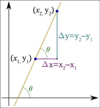
Figure 14.1: An example of a linear function and rate of change

If the function is not linear, then computing the rate of change as the mathematical limit value of the ratio of the differences as becomes infinitely small. Geometrically, this is the tangent line at as shown in Figure 14.2:

Figure 14.2: Rate of change for and the tangential line as

For instance, considering and the derivative in a given point, say x = 2, we can see that the derivative is positive , as shown in Figure 14.3:

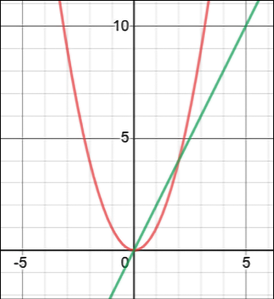
Figure 14.3: and

A gradient is a generalization of the derivative for multiple variables. Note that the derivative of a function of a single variable is a scalar-valued function, whereas the gradient of a function of several variables is a vector-valued function. The gradient is denoted with an upside-down delta , and called “del” or nabla from the Greek alphabet. This makes sense as delta indicates the change in one variable, and the gradient is the change in all variables. Suppose (e.g. the space of real numbers with m dimensions) and f maps from to ; the gradient is defined as follows:

In math, a partial derivative of a function of several variables is its derivative with respect to one of those variables, with the others held constant.

Note that it is possible to show that the gradient is a vector (a direction to move) that:

• Points in the direction of the greatest increase of a function.
• Is 0 at a local maximum or local minimum. This is because if it is 0, it cannot increase or decrease further.

The proof is left as an exercise to the interested reader. (Hint: consider Figure 14.2 and Figure 14.3.)

Gradient descent

If the gradient points in the direction of the greatest increase for a function, then it is possible to move toward a local minimum for the function by simply moving in a direction opposite to the gradient. That’s the key observation used for gradient descent algorithms, which will be used shortly.

An example is provided in Figure 14.4:

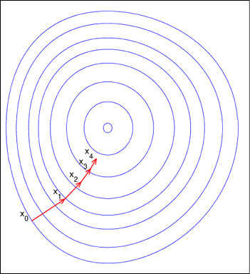
Fig.14.4: Gradient descent for a function in 3 variables

Chain rule

The chain rule says that if we have a function y = g(x) and , then the derivative is defined as follows:

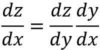
This chaining can be generalized beyond the scalar case. Suppose and with g, which maps from to , and f, which maps from to . With y = g(x) and z = f(y), we can deduce:

The generalized chain rule using partial derivatives will be used as a basic tool for the backpropagation algorithm when dealing with functions in multiple variables. Stop for a second and make sure that you fully understand it.

A few differentiation rules

It might be useful to remind ourselves of a few additional differentiation rules that will be used later:

• Constant differentiation: c’ = 0, where c is a constant.
• Variable differentiation: , when deriving the differentiation of a variable.
• Linear differentiation:
• Reciprocal differentiation:
• Exponential differentiation:

Matrix operations

There are many books about matrix calculus. Here we focus only on only a few basic operations used for neural networks. Recall that a matrix can be used to represent the weights w_ij, with , associated with the arcs between two adjacent layers. Note that by adjusting the weights we can control the “behavior” of the network and that a small change in a specific w_ij will be propagated through the network following its topology (see Figure 14.5, where the edges in bold are the ones impacted by the small change in a specific w_ij):

Figure 14.5: Propagating w_ij changes through the network via the edges in bold

Now that we have reviewed some basic concepts of calculus, let’s start applying them to deep learning. The first question is how to optimize activation functions. Well, I am pretty sure that you are thinking about computing the derivative, so let’s do it!

Activation functions

In Chapter 1, Neural Network Foundations with TF, we saw a few activation functions including sigmoid, tanh, and ReLU. In the section below, we compute the derivative of these activation functions.

Derivative of the sigmoid

Remember that the sigmoid is defined as (see Figure 14.6):

Figure 14.6: Sigmoid activation function

The derivative can be computed as follows:

Therefore the derivative of can be computed as a very simple form: .

Derivative of tanh

Remember that the arctan function is defined as as seen in Figure 14.7:

Figure 14.7: Tanh activation function

If you remember that and , then the derivative is computed as:

Therefore the derivative of can be computed as a very simple form: .

Derivative of ReLU

The ReLU function is defined as (see Figure 14.8). The derivative of ReLU is:

Note that ReLU is non-differentiable at zero. However, it is differentiable anywhere else, and the value of the derivative at zero can be arbitrarily chosen to be a 0 or 1, as demonstrated in Figure 14.8:

Figure 14.8: ReLU activation function

Backpropagation

Now that we have computed the derivative of the activation functions, we can describe the backpropagation algorithm — the mathematical core of deep learning. Sometimes, backpropagation is called backprop for short.

Remember that a neural network can have multiple hidden layers, as well as one input layer and one output layer.

In addition to that, recall from Chapter 1, Neural Network Foundations with TF, that backpropagation can be described as a way of progressively correcting mistakes as soon as they are detected. In order to reduce the errors made by a neural network, we must train the network. The training needs a dataset including input values and the corresponding true output value. We want to use the network for predicting output as close as possible to the true output value. The key intuition of the backpropagation algorithm is to update the weights of the connections based on the measured error at the output neuron(s). In the remainder of this section, we will explain how to formalize this intuition.

When backpropagation starts, all the weights have some random assignment. Then the net is activated for each input in the training set; values are propagated forward from the input stage through the hidden stages to the output stage where a prediction is made (note that we keep the figure below simple by only representing a few values with green dotted lines, but in reality, all the values are propagated forward through the network):

Figure 14.9: Forward step in backpropagation

Since we know the true observed value in the training set, it is possible to calculate the error made in the prediction. The easiest way to think about backtracking is to propagate the error back (see Figure 14.10), using an appropriate optimizer algorithm such as gradient descent to adjust the neural network weights, with the goal of reducing the error (again, for the sake of simplicity only a few error values are represented here):

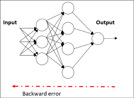
Figure 14.10: Backward step in backpropagation

The process of forward propagation from input to output and backward propagation of errors is repeated several times until the error goes below a predefined threshold. The whole process is represented in Figure 14.11. A set of features is selected as input to a machine learning model that produces predictions.

The predictions are compared with the (true) label, and the resulting loss function is minimized by the optimizer, which updates the weights of the model:

Figure 14.11: Forward propagation and backward propagation

Let’s see in detail how the forward and backward steps are realized. It might be useful to have a look back at Figure 14.5 and recall that a small change in a specific w_ij will be propagated through the network following its topology (see Figure 14.5, where the edges in bold are the ones impacted by the small change in specific weights).

Forward step

During the forward steps, the inputs are multiplied with the weights and then all summed together. Then the activation function is applied (see Figure 14.12). This step is repeated for each layer, one after another. The first layer takes the input features as input and it produces its output. Then, each subsequent layer takes as input the output of the previous layer:

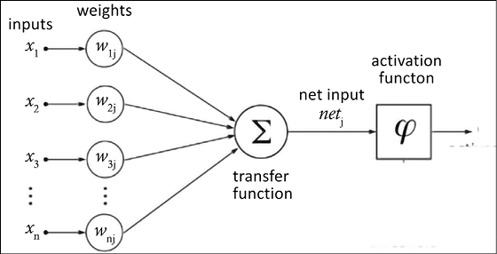
Figure 14.12: Forward propagation

If we look at one single layer, mathematically we have two equations:

• The transfer equation , where x_i are the input values, w_i are the weights, and b is the bias. In vector notation . Note that b can be absorbed in the summatory by setting and .
• The activation function: , where is the chosen activation function.

An artificial neural network consists of an input layer I, an output layer O, and any number of hidden layers H_i situated between the input and the output layers. For the sake of simplicity, let’s assume that there is only one hidden layer, since the results can be easily generalized.

As shown in Figure 14.12, the features x_i from the input layer are multiplied by a set of fully connected weights w_ij connecting the input layer to the hidden layer (see the left side of Figure 14.12). The weighted signals are summed together and with the bias to calculate the result (see the center of Figure 14.12). The result is passed through the activation function 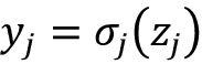, which leaves the hidden layer to the output layer (see the right side of Figure 14.12).

In summary, during the forward step we need to run the following operations:

1. For each neuron in a layer, multiply each input by its corresponding weight.
2. Then for each neuron in the layer, sum all input weights together.
3. Finally, for each neuron, apply the activation function on the result to compute the new output.

At the end of the forward step, we get a predicted vector from the output layer o given the input vector x presented at the input layer. Now the question is: how close is the predicted vector to the true value vector t?

That’s where the backstep comes in.

Backstep

To understand how close the predicted vector is to the true value vector t, we need a function that measures the error at the output layer o. That is the loss function defined earlier in the book. There are many choices for loss function. For instance, we can define the mean squared error defined as follows:

Note that E is a quadratic function and, therefore, the difference is quadratically larger when t is far away from , and the sign is not important. Note that this quadratic error (loss) function is not the only one that we can use. Later in this chapter, we will see how to deal with cross-entropy.

Now, remember that the key point is that during the training, we want to adjust the weights of the network to minimize the final error. As discussed, we can move toward a local minimum by moving in the opposite direction to the gradient . Moving in the opposite direction to the gradient is the reason why this algorithm is called gradient descent. Therefore, it is reasonable to define the equation for updating the weight w_ij as follows:

For a function in multiple variables, the gradient is computed using partial derivatives. We introduce the hyperparameter – or, in ML lingo, the learning rate – to account for how large a step should be in the direction opposite to the gradient.

Considering the error, E, we have the equation:

The preceding equation is simply capturing the fact that a slight change will impact the final error, as seen in Figure 14.13:

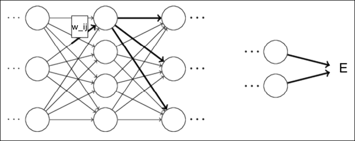
Figure 14.13: A small change in w_ij will impact the final error E

Let’s define the notation used throughout our equations in the remaining section:

• is the input to node j for layer l.
• is the activation function for node j in layer l (applied to ).
• is the output of the activation of node j in layer l.
• is the matrix of weights connecting the neuron i in layer to the neuron j in layer l.
• is the bias for unit j in layer l.
• is the target value for node o in the output layer.

Now we need to compute the partial derivative for the error at the output layer when the weights change by . There are two different cases:

• Case 1: Weight update equation for a neuron from hidden (or input) layer to output layer.
• Case 2: Weight update equation for a neuron from hidden (or input) layer to hidden layer.

We’ll begin with Case 1.

Case 1: From hidden layer to output layer

In this case, we need to consider the equation for a neuron from hidden layer j to output layer o. Applying the definition of E and differentiating we have:

Here the summation disappears because when we take the partial derivative with respect to the j-th dimension, the only term that is not zero in the error is the j-th. Considering that differentiation is a linear operation and that – because the true value does not depend on – we have:

Applying the chain rule again and remembering that , we have:

Remembering that , we have again because when we take the partial derivative with respect to the j-th dimension the only term that is not zero in the error is the j-th. By definition , so putting everything together we have:

The gradient of the error E with respect to the weights w_j from the hidden layer j to the output layer o is therefore simply the product of three terms: the difference between the prediction and the true value , the derivative of the output layer activation function, and the activation output of node j in the hidden layer. For simplicity we can also define and get:

In short, for Case 1, the weight update equation for each of the hidden-output connections is:

Note: if we want to explicitly compute the gradient with respect to the output layer biases, the steps to follow are similar to the ones above with only one difference:

so in this case .

Next, we’ll look at Case 2.

Case 2: From hidden layer to hidden layer

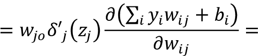
In this case, we need to consider the equation for a neuron from a hidden layer (or the input layer) to a hidden layer. Figure 14.13 showed that there is an indirect relationship between the hidden layer weight change and the output error. This makes the computation of the gradient a bit more challenging. In this case, we need to consider the equation for a neuron from hidden layer i to hidden layer j.

Applying the definition of E and differentiating we have:

In this case, the sum will not disappear because the change of weights in the hidden layer is directly affecting the output. Substituting and applying the chain rule we have:

The indirect relation between and the internal weights w_ij (Figure 14.13) is mathematically expressed by the expansion:

since .

This suggests applying the chain rule again:

Applying the chain rule:

Substituting :

Deriving:

Substituting :

Applying the chain rule:

Substituting :

Deriving:

Now we can combine the above two results:

and get:

Remembering the definition: , we get:

This last substitution with is particularly interesting because it backpropagates the signal computed in the subsequent layer. The rate of change with respect to the rate of change of the weights w_ij is therefore the multiplication of three factors: the output activations y_i from the layer below, the derivative of hidden layer activation function , and the sum of the backpropagated signal previously computed in the subsequent layer weighted by . We can use this idea of backpropagating the error signal by defining and therefore . This suggests that in order to calculate the gradients at any layer in a deep neural network, we can simply multiply the backpropagated error signal and multiply it by the feed-forward signal , arriving at the layer l. Note that the math is a bit complex but the result is indeed very very simple! The intuition is given in Figure 14.14. Given a function , computed locally to a neuron with the input , and , the gradients are backpropagated. Then, they are combined via the chain rule with the local gradients and for further backpropagation.

Here, L denotes the error from the generic previous layer:

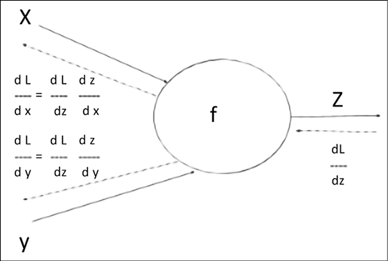
Figure 14.14: An example of the math behind backpropagation

Note: if we want to explicitly compute the gradient with respect to the output layer biases, it can be proven that 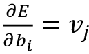. We leave this as an exercise for you.

In short, for Case 2 (hidden-to-hidden connection) the weight delta is and the weight update equation for each of the hidden-hidden connections is simply:

We have arrived at the end of this section and all the mathematical tools are defined to make our final statement. The essence of the backstep is nothing more than applying the weight update rule one layer after another, starting from the last output layer and moving back toward the first input layer. Difficult to derive, to be sure, but extremely easy to apply once defined. The whole forward-backward algorithm at the core of deep learning is then the following:

1. Compute the feedforward signals from the input to the output.
2. Compute the output error E based on the predictions and the true value .
3. Backpropagate the error signals; multiply them with the weights in previous layers and with the gradients of the associated activation functions.
4. Compute the gradients for all of the parameters based on the backpropagated error signal and the feedforward signals from the inputs.
5. Update the parameters using the computed gradients .

Note that the above algorithm will work for any choice of differentiable error function E and for any choice of differentiable activation function. The only requirement is that both must be differentiable.

Gradient descent with backpropagation is not guaranteed to find the global minimum of the loss function, but only a local minimum. However, this is not necessarily a problem observed in practical application.

Cross entropy and its derivative

Gradient descent can be used when cross-entropy is adopted as the loss function. As discussed in Chapter 1, Neural Network Foundations with TF, the logistic loss function is defined as:

Where c refers to one-hot-encoded classes (or labels) whereas p refers to softmax-applied probabilities. Since cross-entropy is applied to softmax-applied probabilities and to one-hot-encoded classes, we need to take into account the chain rule for computing the gradient with respect to the final weights score_i. Mathematically, we have:

Computing each part separately, let’s start from :

(noting that for a fixed all the terms in the sum are constant except the chosen one).

Therefore, we have:

(applying the partial derivative to the sum and considering that )

Therefore, we have:

Now let’s compute the other part where p_i is the softmax function defined as:

The derivative is:

and

Using the Kronecker delta we have:

Therefore, considering that we are computing the partial derivative, all the components are zeroed with the exception of only one, and we have:

Combining the results, we have:

Where c_i denotes the one-hot-encoded classes and p_i refers to the softmax probabilities. In short, the derivative is both elegant and easy to compute:

Batch gradient descent, stochastic gradient descent, and mini-batch

If we generalize the previous discussion, then we can state that the problem of optimizing a neural network consists of adjusting the weights w of the network in such a way that the loss function is minimized. Conveniently, we can think about the loss function in the form of a sum, as in this form it’s indeed representing all the loss functions commonly used:

In this case, we can perform a derivation using steps very similar to those discussed previously, following the update rule, where is the learning rate and is the gradient:

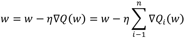
In many cases, evaluating the above gradient might require an expensive evaluation of the gradients from all summand functions. When the training set is very large, this can be extremely expensive. If we have three million samples, we have to loop through three million times or use the dot product. That’s a lot! How can we simplify this? There are three types of gradient descent, each different in the way they handle the training dataset.

Batch gradient descent

Batch Gradient Descent (BGD) computes the change of error but updates the whole model only once the entire dataset has been evaluated. Computationally it is very efficient, but it requires that the results for the whole dataset be held in the memory.

Stochastic gradient descent

Instead of updating the model once the dataset has been evaluated, Stochastic Gradient Descent (SGD) does so after every single training example. The key idea is very simple: SGD samples a subset of summand functions at every step.

Mini-batch gradient descent

Mini-Batch Gradient Descent (MBGD) is very frequently used in deep learning. MBGD (or mini-batch) combines BGD and SGD in one single heuristic. The dataset is divided into small batches of about size bs, generally 64 to 256. Then each of the batches is evaluated separately.

Note that bs is another hyperparameter to fine-tune during training. MBGD lies between the extremes of BGD and SGD – by adjusting the batch size and the learning rate parameters, we sometimes find a solution that descends closer to the global minimum than what can be achieved by either of the extremes.

In contrast with gradient descent, where the cost function is minimized more smoothly, the mini-batch gradient has a bit more of a noisy and bumpy descent, but the cost function still trends downhill. The reason for the noise is that mini-batches are a sample of all the examples and this sampling can cause the loss function to oscillate.

Thinking about backpropagation and ConvNets

In this section, we will examine backprop and ConvNets. For the sake of simplicity, we will focus on an example of convolution with input X of size 3x3, one single filter W of size 2x2 with no padding, stride 1, and no dilation (see Chapter 3, Convolutional Neural Networks). The generalization is left as an exercise.

The standard convolution operation is represented in Figure 14.15. Simply put, the convolutional operation is the forward pass:

Input X11 X12 X13 X21 X22 X23 X31 X32 X33

Weights W11 W12 W21 W22

Convolution W11X11+W12X12+W21X21+W22X22 W11X12+W12X13+W21X21+W22X23 W11X21+W12X22+W21X31+W22X32 W11X22+W12X23+W21X32+W22X33

Figure 14.15: Forward pass for our ConvNet toy example

Following the examination of Figure 14.15, we can now focus our attention on the backward pass for the current layer. The key assumption is that we receive a backpropagated signal as input, and we need to compute and . This computation is left as an exercise, but please note that each weight in the filter contributes to each pixel in the output map or, in other words, any change in a weight of a filter affects all the output pixels.

Thinking about backpropagation and RNNs

Remember from Chapter 5, Recurrent Neural Networks, the basic equation for an RNN is , the final prediction is at step t, the correct value is y_t, and the error E is the cross-entropy. Here U, V, and W are learning parameters used for the RNN’s equations. These equations can be visualized as shown in Figure 14.16, where we unroll the recurrency. The core idea is that total error is just the sum of the errors at each time step.

If we used SGD, we need to sum the errors and the gradients at each time step for one given training example:

Figure 14.16: RNN unrolled with equations

We are not going to write all the tedious math behind all the gradients but rather focus only on a few peculiar cases. For instance, with math computations similar to the ones made in the previous sections, it can be proven by using the chain rule that the gradient for V depends only on the value at the current time step s₃, y₃ and :

However, has dependencies carried across time steps because, for instance, depends on s₂, which depends on W₂ and s₁. As a consequence, the gradient is a bit more complicated because we need to sum up the contributions of each time step:

To understand the preceding equation, imagine that we are using the standard backpropagation algorithm used for traditional feedforward neural networks but for RNNs. We need to additionally add the gradients of W across time steps. That’s because we can effectively make the dependencies across time explicit by unrolling the RNN. This is the reason why backprop for RNNs is frequently called Backpropagation Through Time (BPTT).

The intuition is shown in Figure 14.17, where the backpropagated signals are represented:

Figure 14.17: RNN equations and backpropagated signals

I hope that you have been following up to this point because now the discussion will be slightly more difficult. If we consider:

then we notice that should be again computed with the chain rule, producing a number of multiplications. In this case, we take the derivative of a vector function with respect to a vector, so we need a matrix whose elements are all the pointwise derivatives (in math, this matrix is called a Jacobian). Mathematically, it can be proven that:

Therefore, we have:

The multiplication in the above equation is particularly problematic since both the sigmoid and tanh get saturated at both ends and their derivative goes to 0. When this happens, they drive other gradients in previous layers toward 0. This makes the gradient vanish completely after a few time steps and the network stops learning from “far away.”

Chapter 5, Recurrent Neural Networks, discussed how to use Long Short-Term Memory (LSTM) and Gated Recurrent Units (GRUs) to deal with the problem of vanishing gradients and efficiently learn long-range dependencies. In a similar way, the gradient can explode when one single term in the multiplication of the Jacobian matrix becomes large. Chapter 5 discussed how to use gradient clipping to deal with this problem.

We have now concluded this journey, and you should now understand how backpropagation works and how it is applied in neural networks for dense networks, CNNs, and RNNs. In the next section, we will discuss how TensorFlow computes gradients, and why this is useful for backpropagation.

A note on TensorFlow and automatic differentiation

TensorFlow can automatically calculate derivatives, a feature called automatic differentiation. This is achieved by using the chain rule. Every node in the computational graph has an attached gradient operation for calculating the derivatives of input with respect to output. After that, the gradients with respect to parameters are automatically computed during backpropagation.

Automatic differentiation is a very important feature because you do not need to hand-code new variations of backpropagation for each new model of a neural network. This allows for quick iteration and running many experiments faster.

Summary

In this chapter, we discussed the math behind deep learning. Put simply, a deep learning model computes a function given an input vector to produce the output. The interesting part is that it can literally have billions of parameters (weights) to be tuned. Backpropagation is a core mathematical algorithm used by deep learning for efficiently training artificial neural networks, following a gradient descent approach that exploits the chain rule. The algorithm is based on two steps repeated alternatively: the forward step and the backstep.

During the forward step, inputs are propagated through the network to predict the outputs. These predictions might be different from the true values given to assess the quality of the network. In other words, there is an error and our goal is to minimize it. This is where the backstep plays a role, by adjusting the weights of the network to minimize the error. The error is computed via loss functions such as Mean Squared Error (MSE), or cross-entropy for non-continuous values such as Boolean (Chapter 1, Neural Network Foundations with TF). A gradient-descent-optimization algorithm is used to adjust the weight of neurons by calculating the gradient of the loss function. Backpropagation computes the gradient, and gradient descent uses the gradients for training the model. A reduction in the error rate of predictions increases accuracy, allowing machine learning models to improve. SGD is the simplest thing you could possibly do by taking one step in the direction of the gradient. This chapter does not cover the math behind other optimizers such as Adam and RMSProp (Chapter 1). However, they involve using the first and the second moments of the gradients. The first moment involves the exponentially decaying average of the previous gradients, and the second moment involves the exponentially decaying average of the previous squared gradients.

There are three big properties of our data that justify using deep learning; otherwise, we might as well use regular machine learning:

• Very-high-dimensional input (text, images, audio signals, videos, and temporal series are frequently a good example).
• Dealing with complex decision surfaces that cannot be approximated with a low-order polynomial function.
• Having a large amount of training data available.

Deep learning models can be thought of as a computational graph made up of stacking together several basic components such as dense networks (Chapter 1), CNNs (Chapter 3), embeddings (Chapter 4), RNNs (Chapter 5), GANs (Chapter 9), autoencoders (Chapter 8) and, sometimes, adopting shortcut connections such as “peephole,” “skip,” and “residual” because they help data flow a bit more smoothly. Each node in the graph takes tensors as input and produces tensors as output. As discussed, training happens by adjusting the weights in each node with backprop, where the key idea is to reduce the error in the final output node(s) via gradient descent. GPUs and TPUs (Chapter 15) can significantly accelerate the optimization process since it is essentially based on (hundreds of) millions of matrix computations.

There are a few other mathematical tools that might be helpful to improve your learning process. Regularization (L1, L2, and Lasso (Chapter 1)) can significantly improve learning by keeping weights normalized. Batch normalization (Chapter 1) helps to basically keep track of the mean and the standard deviation of your dataset across multiple deep layers. The key idea is to have data resembling a normal distribution while it flows through the computational graph. Dropout (Chapters 1, 3, 5, 6, 9, and 20) helps by introducing some elements of redundancy in your computation; this prevents overfitting and allows better generalization.

This chapter has presented the mathematical foundation behind intuition. As discussed, this topic is quite advanced and not necessarily required for practitioners. However, it is recommended reading if you are interested in understanding what is going on “under the hood” when you play with neural networks.

The next chapter will introduce the Tensor Processing Unit (TPU), a special chip developed at Google for ultra-fast execution of many mathematical operations described in this chapter.

References

1. Kelley, Henry J. (1960). Gradient theory of optimal flight paths. ARS Journal. 30 (10): 947–954. Bibcode:1960ARSJ...30.1127B. doi:10.2514/8.5282.
2. Dreyfus, Stuart. (1962). The numerical solution of variational problems. Journal of Mathematical Analysis and Applications. 5 (1): 30–45. doi:10.1016/0022-247x(62)90004-5.
3. Werbos, P. (1974). Beyond Regression: New Tools for Prediction and Analysis in the Behavioral Sciences. PhD thesis, Harvard University.
4. Rumelhart, David E.; Hinton, Geoffrey E.; Williams, Ronald J. (1986-10-09). Learning representations by back-propagating errors. Nature. 323 (6088): 533–536. Bibcode:1986Natur.323..533R. doi:10.1038/323533a0.
5. LeCun, Y. (1987). Modèles Connexionnistes de l’apprentissage (Connectionist Learning Models), Ph.D. thesis, Université P. et M. Curie.
6. Herbert Robbins and Sutton Monro. (1951). A Stochastic Approximation Method. The Annals of Mathematical Statistics, Vol. 22, No. 3. pp. 400–407.
7. Krizhevsky, Alex; Sutskever, Ilya; Hinton, Geoffrey E. (June 2017). ImageNet classification with deep convolutional neural networks (PDF). Communications of the ACM. 60 (6): 84–90. doi:10.1145/3065386. ISSN 0001-0782.
8. From not working to neural networking. The Economist. (25 June 2016)

Join our book’s Discord space

Join our Discord community to meet like-minded people and learn alongside more than 2000 members at: https://packt.link/keras