16

Other Useful Deep Learning Libraries

TensorFlow from Google is not the only framework available for deep learning tasks. There is a good range of libraries and frameworks available, each with its special features, capabilities, and use cases. In this chapter, we will explore some of the popular deep learning libraries and compare their features.

The chapter will include:

• Hugging Face
• H2O
• PyTorch
• ONNX
• Open AI

Let’s begin!

Hugging Face

Hugging Face is not new for us; Chapter 6, Transformers, introduced us to the library. Hugging Face is an NLP-centered startup, founded by Delangue and Chaumond in 2016. It has, in a short time, established itself as one of the best tools for all NLP-related tasks. The AutoNLP and accelerated inference API are available for a price. However, its core NLP libraries datasets, tokenizers, Accelerate, and transformers (Figure 16.1) are available for free. It has built a cool community-driven open-source platform.

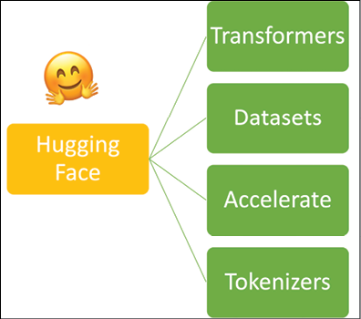
Figure 16.1: NLP libraries from Hugging Face

The core of the Hugging Face ecosystem is its transformers library. The Tokenizers and Datasets libraries support the Transformers library. To use these libraries, we need to install them first. Transformers can be installed using a simple pip install command:

pip install transformers

Some of the out-of-the-box models available with Hugging Face are text summarization, question answering, text classification, audio classification, automatic speech recognition, feature extraction, image classification, and translation. In Figure 16.2, we can see the result of the out-of-the-box summarization model available with Hugging Face.

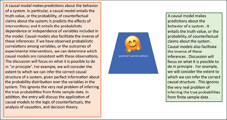
Figure 16.2: Out-of-the-box text summarization using Hugging Face

Besides these out-of-the-box models, we can use the large number of models and datasets available at Hugging Face Hub and can use them with PyTorch, TensorFlow, and JAX to build customized models.

OpenAI

OpenAI is another well-known name for people working in the field of reinforcement learning. Their Gym module is a standard toolkit used by developers across the globe for developing and comparing reinforcement learning algorithms. In Chapter 11, Reinforcement Learning, we have already covered the Gym module in detail. In this chapter, we will explore two more offerings by OpenAI.

OpenAI GPT-3 API

“OpenAI GPT3 is a machine learning platform that allows developers to build custom algorithms for deep learning. This platform was released in December of 2017 and has been widely used by businesses and individuals in the field of artificial intelligence. One of the primary reasons that GPT3 has been so successful is because it is easy to use and has a wide range of features. This platform is able to learn from data and can be used for a variety of tasks, including deep learning, natural language processing, and image recognition. GPT3 is also popular because it is open source and can be used by anyone. This makes it an ideal platform for anyone who wants to learn about deep learning and the various ways that it can be used. Overall, GPT3 is a powerful and easy-to-use machine learning platform that has been widely used by businesses and individuals in the field of artificial intelligence.”

This is the text generated by the OpenAI GPT-3 API, when asked to write on GPT-3 itself (https://beta.openai.com/playground):

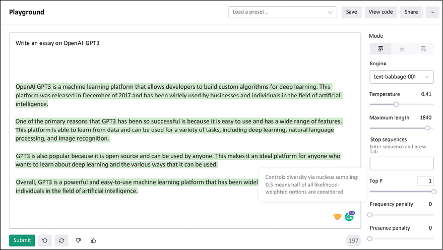
Figure 16.3: Text generation using OpenAI GPT-3 API

The OpenAI GPT-3 API offers the following tasks:

• Text Completion: Here, the GPT-3 API is used to generate or manipulate text and even code. You can use it to write a tagline, an introduction, or an essay, or you can leave a sentence half-written and ask it to complete it. People have used it to generate stories and advertisement leads.
• Semantic Search: This allows you to do a semantic search over a set of documents. For example, you can upload documents using the API; it can handle up to 200 documents, where each file can be a maximum of 150 MB in size, and the total limited to 1 GB at any given time. The API will take your query and rank the documents based on the semantic similarity score (ranges normally between 0-300).
• Question Answering: This API uses the documents uploaded as the source of truth; the API first searches the documents for relevance to the question. Then it ranks them based on the semantic relevance and finally, answers the question.
• Text Classification: The text classification endpoint of OpenAI GPT-3 takes as input a labeled set of examples and then uses the labels in it to label the query text. There are a lot of examples where this feature has been used to perform sentiment analysis.

Initially, the OpenAI GPT-3 was available only after applying for it, but now, anyone can use the API; there is no longer a waitlist.

OpenAI DALL-E 2

The GPT-3 API by OpenAI deals with all things related to NLP; DALL-E 2 goes a step further. DALL-E was originally released by OpenAI in January 2021. It claims to produce photorealistic images based on the textual description provided to the model. It can also make realistic edits to existing images; you can use it to add or remove objects and elements from the image, and when it does so, it considers the effect on shadows, reflections, and texture. Figure 16.4 shows some of the remarkable feats by DALL-E 2. In the figures on the top row, I gave DALL-E 2 a text describing what I want: “Albert Einstein flying on dinosaur over the Amazon Forest.” It generated a cartoon-like image. The images in the lower row are generated using the image-editor feature of DALL-E 2. I added the image on the left, and it generated four variations. The variations look very realistic if you ignore that the faces are blurred:

Figure 16.4: On top is the image generated by DALL-E 2, and below are the images edited by DALL-E 2

At the time of writing this book (August 2022), DALL-E 2 is not available for public use. But imagine the possibilities for artists and professionals working in creating digital media once the model is available as an API.

OpenAI Codex

When a student starts with their first lessons of programming, as a teacher, I often recommend that they think of a program as a set of instructions – the only important thing to master is writing those instructions as clearly as possible in whatever language you know.

Well, Codex makes it happen, you just need to give it the instructions of what you want to achieve, and it will generate the respective code for you.

OpenAI launches it as a general-purpose programming model, and it has been trained on publicly available GitHub codes.

Below are a few snippets of the task and corresponding code generated by Codex:

""" Ask the user for their name and say "Hello" in Python """ 
print("Hello, world!") 
name = input("Please type your name: ") 
print("Hello, " + name + "!")
""" Write a program in Python to find sum of n fibonacci sequences """ 
def Fibonacci(n): 
    if n < 0: 
        print("Incorrect input") 
    elif n == 1: 
       return 0 
    elif n == 2: 
        return 1 
    else: 
        return Fibonacci(n - 1) + Fibonacci(n - 2) 
n = int(input("Enter the number of terms: ")) 
# check if the number of terms is valid 
if n <= 0: 
    print("Please enter a positive integer") 
else: 
    print("Fibonacci sequence: ") 
    for I in range(1, n + 1): 
        print(Fibonacci(n), end=' ')

The first task, as you can see, is done flawlessly. In the second task, we asked it to find the sum of the Fibonacci sequence; instead, it generated the Fibonacci sequence, which is a more common problem. This tells us that while it is great at doing run-of-the-mill jobs, the need for real programmers is still there.

PyTorch

Like TensorFlow, PyTorch is a full-fledged deep learning framework. In AI-based social groups, you will often find die-hard fans of PyTorch and TensorFlow arguing that theirs is best. PyTorch, developed by Facebook (Meta now), is an open-source deep learning framework. Many researchers prefer it for its flexible and modular approach. PyTorch also has stable support for production deployment. Like TF, the core of PyTorch is its tensor processing library and its automatic differentiation engine. In a C++ runtime environment, it leverages TorchScript for an easy transition between graph and eager mode. The major feature that makes PyTorch popular is its ability to use dynamic computation, i.e., its ability to dynamically build the computational graph – this gives the programmer flexibility to modify and inspect the computational graphs anytime.

The PyTorch library consists of many modules, which are used as building blocks to make complex models. Additionally, PyTorch also provides convenient functions to transfer variables and models between different devices viz CPU, GPU, or TPU. Of special mention are the following three powerful modules:

• NN Module: This is the base class where all layers and functions to build a deep learning network are. Below, you can see the code snippet where the NN module is used to build a network. The network can then be instantiated using the statement net = My_Net(1,10,5); this creates a network with one input channel, 10 output neurons, and a kernel of size 5x5:

  import torch.nn as nn
  import torch.nn.functional as F
  class My_Net(nn.Module):
      def __init__(self, input_channel, output_neurons, kernel_size):
          super(My_Net, self).__init__()
          self.conv1 = nn.Conv2d(input_channel, 6, kernel_size)
          self.conv2 = nn.Conv2d(6, 16, 5)
          self.fc1 = nn.Linear(16 * 5 * 5, 120)
          self.fc2 = nn.Linear(120, 84)
          self.fc3 = nn.Linear(84,output_neurons)
      def forward(self, x):
          x = F.max_pool2d(F.relu(self.conv1(x)), (2, 2))
          x = F.max_pool2d(F.relu(self.conv2(x)), 2)
          x = x.view(-1, self.num_flat_features(x))
          x = F.relu(self.fc1(x))
          x = F.relu(self.fc2(x))
          x = self.fc3(x)
          return x
      def num_flat_features(self, x):
          size = x.size()[1:]  
          num_features = 1
          for s in size:
              num_features *= s
          return num_features
  

  Here is a summary of the network:

  My_Net(
      (conv1): Conv2d(1, 6, kernel_size=(5, 5), stride=(1, 1))
      (conv2): Conv2d(6, 16, kernel_size=(5, 5), stride=(1,
      1))
      (fc1): Linear(in_features=400, out_features=120,
      bias=True)
      (fc2): Linear(in_features=120, out_features=84,
      bias=True)
      (fc3): Linear(in_features=84, out_features=10,
      bias=True)
  )
  

• Autograd Module: This is the heart of PyTorch. The module provides classes and functions that are used for implementing automatic differentiation. The module creates an acyclic graph called the dynamic computational graph; the leaves of this graph are the input tensors, and the root is the output tensors. It calculates a gradient by tracing the root to the leaf and multiplying every gradient in the path using the chain rule. The following code snippet shows how to use the Autograd module for calculating gradients. The backward() function computes the gradient of the loss with respect to all the tensors whose requires_grad is set to True. So suppose you have a variable w, then after the call to backward(), the tensor w.grad will give us the gradient of the loss with respect to w.

  We can then use this to update the variable w as per the learning rule:

  loss = (y_true – y_pred).pow(2).sum()
  loss.backward()
  # Here the autograd is used to compute the backward pass. 
  With torch.no_grad():
      W = w – lr_rate * w.grad
      w.grad = None # Manually set to zero after updating
  

• Optim Module: The Optim module implements various optimization algorithms. Some of the optimizer algorithms available in Optim are SGD, AdaDelta, Adam, SparseAdam, AdaGrad, and LBFGS. One can also use the Optim module to create complex optimizers. To use the Optim module, one just needs to construct an optimizer object that will hold the current state and will update the parameters based on gradients.

PyTorch is used by many companies for their AI solutions. Tesla uses PyTorch for AutoPilot. The Tesla Autopilot, which uses the footage from eight cameras around the vehicle, passes that footage through 48 neural networks for object detection, semantic segmentation, and monocular depth estimation. The system provides level 2 vehicle automation. They take video from all eight cameras to generate road layout, any static infrastructure (e.g., buildings and traffic/electricity poles), and 3D objects (other vehicles, persons on the road, and so on). The networks are trained iteratively in real time. While a little technical, this 2019 talk by Andrej Karpathy, Director of AI at Tesla, gives a bird’s-eye view of Autopilot and its capabilities: https://www.youtube.com/watch?v=oBklltKXtDE&t=670s. Uber’s Pyro, a probabilistic deep learning library, and OpenAI are other examples of big AI companies using PyTorch for research and development.

ONNX

Open Neural Network Exchange (ONNX) provides an open-source format for AI models. It supports both deep learning models and traditional machine learning models. It is a format designed to represent any type of model, and it achieves this by using an intermediate representation of the computational graph created by different frameworks. It supports PyTorch, TensorFlow, MATLAB, and many more deep learning frameworks. Thus, using ONNX, we can easily convert models from one framework to another. This helps in reducing the time from research to deployment. For example, you can use ONNX to convert a PyTorch model to ONNX.js form, which can then be directly deployed on the web.

H2O.ai

H2O is a fast, scalable machine learning and deep learning framework developed by H2O.ai, released under the open-source Apache license. According to the company website, as of the time of writing this book, more than 20,000 organizations use H2O for their ML/deep learning needs. The company offers many products like H2O AI cloud, H2O Driverless AI, H2O wave, and Sparkling Water. In this section, we will explore its open-source product, H2O.

It works on big data infrastructure on Hadoop, Spark, or Kubernetes clusters and it can also work in standalone mode. It makes use of distributed systems and in-memory computing, which allows it to handle a large amount of data in memory, even with a small cluster of machines. It has an interface for R, Python, Java, Scala, and JavaScript, and even has a built-in web interface.

H2O includes a large number of statistical-based ML algorithms such as generalized linear modeling, Naive Bayes, random forest, gradient boosting, and all major deep learning algorithms. The best part of H2O is that one can build thousands of models, compare the results, and even do hyperparameter tuning with only a few lines of code. H2O also has better data pre-processing tools.

H2O requires Java, therefore, ensure that Java is installed on your system. You can install H2O to work in Python using PyPi, as shown in the following code:

pip install h2o

H2O AutoML

One of the most exciting features of H2O is AutoML, the automatic ML. It is an attempt to develop a user-friendly ML interface that can be used by beginners and non-experts. H2O AutoML automates the process of training and tuning a large selection of candidate models. Its interface is designed so that users just need to specify their dataset, input and output features, and any constraints they want on the number of total models trained, or time constraints. The rest of the work is done by the AutoML itself, in the specified time constraint; it identifies the best performing models and provides a leaderboard. It has been observed that usually, the Stacked Ensemble model, the ensemble of all the previously trained models, occupies the top position on the leaderboard. There is a large number of options that advanced users can use; details of these options and their various features are available at http://docs.h2o.ai/h2o/latest-stable/h2o-docs/automl.html.

To learn more about H2O, visit their website: http://h2o.ai.

AutoML using H2O

Let us try H2O AutoML on a synthetically created dataset. We use the scikit-learn make_circles method to create the data and save it as a CSV file:

from sklearn.datasets import make_circles
import pandas as pd
X, y = make_circles(n_samples=1000, noise=0.2, factor=0.5, random_state=9)
df = pd.DataFrame(X, columns=['x1','x2'])
df['y'] = y
df.head()
df.to_csv('circle.csv', index=False, header=True)

Before we can use H2O, we need to initiate its server, which is done using the init() function:

import h2o
h2o.init()

The following shows the output we will receive after initializing the H2O server:

Checking whether there is an H2O instance running at http://localhost:54321 ..... not found.
Attempting to start a local H2O server...
  Java Version: openjdk version "11.0.15" 2022-04-19; OpenJDK Runtime Environment (build 11.0.15+10-Ubuntu-0ubuntu0.18.04.1); OpenJDK 64-Bit Server VM (build 11.0.15+10-Ubuntu-0ubuntu0.18.04.1, mixed mode, sharing)
  Starting server from /usr/local/lib/python3.7/dist-packages/h2o/backend/bin/h2o.jar
  Ice root: /tmp/tmpm2fsae68
  JVM stdout: /tmp/tmpm2fsae68/h2o_unknownUser_started_from_python.out
  JVM stderr: /tmp/tmpm2fsae68/h2o_unknownUser_started_from_python.err
  Server is running at http://127.0.0.1:54321
Connecting to H2O server at http://127.0.0.1:54321 ... successful.
H2O_cluster_uptime:    05 secs
H2O_cluster_timezone:    Etc/UTC
H2O_data_parsing_timezone:    UTC
H2O_cluster_version:    3.36.1.1
H2O_cluster_version_age:    27 days 
H2O_cluster_name:    H2O_from_python_unknownUser_45enk6
H2O_cluster_total_nodes:    1
H2O_cluster_free_memory:    3.172 Gb
H2O_cluster_total_cores:    2
H2O_cluster_allowed_cores:    2
H2O_cluster_status:    locked, healthy
H2O_connection_url:    http://127.0.0.1:54321
H2O_connection_proxy:    {"http": null, "https": null}
H2O_internal_security:    False
Python_version:    3.7.13 final

We read the file containing the synthetic data that we created earlier. Since we want to treat the problem as a classification problem, whether the points lie in a circle or not, we redefine our label 'y' as asfactor() – this will tell the H2O AutoML module to treat the variable y as categorical, and thus the problem as classification. The dataset is split into training, validation, and test datasets in a ratio of 60:20:20:

class_df = h2o.import_file("circle.csv",
                           destination_frame="circle_df")
class_df['y'] = class_df['y'].asfactor()
train_df,valid_df,test_df = class_df.split_frame(ratios=[0.6, 0.2],
                                                 seed=133)

And now we invoke the AutoML module from H2O and train on our training dataset. AutoML will search a maximum of 10 models, but you can change the parameter max_models to increase or decrease the number of models to test:

from h2o.automl import H2OAutoML as AutoML
aml = AutoML(max_models = 10, max_runtime_secs=100, seed=2)
aml.train(training_frame= train_df, 
          validation_frame=valid_df, 
          y = 'y', x=['x1','x2'])

For each of the models, it gives a performance summary, for example, in Figure 16.5, you can see the evaluation summary for a binomial GLM:

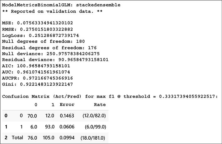
Figure 16.5: Performance summary of one of the models by H2O AutoML

You can check the performance of all the models evaluated by H2O AutoML on a leaderboard:

lb = aml.leaderboard
lb.head()

Here is the snippet of the leaderboard:

model_id     auc    logloss    aucpr    mean_per_class_error    rmse    mse
StackedEnsemble_BestOfFamily_1_AutoML_2_20220511_61356    0.937598    0.315269    0.940757    0.117037    0.309796    0.0959735
StackedEnsemble_AllModels_1_AutoML_2_20220511_61356     0.934905    0.323695    0.932648    0.120348    0.312413    0.0976021
XGBoost_2_AutoML_2_20220511_61356     0.93281     0.322668    0.938299    0.122004    0.313339    0.0981811
XGBoost_3_AutoML_2_20220511_61356     0.932392    0.330866    0.929846    0.130168    0.319367    0.101995 
GBM_2_AutoML_2_20220511_61356     0.926839    0.353181    0.923751    0.141713    0.331589    0.109951 
XRT_1_AutoML_2_20220511_61356     0.925743    0.546718    0.932139    0.154774    0.331096    0.109625 
GBM_3_AutoML_2_20220511_61356     0.923935    0.358691    0.917018    0.143374    0.334959    0.112197 
DRF_1_AutoML_2_20220511_61356     0.922535    0.705418    0.921029    0.146669    0.333494    0.111218 
GBM_4_AutoML_2_20220511_61356     0.921954    0.36403     0.911036    0.151582    0.336908    0.113507 
XGBoost_1_AutoML_2_20220511_61356     0.919142    0.365454    0.928126    0.130227    0.336754    0.113403

H2O model explainability

H2O provides a convenient wrapper for a number of explainability methods and their visualizations using a single function explain() with a dataset and model. To get explainability on our test data for the models tested by AutoML, we will use aml.explain(). Below, we use the explain module for the StackedEnsemble_BestOfFamily model – the topmost in the leaderboard (we are continuing with the same data that we created in the previous section):

exa = aml.leader.explain(test_df)

The results are:

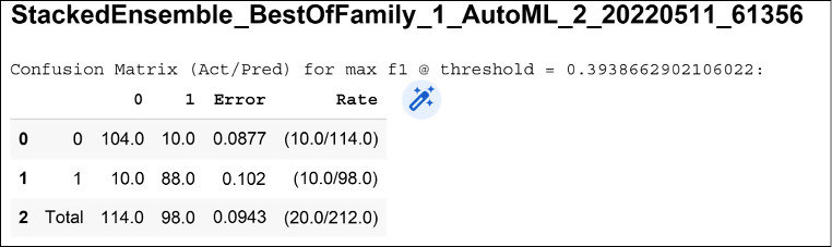
Figure 16.6: A confusion matrix on test dataset generated by H2O explain module

The ground truth is displayed in rows and the prediction by the model in columns. For our data, 0 was predicted correctly 104 times, and 1 was predicted correctly 88 times.

Partial dependence plots

Partial Dependence Plots (PDP) provide a graphical depiction of the marginal effect of a variable on the response of the model. It can tell us about the relationship between the output label and the input feature. Figure 16.7 shows the PDP plots as obtained from the H2O explain module on our synthetic dataset:

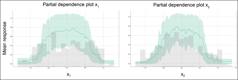
Figure 16.7: PDP for input features x₁ and x₂

For building PDP plots for each feature, H2O considers the rest of the features as constant. So, in the PDP plot for x₁ (x₂), the feature x₂ (x₁) is kept constant and the mean response is measured, as x₁ (x₂) is varied. The graph shows that both features play an important role in determining if the point is a circle or not, especially for values lying between [-0.5, 0.5].

Variable importance heatmap

We can also check the importance of variables across different models:

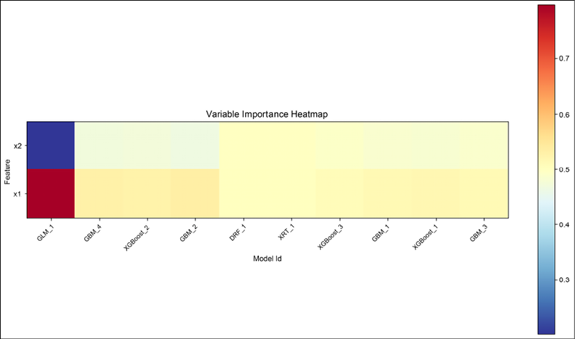
Figure 16.8: Variable importance heatmap for input features x₁ and x₂

Figure 16.8 shows how much importance was given to the two input features by different algorithms. We can see that the models that gave almost equal importance to the two features are doing well on the leaderboard, while GLM_1, which treated both features quite differently, has only about 41% accuracy.

Model correlation

The prediction between different models is correlated; we can check this correlation:

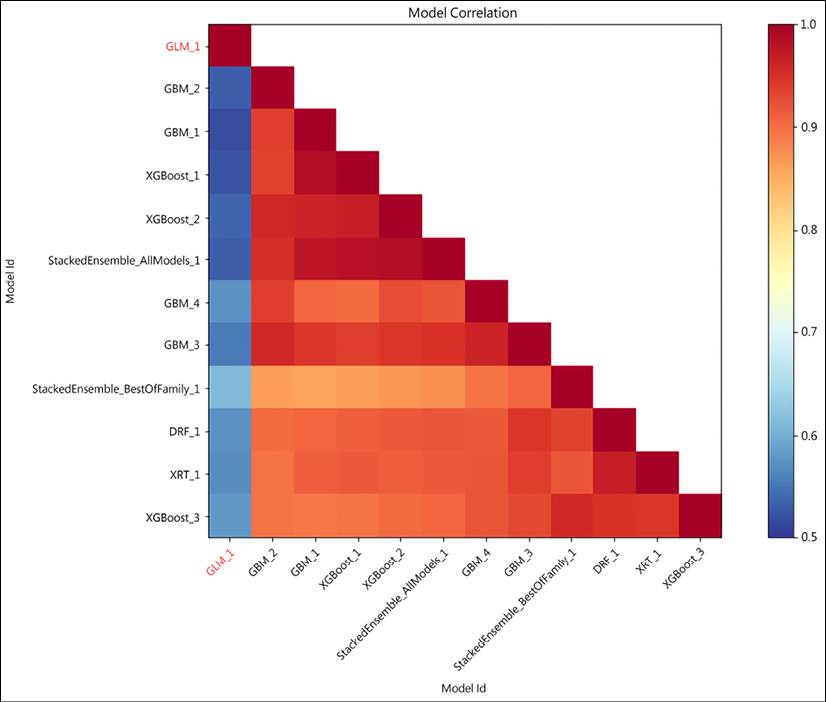
Figure 16.9: Model correlation

Figure 16.9 shows the model correlation; it shows the correlation between the predictions on the test dataset for different models. It measures the frequency of identical predictions to calculate correlations. Again, we can see that except for GLM_1, most other models perform almost equally, with accuracy ranging from 84-93% on the leaderboard.

What we have discussed here is just the tip of the iceberg; each of the frameworks listed here has entire books on their features and applications. Depending upon your use case, you should choose the respective framework. If you are building a model for production, TensorFlow is a better choice for both web-based and Edge applications. If you are building a model where you need better control of training and how the gradients are updated, then PyTorch is better suited. If you need to work cross-platform very often, ONNX can be useful. And finally, H2O and platforms like OpenAI GPT-3 and DALL-E 2 provide a low-threshold entry into the field of artificial intelligence and deep learning.

Summary

In this chapter, we briefly covered the features and capabilities of some other popular deep learning frameworks, libraries, and platforms. We started with Hugging Face, a popular framework for NLP. Then we explored OpenAI’s GPT-3 and DALL-E 2, both very powerful frameworks. The GPT-3 API can be used for a variety of NLP-related tasks, and DALL-E 2 uses GPT-3 to generate images from textual descriptions. Next, we touched on the PyTorch framework. According to many people, PyTorch and TensorFlow are equal competitors, and PyTorch indeed has many features comparable to TensorFlow. In this chapter, we briefly talked about some important features like the NN module, Optim module, and Autograd module of PyTorch. We also discussed ONNX, the open-source format for deep learning models, and how we can use it to convert the model from one framework to another. Lastly, the chapter introduced H2O and its AutoML and explain modules.

In the next chapter, we will learn about graph neural networks.

Join our book’s Discord space

Join our Discord community to meet like-minded people and learn alongside more than 2000 members at: https://packt.link/keras