
17
Graph Neural Networks
In this chapter, we will look at a relatively new class of neural networks, the Graph Neural Network (GNN), which is ideally suited for processing graph data. Many real-life problems in areas such as social media, biochemistry, academic literature, and many others are inherently “graph-shaped,” meaning that their inputs are composed of data that can best be represented as graphs. We will cover what graphs are from a mathematical point of view, then explain the intuition behind “graph convolutions,” the main idea behind GNNs. We will then describe a few popular GNN layers that are based on variations of the basic graph convolution technique. We will describe three major applications of GNNs, covering node classification, graph classification, and edge prediction, with examples using TensorFlow and the Deep Graph Library (DGL). DGL provides the GNN layers we have just mentioned plus many more. In addition, it also provides some standard graph datasets, which we will use in the examples. Following on, we will show how you could build a DGL-compatible dataset from your own data, as well as your own layer using DGL’s low-level message-passing API. Finally, we will look at some extensions of graphs, such as heterogeneous graphs and temporal graphs.
We will cover the following topics in this chapter:
- Graph basics
- Graph machine learning
- Graph convolutions
- Common graph layers
- Common graph applications
- Graph customizations
- Future directions
All the code files for this chapter can be found at https://packt.link/dltfchp17
Let’s begin with the basics.
Graph basics
Mathematically speaking, a graph G is a data structure consisting of a set of vertices (also called nodes) V, connected to each other by a set of edges E, i.e:

A graph can be equivalently represented as an adjacency matrix A of size (n, n) where n is the number of vertices in the set V. The element A[I, j] of this adjacency matrix represents the edge between vertex i and vertex j. Thus the element A[I, j] = 1 if there is an edge between vertex i and vertex j, and 0 otherwise. In the case of weighted graphs, the edges might have their own weights, and the adjacency matrix will reflect that by setting the edge weight to the element A[i, j]. Edges may be directed or undirected. For example, an edge representing the friendship between a pair of nodes x and y is undirected, since x is friends with y implies that y is friends with x. Conversely, a directed edge can be one in a follower network (social media), where x following y does not imply that y follows x. For undirected graphs, A[I, j] = A[j, i].
Another interesting property of the adjacency matrix A is that An, i.e., the product of A taken n times, exposes n-hop connections between nodes.
The graph-to-matrix equivalence is bi-directional, meaning the adjacency matrix can be converted back to the graph representation without any loss of information. Since Machine Learning (ML) methods, including Deep Learning (DL) methods, consume input data in the form of tensors, this equivalence means that graphs can be efficiently represented as inputs to all kinds of machine learning algorithms.
Each node can also be associated with its own feature vector, much like records in tabular input. Assuming a feature vector of size f, the set of nodes X can be represented as (n, f). It is also possible for edges to have their own feature vectors. Because of the equivalence between graphs and matrices, graphs are usually represented by libraries as efficient tensor-based structures. We will examine this in more detail later in this chapter.
Graph machine learning
The goal of any ML exercise is to learn a mapping F from an input space X to an output space y. Early machine learning methods required feature engineering to define the appropriate features, whereas DL methods can infer the features from the training data itself. DL works by hypothesizing a model M with random weights ![]() , formulating the task as an optimization problem over the parameters
, formulating the task as an optimization problem over the parameters ![]() :
:

and using gradient descent to update the model weights over multiple iterations until the parameters converge:
![]()
Not surprisingly, GNNs follow this basic model as well.
However, as you have seen in previous chapters, ML and DL are often optimized for specific structures. For example, you might instinctively choose a simple FeedForward Network (FFN) or “dense” network when working with tabular data, a Convolutional Neural Network (CNN) when dealing with image data, and a Recurrent Neural Network (RNN) when dealing with sequence data like text or time series. Some inputs may reduce to simpler structures such as pixel lattices or token sequences, but not necessarily so. In their natural form, graphs are topologically complex structures of indeterminate size and are not permutation invariant (i.e., instances are not independent of each other).
For these reasons, we need special tooling to deal with graph data. We will introduce in this chapter the DGL, a cross-platform graph library that supports users of MX-Net, PyTorch, and TensorFlow through the use of a configurable backend and is widely considered one of the most powerful and easy-to-use graph libraries available.
Graph convolutions – the intuition behind GNNs
The convolution operator, which effectively allows values of neighboring pixels on a 2D plane to be aggregated in a specific way, has been successful in deep neural networks for computer vision. The 1-dimensional variant has seen similar success in natural language processing and audio processing as well. As you will recall from Chapter 3, Convolutional Neural Networks, a network applies convolution and pooling operations across successive layers and manages to learn enough global features across a sufficiently large number of input pixels to succeed at the task it is trained for.
Examining the analogy from the other end, an image (or each channel of an image) can be thought of as a lattice-shaped graph where neighboring pixels link to each other in a specific way. Similarly, a sequence of words or audio signals can be thought of as another linear graph where neighboring tokens are linked to each other. In both cases, the deep learning architecture progressively applies convolutions and pooling operations across neighboring vertices of the input graph until it learns to perform the task, which is generally classification. Each convolution step encompasses an additional level of neighbors. For example, the first convolution merges signals from distance 1 (immediate) neighbors of a node, the second merges signals from distance 2 neighbors, and so on.
Figure 17.1 shows the equivalence between a 3 x 3 convolution in a CNN and the corresponding “graph convolution” operation. The convolution operator applies the filter, essentially a set of nine learnable model parameters, to the input and combines them via a weighted sum. You can achieve the same effect by treating the pixel neighborhood as a graph of nine nodes centered around the middle pixel.
A graph convolution on such a structure would just be a weighted sum of the node features, the same as the convolution operator in the CNN:
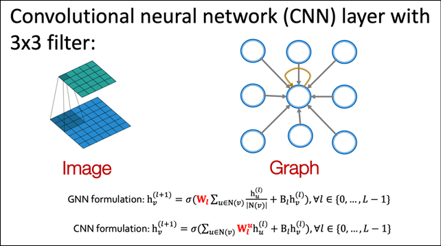
Figure 17.1: Parallels between convolutions in images and convolutions in graphs. Image source: CS-224W machine learning with Graphs, Stanford Univ.
The corresponding equations for the convolution operation on the CNN and the graph convolution are shown below. As you can see, on CNN, the convolution can be considered as a weighted linear combination of the input pixel and each of its neighbors. Each pixel brings its own weight in the form of the filter being applied. On the other hand, the graph convolution is also a weighted linear combination of the input pixel and an aggregate of all its neighbors. The aggregate effect of all neighbors is averaged into the convolution output:


Graph convolutions are thus a variation of convolutions that we are already familiar with. In the following section, we will see how these convolutions can be composed to build different kinds of GCN layers.
Common graph layers
All the graph layers that we discuss in this section use some variation of the graph convolution operation described above. Contributors to graph libraries such as DGL provide prebuilt versions of many of these layers within a short time of it being proposed in an academic paper, so you will realistically never have to implement one of these. The information here is mainly for understanding how things work under the hood.
Graph convolution network
The Graph Convolution Network (GCN) is the graph convolution layer proposed by Kipf and Welling [1]. It was originally presented as a scalable approach for semi-supervised learning on graph-structured data. They describe the GCN as an operation over the node feature vectors X and the adjacency matrix A of the underlying graph and point out that this can be exceptionally powerful when the information in A is not present in the data X, such as citation links between documents in a citation network, or relations in a knowledge graph.
GCNs combine the value of each node’s feature vector with those of its neighbors using some weights (initialized to random values). Thus, for every node, the sum of the neighboring node’s features is added. This operation can be represented as follows:

Here the update and aggregate are different kinds of summation functions. This sort of projection on node features is called a message-passing mechanism. A single iteration of this message passing is equivalent to a graph convolution over each node’s immediate neighbors. If we wish to incorporate information from more distant nodes, we can repeat this operation several times.
The following equation describes the output of the GCN at layer (l+1) at node i. Here, N(i) is the set of neighbors of node I (including itself), cij is the product of the square root of node degrees, and sigma is an activation function. The b(l) term is an optional bias term:

Next up, we will look at the graph attention network, a variant of the GCN where the coefficients are learned via an attentional mechanism instead of being explicitly defined.
Graph attention network
The Graph Attention Network (GAT) layer was proposed by Velickovic, et al. [2]. Like the GCN, the GAT performs local averaging of its neighbors’ features. The difference is instead of explicitly specifying the normalization term cij, the GAT allows it to be learned using self-attention over the node features to do so. The corresponding normalization term is written as ![]() for the GAT, which is computed based on the hidden features of the neighboring nodes and the learned attention vector. Essentially, the idea behind the GAT is to prioritize feature signals from similar neighbor nodes compared to dissimilar ones.
for the GAT, which is computed based on the hidden features of the neighboring nodes and the learned attention vector. Essentially, the idea behind the GAT is to prioritize feature signals from similar neighbor nodes compared to dissimilar ones.
Every neighbor ![]() neighborhood N(i) of node i sends its own vector of attentional coefficients
neighborhood N(i) of node i sends its own vector of attentional coefficients ![]() . The following set of equations describes the output of the GAT at layer (i+1) for node i. The attention
. The following set of equations describes the output of the GAT at layer (i+1) for node i. The attention ![]() is computed using Bahdanau’s attention model using a feedforward network:
is computed using Bahdanau’s attention model using a feedforward network:


GCN and GAT architectures are suitable for small to medium-sized networks. The GraphSAGE architecture, described in the next section, is more suitable for larger networks.
GraphSAGE (sample and aggregate)
So far, the convolutions we have considered require that all nodes in the graph be present during the training, and are therefore transductive and do not naturally generalize to unseen nodes. Hamilton, Ying, and Leskovec [3] proposed GraphSAGE, a general, inductive framework that can generate embeddings for previously unseen nodes. It does so by sampling and aggregating from a node’s local neighborhood. GraphSAGE has proved successful at node classification on temporally evolving networks such as citation graphs and Reddit post data.
GraphSAGE samples a subset of neighbors instead of using them all. It can define a node neighborhood using random walks and sum up importance scores to determine the optimum sample. An aggregate function can be one of MEAN, GCN, POOL, and LSTM. Mean aggregation simply takes the element-wise mean of the neighbor vectors. The LSTM aggregation is more expressive but is inherently sequential and not symmetric; it is applied on an unordered set derived from a random permutation of the node’s neighbors. The POOL aggregation is both symmetric and trainable; here, each neighbor vector is independently fed through a fully connected neural network and max pooling is applied across the aggregate information across the neighbor set.
This set of equations shows how the output for node i at layer (l+1) is generated from node i and its neighbors N(i) at layer l:


Now that we have seen strategies for handling large networks using GNNs, we will look at strategies for maximizing the representational (and therefore the discriminative) power of GNNs, using the graph isomorphism network.
Graph isomorphism network
Xu, et al. [4] proposed the Graph Isomorphism Network (GIN) as a graph layer with more expressive power compared to the ones available. Graph layers with high expressive power should be able to distinguish between a pair of graphs that are topologically similar but not identical. They showed that GCNs and GraphSAGE are unable to distinguish certain graph structures. They also showed that SUM aggregation is better than MEAN and MAX aggregation in terms of distinguishing graph structures. The GIN layer thus provides a better way to represent neighbor’s aggregation compared to GCNs and GraphSAGE.
The following equation shows the output at node i and layer (l+1). Here, the function fθ is a callable activation function, aggregate is an aggregation function such as SUM, MAX, or MEAN, and ![]() is a learnable parameter that will be learned over the course of the training:
is a learnable parameter that will be learned over the course of the training:

Having been introduced to several popular GNN architectures, let us now direct our attention to the kind of tasks we can do with GNNs.
Common graph applications
We will now look at some common applications of GNNs. Typically, applications fall into one of the three major classes listed below. In this section, we will see code examples on how to build and train GNNs for each of these tasks, using TensorFlow and DGL:
- Node classification
- Graph classification
- Edge classification (or link prediction)
There are other applications of GNNs as well, such as graph clustering or generative graph models, but they are less common and we will not consider them here.
Node classification
Node classification is a popular task on graph data. Here, a model is trained to predict the node category. Non-graph classification methods can use the node feature vectors alone to do so, and some pre-GNN methods such as DeepWalk and node2vec can use the adjacency matrix alone, but GNNs are the first class of techniques that can use both the node feature vectors and the connectivity information together to do node classification.
Essentially, the idea is to apply one or more graph convolutions (as described in the previous section) to all nodes of a graph, to project the feature vector of the node to a corresponding output category vector that can be used to predict the node category. Our node classification example will use the CORA dataset, a collection of 2,708 scientific papers classified into one of seven categories. The papers are organized into a citation network, which contains 5,429 links. Each paper is described by a word vector of size 1,433.
We first set up our imports. If you have not already done so, you will need to install the DGL library into your environment with pip install dgl. You will also need to set the environment variable DGLBACKEND to TensorFlow. On the command line, this is achieved by the command export DGLBACKEND=tensorflow, and in a notebook environment, you can try using the magic %env DGLBACKEND=tensorflow:
import dgl
import dgl.data
import matplotlib.pyplot as plt
import numpy as np
import os
import tensorflow as tf
import tensorflow_addons as tfa
from dgl.nn.tensorflow import GraphConv
The CORA dataset is pre-packaged as a DGL dataset, so we load the dataset into memory using the following call:
dataset = dgl.data.CoraGraphDataset()
The first time this is called, it will log that it is downloading and extracting to a local file. Once done, it will print out some useful statistics about the CORA dataset. As you can see, there are 2,708 nodes and 10,566 edges in the graph. Each node has a feature vector of size 1,433 and a node is categorized as being in one of seven classes. In addition, we see that it has 140 training samples, 500 validation samples, and 1,000 test samples:
  NumNodes: 2708
  NumEdges: 10556
  NumFeats: 1433
  NumClasses: 7
  NumTrainingSamples: 140
  NumValidationSamples: 500
  NumTestSamples: 1000
Done saving data into cached files.
Since this is a graph dataset, it is expected to contain data pertaining to a set of graphs. However, CORA is a single citation graph. You can verify this by len(dataset), which will give you 1. This also means that downstream code will work on the graph given by dataset[0] rather than on the complete dataset. The node features will be contained in the dictionary dataset[0].ndata as key-value pairs, and the edge features in dataset[0].edata. The ndata contains the keys train_mask, val_mask, and test_mask, which are Boolean masks signifying which nodes are part of the train, validation, and test splits, respectively, and a feat key, which contains the feature vector for each node in the graph.
We will build a NodeClassifier network with two GraphConv layers. Each layer will compute a new node representation by aggregating neighbor information. GraphConv layers are just simple tf.keras.layers.Layer objects and can therefore be stacked. The first GraphConv layer projects the incoming feature size (1,433) to a hidden feature vector of size 16, and the second GraphConv layer projects the hidden feature vector to an output category vector of size 2, from which the category is read.
Note that GraphConv is just one of many graph layers that we can drop into the NodeClassifier model. DGL makes available a variety of graph convolution layers that can be used to replace GraphConv if needed:
class NodeClassifier(tf.keras.Model):
  def __init__(self, g, in_feats, h_feats, num_classes):
    super(NodeClassifier, self).__init__()
    self.g = g
    self.conv1 = GraphConv(in_feats, h_feats, activation=tf.nn.relu)
    self.conv2 = GraphConv(h_feats, num_classes)
  def call(self, in_feat):
    h = self.conv1(self.g, in_feat)
    h = self.conv2(self.g, h)
    return h
g = dataset[0]
model = NodeClassifier(
  g, g.ndata["feat"].shape[1], 16, dataset.num_classes)
We will train this model with the CORA dataset using the code shown below. We will use the AdamW optimizer (a variation of the more popular Adam optimizer that results in models with better generalization capabilities), with a learning rate of 1e-2 and weight decay of 5e-4. We will train for 200 epochs. Let us also detect if we have a GPU available, and if so, assign the graph to the GPU.
TensorFlow will automatically move the model to the GPU if the GPU is detected:
def set_gpu_if_available():
  device = "/cpu:0"
  gpus = tf.config.list_physical_devices("GPU")
  if len(gpus) > 0:
    device = gpus[0]
  return device
device = set_gpu_if_available()
g = g.to(device)
We also define a do_eval() method that computes the accuracy given the features and the Boolean mask for the split being evaluated:
def do_eval(model, features, labels, mask):
  logits = model(features, training=False)
  logits = logits[mask]
  labels = labels[mask]
  preds = tf.math.argmax(logits, axis=1)
  acc = tf.reduce_mean(tf.cast(preds == labels, dtype=tf.float32))
  return acc.numpy().item()
Finally, we are ready to set up and run our training loop as follows:
NUM_HIDDEN = 16
LEARNING_RATE = 1e-2
WEIGHT_DECAY = 5e-4
NUM_EPOCHS = 200
with tf.device(device):
  feats = g.ndata["feat"]
  labels = g.ndata["label"]
  train_mask = g.ndata["train_mask"]
  val_mask = g.ndata["val_mask"]
  test_mask = g.ndata["test_mask"]
  in_feats = feats.shape[1]
  n_classes = dataset.num_classes
  n_edges = dataset[0].number_of_edges()
  model = NodeClassifier(g, in_feats, NUM_HIDDEN, n_classes)
  loss_fcn = tf.keras.losses.SparseCategoricalCrossentropy(from_logits=True)
  optimizer = tfa.optimizers.AdamW(
    learning_rate=LEARNING_RATE, weight_decay=WEIGHT_DECAY)
  best_val_acc, best_test_acc = 0, 0
  history = []
  for epoch in range(NUM_EPOCHS):
    with tf.GradientTape() as tape:
      logits = model(feats)
      loss = loss_fcn(labels[train_mask], logits[train_mask])
      grads = tape.gradient(loss, model.trainable_weights)
      optimizer.apply_gradients(zip(grads, model.trainable_weights))

    val_acc = do_eval(model, feats, labels, val_mask)
    history.append((epoch + 1, loss.numpy().item(), val_acc))
    if epoch % 10 == 0:
      print("Epoch {:3d} | train loss: {:.3f} | val acc: {:.3f}".format(
         epoch, loss.numpy().item(), val_acc))
The output of the training run shows the training loss decreasing from 1.9 to 0.02 and the validation accuracy increasing from 0.13 to 0.78:
Epoch   0 | train loss: 1.946 | val acc: 0.134
Epoch  10 | train loss: 1.836 | val acc: 0.544
Epoch  20 | train loss: 1.631 | val acc: 0.610
Epoch  30 | train loss: 1.348 | val acc: 0.688
Epoch  40 | train loss: 1.032 | val acc: 0.732
Epoch  50 | train loss: 0.738 | val acc: 0.760
Epoch  60 | train loss: 0.504 | val acc: 0.774
Epoch  70 | train loss: 0.340 | val acc: 0.776
Epoch  80 | train loss: 0.233 | val acc: 0.780
Epoch  90 | train loss: 0.164 | val acc: 0.780
Epoch 100 | train loss: 0.121 | val acc: 0.784
Epoch 110 | train loss: 0.092 | val acc: 0.784
Epoch 120 | train loss: 0.073 | val acc: 0.784
Epoch 130 | train loss: 0.059 | val acc: 0.784
Epoch 140 | train loss: 0.050 | val acc: 0.786
Epoch 150 | train loss: 0.042 | val acc: 0.786
Epoch 160 | train loss: 0.037 | val acc: 0.786
Epoch 170 | train loss: 0.032 | val acc: 0.784
Epoch 180 | train loss: 0.029 | val acc: 0.784
Epoch 190 | train loss: 0.026 | val acc: 0.784
We can now evaluate our trained node classifier against the hold-out test split:
test_acc = do_eval(model, feats, labels, test_mask)
print("Test acc: {:.3f}".format(test_acc))
This prints out the overall accuracy of the model against the hold-out test split:
Test acc: 0.779
Graph classification
Graph classification is done by predicting some attribute of the entire graph by aggregating all node features and applying one or more graph convolutions to it. This could be useful, for example, when trying to classify molecules during drug discovery as having a particular therapeutic property. In this section, we will showcase graph classification using an example.
In order to run the example, please make sure DGL is installed and set to use the TensorFlow backend; refer to the previous section on node classification for information on how to do this. To begin the example, let us import the necessary libraries:
import dgl.data
import tensorflow as tf
import tensorflow_addons as tfa
from dgl.nn import GraphConv
from sklearn.model_selection import train_test_split
We will use the protein dataset from DGL. The dataset is a set of graphs, each with node features and a single label. Each graph represents a protein molecule and each node in the graph represents an atom in the molecule. Node features list the chemical properties of the atom. The label indicates if the protein molecule is an enzyme:
dataset = dgl.data.GINDataset("PROTEINS", self_loop=True)
print("node feature dimensionality:", dataset.dim_nfeats)
print("number of graph categories:", dataset.gclasses)
print("number of graphs in dataset:", len(dataset))
The call above downloads the protein dataset locally and prints out some information about the dataset. As you can see, each node has a feature vector of size 3, the number of graph categories is 2 (enzyme or not), and the number of graphs in the dataset is 1113:
node feature dimensionality: 3
number of graph categories: 2
number of graphs in dataset: 1113
We will first split the dataset into training, validation, and test. We will use the training dataset to train our GNN, validate using the validation dataset, and publish the results of our final model against the test dataset:
tv_dataset, test_dataset = train_test_split(
  dataset, shuffle=True, test_size=0.2)
train_dataset, val_dataset = train_test_split(
  tv_dataset, test_size=0.1)
print(len(train_dataset), len(val_dataset), len(test_dataset))
This splits the dataset into a training, validation, and test split of 801, 89, and 223 graphs, respectively. Since our datasets are large, we need to train our network using mini-batches so as not to overwhelm GPU memory. So, this example will also demonstrate mini-batch processing using our data.
Next, we define our GNN for graph classification. This consists of two GraphConv layers stacked together that will encode the nodes into their hidden representations. Since the objective is to predict a single category for each graph, we need to aggregate all the node representations into a graph-level representation, which we do by averaging the node representations using dgl.mean_nodes():
class GraphClassifier(tf.keras.Model):
  def __init__(self, in_feats, h_feats, num_classes):
    super(GraphClassifier, self).__init__()
    self.conv1 = GraphConv(in_feats, h_feats, activation=tf.nn.relu)
    self.conv2 = GraphConv(h_feats, num_classes)
  def call(self, g, in_feat):
    h = self.conv1(g, in_feat)
    h = self.conv2(g, h)
    g.ndata["h"] = h
    return dgl.mean_nodes(g, "h")
For the training, we set the training parameters and the do_eval() function:
HIDDEN_SIZE = 16
BATCH_SIZE = 16
LEARNING_RATE = 1e-2
NUM_EPOCHS = 20
device = set_gpu_if_available()
def do_eval(model, dataset):
  total_acc, total_recs = 0, 0
  indexes = tf.data.Dataset.from_tensor_slices(range(len(dataset)))
  indexes = indexes.batch(batch_size=BATCH_SIZE)
  for batched_indexes in indexes:
    graphs, labels = zip(*[dataset[i] for i in batched_indexes])
    batched_graphs = dgl.batch(graphs)
    batched_labels = tf.convert_to_tensor(labels, dtype=tf.int64)
    batched_graphs = batched_graphs.to(device)
    logits = model(batched_graphs, batched_graphs.ndata["attr"])
    batched_preds = tf.math.argmax(logits, axis=1)
    acc = tf.reduce_sum(tf.cast(batched_preds == batched_labels,
                                dtype=tf.float32))
    total_acc += acc.numpy().item()
    total_recs += len(batched_labels)
  return total_acc / total_recs
Finally, we define and run our training loop to train our GraphClassifier model. We use the Adam optimizer with a learning rate of 1e-2 and the SparseCategoricalCrossentropy as the loss function, training, or 20 epochs:
with tf.device(device):
  model = GraphClassifier(
    dataset.dim_nfeats, HIDDEN_SIZE, dataset.gclasses)
  optimizer = tf.keras.optimizers.Adam(learning_rate=LEARNING_RATE)
  loss_fcn = tf.keras.losses.SparseCategoricalCrossentropy(
    from_logits=True)
  train_indexes = tf.data.Dataset.from_tensor_slices(
    range(len(train_dataset)))
  train_indexes = train_indexes.batch(batch_size=BATCH_SIZE)
  for epoch in range(NUM_EPOCHS):
    total_loss = 0
    for batched_indexes in train_indexes:
      with tf.GradientTape() as tape:
        graphs, labels = zip(*[train_dataset[i] for i in batched_indexes])
        batched_graphs = dgl.batch(graphs)
        batched_labels = tf.convert_to_tensor(labels, dtype=tf.int32)
        batched_graphs = batched_graphs.to(device)
        logits = model(batched_graphs, batched_graphs.ndata["attr"])
        loss = loss_fcn(batched_labels, logits)
        grads = tape.gradient(loss, model.trainable_weights)
        optimizer.apply_gradients(zip(grads, model.trainable_weights))
        total_loss += loss.numpy().item()

    val_acc = do_eval(model, val_dataset)
    print("Epoch {:3d} | train_loss: {:.3f} | val_acc: {:.3f}".format(
        epoch, total_loss, val_acc))
The output shows that the loss decreases and validation accuracy increases as the GraphClassifier model is trained over 20 epochs:
Epoch   0 | train_loss: 34.401 | val_acc: 0.629
Epoch   1 | train_loss: 33.868 | val_acc: 0.629
Epoch   2 | train_loss: 33.554 | val_acc: 0.618
Epoch   3 | train_loss: 33.184 | val_acc: 0.640
Epoch   4 | train_loss: 32.822 | val_acc: 0.652
Epoch   5 | train_loss: 32.499 | val_acc: 0.663
Epoch   6 | train_loss: 32.227 | val_acc: 0.663
Epoch   7 | train_loss: 32.009 | val_acc: 0.697
Epoch   8 | train_loss: 31.830 | val_acc: 0.685
Epoch   9 | train_loss: 31.675 | val_acc: 0.685
Epoch  10 | train_loss: 31.580 | val_acc: 0.685
Epoch  11 | train_loss: 31.525 | val_acc: 0.708
Epoch  12 | train_loss: 31.485 | val_acc: 0.708
Epoch  13 | train_loss: 31.464 | val_acc: 0.708
Epoch  14 | train_loss: 31.449 | val_acc: 0.708
Epoch  15 | train_loss: 31.431 | val_acc: 0.708
Epoch  16 | train_loss: 31.421 | val_acc: 0.708
Epoch  17 | train_loss: 31.411 | val_acc: 0.708
Epoch  18 | train_loss: 31.404 | val_acc: 0.719
Epoch  19 | train_loss: 31.398 | val_acc: 0.719
Finally, we evaluate the trained model against our hold-out test dataset:
test_acc = do_eval(model, test_dataset)
print("test accuracy: {:.3f}".format(test_acc))
This prints out the accuracy of the trained GraphClassifier model against the held-out test split:
test accuracy: 0.677
The accuracy shows that the model can successfully identify a molecule as an enzyme or non-enzyme slightly less than 70% of the time.
Link prediction
Link prediction is a type of edge classification problem, where the task is to predict if an edge exists between two given nodes in the graph.
Many applications, such as social recommendation, knowledge graph completion, etc., can be formulated as link prediction, which predicts whether an edge exists between a pair of nodes. In this example, we will predict if a citation relationship, either citing or cited, exists between two papers in a citation network.
The general approach would be to treat all edges in the graph as positive examples and sample a number of non-existent edges as negative examples and train the link prediction classifier for binary classification (edge exists or not) on these positive and negative examples.
Before running the example, please make sure DGL is installed and set to use the TensorFlow backend; refer to the Node classification section for information on how to do this. Let us start by importing the necessary libraries:
import dgl
import dgl.data
import dgl.function as fn
import tensorflow as tf
import itertools
import numpy as np
import scipy.sparse as sp
from dgl.nn import SAGEConv
from sklearn.metrics import roc_auc_score
For our data, we will reuse the CORA citation graph from the DGL datasets that we had used for our node classification example earlier. We already know what the dataset looks like, so we won’t dissect it again here. If you would like to refresh your memory, please refer to the node classification example for the relevant details:
dataset = dgl.data.CoraGraphDataset()
g = dataset[0]
Now, let us prepare our data. For training our link prediction model, we need a set of positive edges and a set of negative edges. Positive edges are one of the 10,556 edges that already exist in the CORA citation graph, and negative edges are going to be 10,556 node pairs without connecting edges sampled from the rest of the graph. In addition, we need to split both the positive and negative edges into training, validation, and test splits:
u, v = g.edges()
# positive edges
eids = np.arange(g.number_of_edges())
eids = np.random.permutation(eids)
test_size = int(len(eids) * 0.2)
val_size = int((len(eids) - test_size) * 0.1)
train_size = g.number_of_edges() - test_size - val_size
u = u.numpy()
v = v.numpy()
test_pos_u = u[eids[0:test_size]]
test_pos_v = v[eids[0:test_size]]
val_pos_u = u[eids[test_size:test_size + val_size]]
val_pos_v = v[eids[test_size:test_size + val_size]]
train_pos_u = u[eids[test_size + val_size:]]
train_pos_v = v[eids[test_size + val_size:]]
# negative edges
adj = sp.coo_matrix((np.ones(len(u)), (u, v)))
adj_neg = 1 - adj.todense() - np.eye(g.number_of_nodes())
neg_u, neg_v = np.where(adj_neg != 0)
neg_eids = np.random.choice(len(neg_u), g.number_of_edges())
test_neg_u = neg_u[neg_eids[:test_size]]
test_neg_v = neg_v[neg_eids[:test_size]]
val_neg_u = neg_u[neg_eids[test_size:test_size + val_size]]
val_neg_v = neg_v[neg_eids[test_size:test_size + val_size]]
train_neg_u = neg_u[neg_eids[test_size + val_size:]]
train_neg_v = neg_v[neg_eids[test_size + val_size:]]
# remove edges from training graph
test_edges = eids[:test_size]
val_edges = eids[test_size:test_size + val_size]
train_edges = eids[test_size + val_size:]
train_g = dgl.remove_edges(g, np.concatenate([test_edges, val_edges]))
We now construct a GNN that will compute the node representation using two GraphSAGE layers, each layer computing the node representation by averaging its neighbor information:
class LinkPredictor(tf.keras.Model):
  def __init__(self, g, in_feats, h_feats):
    super(LinkPredictor, self).__init__()
    self.g = g
    self.conv1 = SAGEConv(in_feats, h_feats, 'mean')
    self.relu1 = tf.keras.layers.Activation(tf.nn.relu)
    self.conv2 = SAGEConv(h_feats, h_feats, 'mean')
  def call(self, in_feat):
    h = self.conv1(self.g, in_feat)
    h = self.relu1(h)
    h = self.conv2(self.g, h)
    return h
However, link prediction requires us to compute representations of pairs of nodes, DGL recommends that you treat the pairs of nodes as another graph since you can define a pair of nodes as an edge. For link prediction, we will have a positive graph containing all the positive examples as edges, and a negative graph containing all the negative examples as edges. Both positive and negative graphs contain the same set of nodes as the original graph:
train_pos_g = dgl.graph((train_pos_u, train_pos_v),
  num_nodes=g.number_of_nodes())
train_neg_g = dgl.graph((train_neg_u, train_neg_v),
  num_nodes=g.number_of_nodes())
val_pos_g = dgl.graph((val_pos_u, val_pos_v),
  num_nodes=g.number_of_nodes())
val_neg_g = dgl.graph((val_neg_u, val_neg_v),
  num_nodes=g.number_of_nodes())
test_pos_g = dgl.graph((test_pos_u, test_pos_v),
  num_nodes=g.number_of_nodes())
test_neg_g = dgl.graph((test_neg_u, test_neg_v),
  num_nodes=g.number_of_nodes())
Next, we will define a predictor class that will take the set of node representations from the LinkPredictor class and use the DGLGraph.apply_edges method to compute edge feature scores, which are the dot product of the source node features and the destination node features (both output together from the LinkPredictor in this case):
class DotProductPredictor(tf.keras.Model):
  def call(self, g, h):
    with g.local_scope():
      g.ndata['h'] = h
      # Compute a new edge feature named 'score' by a dot-product
      # between the source node feature 'h' and destination node
      # feature 'h'.
      g.apply_edges(fn.u_dot_v('h', 'h', 'score'))
      # u_dot_v returns a 1-element vector for each edge so you
      # need to squeeze it.
      return g.edata['score'][:, 0]
You can also build a custom predictor such as a multi-layer perceptron with two dense layers, as the following code shows. Note that the apply_edges method describes how the edge score is calculated:
class MLPPredictor(tf.keras.Model):
  def __init__(self, h_feats):
    super().__init__()
    self.W1 = tf.keras.layers.Dense(h_feats, activation=tf.nn.relu)
    self.W2 = tf.keras.layers.Dense(1)
  def apply_edges(self, edges):
    h = tf.concat([edges.src["h"], edges.dst["h"]], axis=1)
    return {
      "score": self.W2(self.W1(h))[:, 0]
    }
  def call(self, g, h):
    with g.local_scope():
      g.ndata['h'] = h
      g.apply_edges(self.apply_edges)
      return g.edata['score']
We instantiate the LinkPredictor model we defined earlier, select the Adam optimizer, and declare our loss function to be BinaryCrossEntropy (since our task is binary classification). The predictor head that we will use in our example is the DotProductPredictor. However, the MLPPredictor can be used as a drop-in replacement instead; just replace the pred variable below to point to the MLPPredictor instead of the DotProductPredictor:
HIDDEN_SIZE = 16
LEARNING_RATE = 1e-2
NUM_EPOCHS = 100
model = LinkPredictor(train_g, train_g.ndata['feat'].shape[1],
    HIDDEN_SIZE)
optimizer = tf.keras.optimizers.Adam(learning_rate=LEARNING_RATE)
loss_fcn = tf.keras.losses.BinaryCrossentropy(from_logits=True)
pred = DotProductPredictor()
We also define a couple of convenience functions for our training loop. The first one computes the loss between the scores returned from the positive graph and the negative graphs, and the second computes the Area Under the Curve (AUC) from the two scores. AUC is a popular metric to evaluate binary classification models:
def compute_loss(pos_score, neg_score):
    scores = tf.concat([pos_score, neg_score], axis=0)
    labels = tf.concat([
      tf.ones(pos_score.shape[0]),
      tf.zeros(neg_score.shape[0])
    ], axis=0
)
    return loss_fcn(labels, scores)
def compute_auc(pos_score, neg_score):
    scores = tf.concat([pos_score, neg_score], axis=0).numpy()
    labels = tf.concat([
      tf.ones(pos_score.shape[0]),
      tf.zeros(neg_score.shape[0])
    ], axis=0).numpy()
    return roc_auc_score(labels, scores)
We now train our LinkPredictor GNN for 100 epochs of training, using the following training loop:
for epoch in range(NUM_EPOCHS):
  in_feat = train_g.ndata["feat"]
  with tf.GradientTape() as tape:
    h = model(in_feat)
    pos_score = pred(train_pos_g, h)
    neg_score = pred(train_neg_g, h)
    loss = compute_loss(pos_score, neg_score)
    grads = tape.gradient(loss, model.trainable_weights)
    optimizer.apply_gradients(zip(grads, model.trainable_weights))
  val_pos_score = pred(val_pos_g, h)
  val_neg_score = pred(val_neg_g, h)
  val_auc = compute_auc(val_pos_score, val_neg_score)
  if epoch % 5 == 0:
    print("Epoch {:3d} | train_loss: {:.3f}, val_auc: {:.3f}".format(
      epoch, loss, val_auc))
This returns the following training logs:
Epoch   0 | train_loss: 0.693, val_auc: 0.566
Epoch   5 | train_loss: 0.681, val_auc: 0.633
Epoch  10 | train_loss: 0.626, val_auc: 0.746
Epoch  15 | train_loss: 0.569, val_auc: 0.776
Epoch  20 | train_loss: 0.532, val_auc: 0.805
Epoch  25 | train_loss: 0.509, val_auc: 0.820
Epoch  30 | train_loss: 0.492, val_auc: 0.824
Epoch  35 | train_loss: 0.470, val_auc: 0.833
Epoch  40 | train_loss: 0.453, val_auc: 0.835
Epoch  45 | train_loss: 0.431, val_auc: 0.842
Epoch  50 | train_loss: 0.410, val_auc: 0.851
Epoch  55 | train_loss: 0.391, val_auc: 0.859
Epoch  60 | train_loss: 0.371, val_auc: 0.861
Epoch  65 | train_loss: 0.350, val_auc: 0.861
Epoch  70 | train_loss: 0.330, val_auc: 0.861
Epoch  75 | train_loss: 0.310, val_auc: 0.862
Epoch  80 | train_loss: 0.290, val_auc: 0.860
Epoch  85 | train_loss: 0.269, val_auc: 0.856
Epoch  90 | train_loss: 0.249, val_auc: 0.852
Epoch  95 | train_loss: 0.228, val_auc: 0.848
We can now evaluate the trained model against the hold-out test set:
pos_score = tf.stop_gradient(pred(test_pos_g, h))
neg_score = tf.stop_gradient(pred(test_neg_g, h))
print('Test AUC', compute_auc(pos_score, neg_score))
This returns the following test AUC for our LinkPredictor GNN:
Test AUC 0.8266960571287392
This is quite impressive as it implies that the link predictor can correctly predict 82% of the links presented as ground truths in the test set.
Graph customizations
We have seen how to build and train GNNs for common graph ML tasks. However, for convenience, we have chosen to use prebuilt DGL graph convolution layers in our models. While unlikely, it is possible that you might need a layer that is not provided with the DGL package. DGL provides a message passing API to allow you to build custom graph layers easily. In the first part of this section, we will look at an example where we use the message-passing API to build a custom graph convolution layer.
We have also loaded datasets from the DGL data package for our examples. It is far more likely that we will need to use our own data instead. So, in the second part of this section, we will see how to convert our own data into a DGL dataset.
Custom layers and message passing
Although DGL provides many graph layers out of the box, there may be cases where the ones provided don’t meet our needs exactly and we need to build your own.
Fortunately, all these graph layers are based on a common underlying concept of message passing between nodes in the graph. So, in order to build a custom GNN layer, you need to understand how the message-passing paradigm works. This paradigm is also known as the Message Passing Neural Network (MPNN) framework [5]:


Each node u in the graph has a hidden state (initially its feature vector) represented by hu. For each node u and v, where nodes u and v are neighbors, i.e., connected by an edge eu->v, we apply some function M called the message function. The message function M is applied to every node on the graph. We then aggregate the output of M for all nodes with the output of all their neighboring nodes to produce the message m. Here ![]() is called the reduce function. Note that even though we represent the reduce function by the summation symbol
is called the reduce function. Note that even though we represent the reduce function by the summation symbol ![]() , it can be any aggregation function. Finally, we update the hidden state of node v using the obtained message and the previous state of the node. The function U applied at this step is called the update function.
, it can be any aggregation function. Finally, we update the hidden state of node v using the obtained message and the previous state of the node. The function U applied at this step is called the update function.
The message-passing algorithm is repeated a specific number of times. After that, we reach the readout phase where we extract the feature vector from each node that represents the entire graph. For example, the final feature vector for a node might represent the node category in the case of node classification.
In this section, we will use the MPNN framework to implement a GraphSAGE layer. Even though DGL provides the dgl.nn.SAGEConv, which implements this already, this is an example to illustrate the creation of custom graph layers using MPNN. The message-passing steps of a GraphSAGE layer are given by:


The code to implement our custom GraphSAGE layer using MPNN is shown below. The DGL function update_all call allows you to specify a message_fn and a reduce_fn, which are also DGL built-in functions, and the tf.concat and Dense layers represent the final update function:
import dgl
import dgl.data
import dgl.function as fn
import tensorflow as tf
class CustomGraphSAGE(tf.keras.layers.Layer):
  def __init__(self, in_feat, out_feat):
    super(CustomGraphSAGE, self).__init__()
    # A linear submodule for projecting the input and neighbor
    # feature to the output.
    self.linear = tf.keras.layers.Dense(out_feat, activation=tf.nn.relu)
  def call(self, g, h):
    with g.local_scope():
        g.ndata["h"] = h
        # update_all is a message passing API.
        g.update_all(message_func=fn.copy_u('h', 'm'),
                     reduce_func=fn.mean('m', 'h_N'))
        h_N = g.ndata['h_N']
        h_total = tf.concat([h, h_N], axis=1)
        return self.linear(h_total)
Here, we see that the update_all function specifies a message_func, which just copies the node’s current feature vector to a message vector m, and then averages all the message vectors in the neighborhood of each node. As you can see, this faithfully follows the first GraphSAGE equation above. DGL provides many such built-in functions (https://docs.dgl.ai/api/python/dgl.function.html).
Once the neighborhood vector h_N is computed in the first step, it is concatenated with the input feature vector h, and then passed through a Dense layer with a ReLU activation, as described by the second equation for GraphSAGE above. We have thus implemented the GraphSAGE layer with our CustomGraphSAGE object.
The next step is to put it into a GNN to see how it works. The following code shows a CustomGNN model that uses two layers of our custom SAGEConv implementation:
class CustomGNN(tf.keras.Model):
  def __init__(self, g, in_feats, h_feats, num_classes):
    super(CustomGNN, self).__init__()
    self.g = g
    self.conv1 = CustomGraphSAGE(in_feats, h_feats)
    self.relu1 = tf.keras.layers.Activation(tf.nn.relu)
    self.conv2 = CustomGraphSAGE(h_feats, num_classes)
  def call(self, in_feat):
    h = self.conv1(self.g, in_feat)
    h = self.relu1(h)
    h = self.conv2(self.g, h)
    return h
We will run it to do node classification against the CORA dataset, details of which should be familiar from previous examples.
The above code assumes an unweighted graph, i.e., edges between nodes have the same weight. This condition is true for the CORA dataset, where each edge represents a citation from one paper to another.
However, we can imagine scenarios where edges may be weighted based on how many times some edge has been invoked, for example, an edge that connects a product and a user for user recommendations.
The only change we need to make to handle weighted edges is to allow the weight to play a part in our message function. That is, if an edge between our node u and a neighbor node v occurs k times, we should consider that edge k times. The code below shows our custom GraphSAGE layer with the ability to handle weighted edges:
class CustomWeightedGraphSAGE(tf.keras.layers.Layer):
  def __init__(self, in_feat, out_feat):
    super(CustomWeightedGraphSAGE, self).__init__()
    # A linear submodule for projecting the input and neighbor
    # feature to the output.
    self.linear = tf.keras.layers.Dense(out_feat, activation=tf.nn.relu)
  def call(self, g, h, w):
    with g.local_scope():
      g.ndata['h'] = h
      g.edata['w'] = w
      g.update_all(message_func=fn.u_mul_e('h', 'w', 'm'),
                   reduce_func=fn.mean('m', 'h_N'))
      h_N = g.ndata['h_N']
      h_total = tf.concat([h, h_N], axis=1)
      return self.linear(h_total)
This code expects an additional edge property w, which contains the edge weights, which you can simulate on the CORA dataset by:
g.edata["w"] = tf.cast(
   tf.random.uniform((g.num_edges(), 1), minval=3, maxval=10,
                     dtype=tf.int32),
   dtype=tf.float32)
The message_func in CustomWeightedGraphSAGE has changed from simply copying the feature vector h to the message vector m, to multiplying h and w to produce the message vector m. Everything else is the same as in CustomGraphSAGE. The new CustomWeightedGraphSAGE layer can now be simply dropped into the calling class CustomGNN where CustomGraphSAGE was originally being called.
Custom graph dataset
A more common use case that you are likely to face is to use your own data to train a GNN model. Obviously, in such cases, you cannot use a DGL-provided dataset (as we have been using in all our examples so far) and you must wrap your data into a custom graph dataset.
Your custom graph dataset should inherit from the dgl.data.DGLDataset object provided by DGL and implement the following methods:
__getitem__(self, i)– retrieve thei-th example from the dataset. The retrieved example contains a single DGL graph and its label if applicable.__len__(self)– the number of examples in the dataset.process(self)– defines how to load and process raw data from the disk.
As we have seen before, node classification and link prediction operate on a single graph, and graph classification operates on a set of graphs. While the approach is largely identical for both cases, there are some concerns specific to either case, so we will provide an example to do each of these below.
Single graphs in datasets
For our example, we will choose Zachary’s Karate Club graph, which represents the members of a Karate Club observed over three years. Over time, there was a disagreement between an administrator (Officer) and the instructor (Mr. Hi), and the club members split and reformed under the Officer and Mr. Hi (shown below as blue and red nodes, respectively). The Zachary Karate Club network is available for download from the NetworkX library:
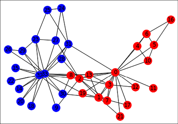
Figure 17.2: Graph representation of the Karate Club Network
The graph contains 34 nodes labeled with one of “Officer” or “Mr. Hi” depending on which group they ended up in after the split. It contains 78 edges, which are undirected and unweighted. An edge between a pair of members indicates that they interact with each other outside the club. To make this dataset more realistic for GNN usage, we will attach a 10-dimensional random feature vector to each node, and an edge weight as an edge feature. Here is the code to convert the Karate Club graph into a DGL dataset that you can then use for downstream node or edge classification tasks:
class KarateClubDataset(DGLDataset):
  def __init__(self):
    super().__init__(name="karate_club")
  def __getitem__(self, i):
    return self.graph
  def __len__(self):
    return 1
  def process(self):
    G = nx.karate_club_graph()
    nodes = [node for node in G.nodes]
    edges = [edge for edge in G.edges]
    node_features = tf.random.uniform(
        (len(nodes), 10), minval=0, maxval=1, dtype=tf.dtypes.float32)
    label2int = {"Mr. Hi": 0, "Officer": 1}
    node_labels = tf.convert_to_tensor(
        [label2int[G.nodes[node]["club"]] for node in nodes])
    edge_features = tf.random.uniform(
        (len(edges), 1), minval=3, maxval=10, dtype=tf.dtypes.int32)
    edges_src = tf.convert_to_tensor([u for u, v in edges])
    edges_dst = tf.convert_to_tensor([v for u, v in edges])
    self.graph = dgl.graph((edges_src, edges_dst), num_nodes=len(nodes))
    self.graph.ndata["feat"] = node_features
    self.graph.ndata["label"] = node_labels
    self.graph.edata["weight"] = edge_features
    # assign masks indicating the split (training, validation, test)
    n_nodes = len(nodes)
    n_train = int(n_nodes * 0.6)
    n_val = int(n_nodes * 0.2)
    train_mask = tf.convert_to_tensor(
      np.hstack([np.ones(n_train), np.zeros(n_nodes - n_train)]),
      dtype=tf.bool)
    val_mask = tf.convert_to_tensor(
      np.hstack([np.zeros(n_train), np.ones(n_val),
                 np.zeros(n_nodes - n_train - n_val)]),
      dtype=tf.bool)
    test_mask = tf.convert_to_tensor(
      np.hstack([np.zeros(n_train + n_val),
                 np.ones(n_nodes - n_train - n_val)]),
      dtype=tf.bool)
    self.graph.ndata["train_mask"] = train_mask
    self.graph.ndata["val_mask"] = val_mask
    self.graph.ndata["test_mask"] = test_mask
Most of the logic is in the process method. We call the NetworkX method to get the Karate Club as a NetworkX graph, then convert it to a DGL graph object with node features and labels. Even though the Karate Club graph does not have node and edge features defined, we manufacture some random numbers and set them to these properties. Note that this is only for purposes of this example, to show where these features would need to be updated if your graph had node and edge features. Note that the dataset contains a single graph.
In addition, we also want to split the graph into training, validation, and test splits for node classification purposes. For that, we assign masks indicating whether a node belongs to one of these splits. We do this rather simply by splitting the nodes in the graph 60/20/20 and assigning Boolean masks for each split.
In order to instantiate this dataset from our code, we can say:
dataset = KarateClubDataset()
g = dataset[0]
print(g)
This will give us the following output (reformatted a little for readability). The two main structures are the ndata_schemas and edata_schemas, accessible as g.ndata and g.edata, respectively. Within ndata_schemas, we have keys that point to the node features (feats), node labels (label), and the masks to indicate the training, validation, and test splits (train_mask, val_mask, and test_mask), respectively. Under edata_schemas, there is the weight attribute that indicates the edge weights:
Graph(num_nodes=34,
      num_edges=78,
      ndata_schemes={
        'feat': Scheme(shape=(10,), dtype=tf.float32),
        'label': Scheme(shape=(), dtype=tf.int32),
        'train_mask': Scheme(shape=(), dtype=tf.bool),
        'val_mask': Scheme(shape=(), dtype=tf.bool),
        'test_mask': Scheme(shape=(), dtype=tf.bool)
      }
      edata_schemes={
         'weight': Scheme(shape=(1,), dtype=tf.int32)
      }
)
Please refer to the examples on node classification and link prediction for information on how to use this kind of custom dataset.
Set of multiple graphs in datasets
Datasets that support the graph classification task will contain multiple graphs and their associated labels, one per graph. For our example, we will consider a hypothetical dataset of molecules represented as graphs, and the task would be to predict if the molecule is toxic or not (a binary prediction).
We will use the NetworkX method random_regular_graph() to generate synthetic graphs with a random number of nodes and node degree. To each node of each graph, we will attach a random 10-dimensional feature vector. Each node will have a label (0 or 1) indicating if the graph is toxic. Note that this is just a simulation of what real data might look like. With real data, the structure of each graph and the values of the node vectors, which are random in our case, will have a real impact on the target variable, i.e., the toxicity of the molecule.
The figure below shows some examples of what the synthetic “molecules” might look like:
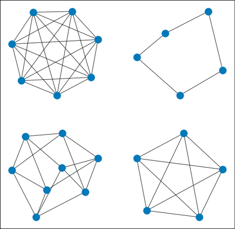
Figure 17.3: Some examples of random regular graphs generated using NetworkX
Here is the code to convert a set of random NetworkX graphs into a DGL graph dataset for graph classification. We will generate 100 such graphs and store them in a list in the form of a DGL dataset:
from networkx.exception import NetworkXError
class SyntheticDataset(DGLDataset):
  def __init__(self):
    super().__init__(name="synthetic")
  def __getitem__(self, i):
    return self.graphs[i], self.labels[i]
  def __len__(self):
    return len(self.graphs)
  def process(self):
    self.graphs, self.labels = [], []
    num_graphs = 0
    while(True):
      d = np.random.randint(3, 10)
      n = np.random.randint(5, 10)
      if ((n * d) % 2) != 0:
        continue
      if n < d:
        continue
      try:
        g = nx.random_regular_graph(d, n)
      except NetworkXError:
        continue
      g_edges = [edge for edge in g.edges]
      g_src = [u for u, v in g_edges]
      g_dst = [v for u, v in g_edges]
      g_num_nodes = len(g.nodes)
      label = np.random.randint(0, 2)
      # create graph and add to list of graphs and labels
      dgl_graph = dgl.graph((g_src, g_dst), num_nodes=g_num_nodes)
      dgl_graph.ndata["feats"] = tf.random.uniform(
          (g_num_nodes, 10), minval=0, maxval=1, dtype=tf.dtypes.float32)
      self.graphs.append(dgl_graph)
      self.labels.append(label)
      num_graphs += 1
      if num_graphs > 100:
        break
    self.labels = tf.convert_to_tensor(self.labels, dtype=tf.dtypes.int64)
Once created, we can then call it from our code as follows:
dataset = SyntheticDataset()
graph, label = dataset[0]
print(graph)
print("label:", label)
This produces the following output for the first graph in the DGL dataset (reformatted slightly for readability). As you can see, the first graph in the dataset has 6 nodes and 15 edges and contains a feature vector (accessible using the feats key) of size 10. The label is a 0-dimensional tensor (i.e., a scalar) of type long (int64):
Graph(num_nodes=6, num_edges=15,
      ndata_schemes={
        'feats': Scheme(shape=(10,), dtype=tf.float32)}
      edata_schemes={})
label: tf.Tensor(0, shape=(), dtype=int64)
As before, in order to see how you would use this custom dataset for some task such as graph classification, please refer to the example on graph classification earlier in this chapter.
Future directions
Graph neural networks are a rapidly evolving discipline. We have covered working with static homogeneous graphs on various popular graph tasks so far, which covers many real-world use cases. However, it is likely that some graphs are neither homogeneous nor static, and neither can they be easily reduced to this form. In this section, we will look at our options for dealing with heterogenous and temporal graphs.
Heterogeneous graphs
Heterogeneous graphs [7], also called heterographs, differ from the graphs we have seen so far in that they may contain different kinds of nodes and edges. These different types of nodes and edges might also contain different types of attributes, including possible representations with different dimensions. Popular examples of heterogeneous graphs are citation graphs that contain authors and papers, recommendation graphs that contain users and products, and knowledge graphs that can contain many different types of entities.
You can use the MPNN framework on heterogeneous graphs by manually implementing message and update functions individually for each edge type. Each edge type is defined by the triple (source node type, edge type, and destination node type). However, DGL provides support for heterogeneous graphs using the dgl.heterograph() API, where a graph is specified as a series of graphs, one per edge type.
Typical learning tasks associated with heterogeneous graphs are similar to their homogeneous counterparts, namely node classification and regression, graph classification, and edge classification/link prediction. A popular graph layer for working with heterogeneous graphs is the Relational GCN or R-GCN, available as a built-in layer in DGL.
Temporal Graphs
Temporal Graphs [8] is a framework developed at Twitter to handle dynamic graphs that change over time. While GNN models have primarily focused on static graphs that do not change over time, adding the time dimension allows us to model many interesting phenomena in social networks, financial transactions, and recommender systems, all of which are inherently dynamic. In such systems, it is the dynamic behavior that conveys the important insights.
A dynamic graph can be represented as a stream of timed events, such as additions and deletions of nodes and edges. This stream of events is fed into an encoder network that learns a time-dependent encoding for each node in the graph. A decoder is trained on this encoding to support some specific task such as link prediction at a future point in time. There is currently no support in the DGL library for Temporal Graphs, mainly because it is a very rapidly evolving research area.
At a high level, a Temporal Graph Network (TGN) encoder works by creating a compressed representation of the nodes based on their interaction and updates over time. The current state of each node is stored in TGN memory and acts as the hidden state st of an RNN; however, we have a separate state vector st(t) for each node i and time point t.
A message function similar to what we have seen in the MPNN framework computes two messages mi and mj for a pair of nodes i and j using the state vectors and their interaction as input. The message and state vectors are then combined using a memory updater, which is usually implemented as an RNN. TGNs have been found to outperform their static counterparts on the tasks of future edge prediction and dynamic node classification both in terms of accuracy and speed.
Summary
In this chapter, we have covered graph neural networks, an exciting set of techniques to learn not only from node features but also from the interaction between nodes. We have covered the intuition behind why graph convolutions work and the parallels between them and convolutions in computer vision. We have described some common graph convolutions, which are provided as layers by DGL. We have demonstrated how to use the DGL for popular graph tasks of node classification, graph classification, and link prediction. In addition, in the unlikely event that our needs are not met by standard DGL graph layers, we have learned how to implement our own graph convolution layer using DGL’s message-passing framework. We have also seen how to build DGL datasets for our own graph data. Finally, we look at some emerging directions of graph neural networks, namely heterogeneous graphs and temporal graphs. This should equip you with skills to use GNNs to solve interesting problems in this area.
In the next chapter, we will turn our attention to learning about some best ML practices associated with deep learning projects.
References
- Kipf, T. and Welling, M. (2017). Semi-supervised Classification with Graph Convolutional Networks. Arxiv Preprint, arXiv: 1609.02907 [cs.LG]. Retrieved from https://arxiv.org/abs/1609.02907
- Velickovic, P., et al. (2018). Graph Attention Networks. Arxiv Preprint, arXiv 1710.10903 [stat.ML]. Retrieved from https://arxiv.org/abs/1710.10903
- Hamilton, W. L., Ying, R., and Leskovec, J. (2017). Inductive Representation Learning on Large Graphs. Arxiv Preprint, arXiv: 1706.02216 [cs.SI]. Retrieved from https://arxiv.org/abs/1706.02216
- Xu, K., et al. (2018). How Powerful are Graph Neural Networks?. Arxiv Preprint, arXiv: 1810.00826 [cs.LG]. Retrieved from https://arxiv.org/abs/1810.00826
- Gilmer, J., et al. (2017). Neural Message Passing for Quantum Chemistry. Arxiv Preprint, arXiv: 1704.01212 [cs.LG]. Retrieved from https://arxiv.org/abs/1704.01212
- Zachary, W. W. (1977). An Information Flow Model for Conflict and Fission in Small Groups. Journal of Anthropological Research. Retrieved from https://www.journals.uchicago.edu/doi/abs/10.1086/jar.33.4.3629752
- Pengfei, W. (2020). Working with Heterogeneous Graphs in DGL. Blog post. Retrieved from https://www.jianshu.com/p/767950b560c4
- Bronstein, M. (2020). Temporal Graph Networks. Blog post. Retrieved from https://towardsdatascience.com/temporal-graph-networks-ab8f327f2efe
Join our book’s Discord space
Join our Discord community to meet like-minded people and learn alongside more than 2000 members at: https://packt.link/keras
