
20
Advanced Convolutional Neural Networks
In this chapter, we will see some more advanced uses for Convolutional Neural Networks (CNNs). We will explore:
- How CNNs can be applied within the areas of computer vision, video, textual documents, audio, and music
- How to use CNNs for text processing
- What capsule networks are
- Computer vision
All the code files for this chapter can be found at https://packt.link/dltfchp20.
Let’s start by using CNNs for complex tasks.
Composing CNNs for complex tasks
We have discussed CNNs quite extensively in Chapter 3, Convolutional Neural Networks, and at this point, you are probably convinced about the effectiveness of the CNN architecture for image classification tasks. What you may find surprising, however, is that the basic CNN architecture can be composed and extended in various ways to solve a variety of more complex tasks. In this section, we will look at the computer vision tasks mentioned in Figure 20.1 and show how they can be solved by turning CNNs into larger and more complex architectures.

Figure 20.1: Different Computer Vision Tasks – source: Introduction to Artificial Intelligence and Computer Vision Revolution (https://www.slideshare.net/darian_f/introduction-to-the-artificial-intelligence-and-computer-vision-revolution)
Classification and localization
In the classification and localization task, not only do you have to report the class of object found in the image, but also the coordinates of the bounding box where the object appears in the image. This type of task assumes that there is only one instance of the object in an image.
This can be achieved by attaching a “regression head” in addition to the “classification head” in a typical classification network. Recall that in a classification network, the final output of convolution and pooling operations, called the feature map, is fed into a fully connected network that produces a vector of class probabilities. This fully connected network is called the classification head, and it is tuned using a categorical loss function (Lc) such as categorical cross-entropy.
Similarly, a regression head is another fully connected network that takes the feature map and produces a vector (x, y, w, h) representing the top left x and y coordinates, and the width and height of the bounding box. It is tuned using a continuous loss function (LR) such as mean squared error. The entire network is tuned using a linear combination of the two losses, i.e.,

Here, ![]() is a hyperparameter and can take a value between 0 and 1. Unless the value is determined by some domain knowledge about the problem, it can be set to 0.5.
is a hyperparameter and can take a value between 0 and 1. Unless the value is determined by some domain knowledge about the problem, it can be set to 0.5.
Figure 20.2 shows a typical classification and localization network architecture:

Figure 20.2: Network architecture for image classification and localization
As you can see, the only difference with respect to a typical CNN classification network is the additional regression head at the top right-hand side.
Semantic segmentation
Another class of problem that builds on the basic classification idea is “semantic segmentation.” Here the aim is to classify every single pixel on the image as belonging to a single class.
An initial method of implementation could be to build a classifier network for each pixel, where the input is a small neighborhood around each pixel. In practice, this approach is not very performant, so an improvement over this implementation might be to run the image through convolutions that will increase the feature depth, while keeping the image width and height constant. Each pixel then has a feature map that can be sent through a fully connected network that predicts the class of the pixel. However, in practice, this is also quite expensive and is not normally used.
A third approach is to use a CNN encoder-decoder network, where the encoder decreases the width and height of the image but increases its depth (number of features), while the decoder uses transposed convolution operations to increase its size and decrease its depth. Transposed convolution (or upsampling) is the process of going in the opposite direction of a normal convolution. Input to this network is the image and the output is the segmentation map. A popular implementation of this encoder-decoder architecture is the U-Net (a good implementation is available at https://github.com/jakeret/tf_unet), originally developed for biomedical image segmentation, which has additional skip connections between corresponding layers of the encoder and decoder.
Figure 20.3 shows the U-Net architecture:
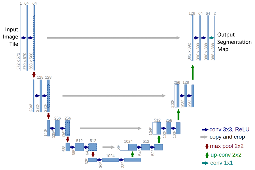
Figure 20.3: U-Net architecture
Object detection
The object detection task is similar to the classification and localization task. The big difference is that now there are multiple objects in the image, and for each one of them, we need to find the class and the bounding box coordinates. In addition, neither the number of objects nor their size is known in advance. As you can imagine, this is a difficult problem, and a fair amount of research has gone into it.
A first approach to the problem might be to create many random crops of the input image and, for each crop, apply the classification and localization network we described earlier. However, such an approach is very wasteful in terms of computing and unlikely to be very successful.
A more practical approach would be to use a tool such as Selective Search (Selective Search for Object Recognition, by Uijlings et al., http://www.huppelen.nl/publications/selectiveSearchDraft.pdf), which uses traditional computer vision techniques to find areas in the image that might contain objects. These regions are called “region proposals,” and the network to detect them is called Region-based CNN, or R-CNN. In the original R-CNN, the regions were resized and fed into a network to yield image vectors. These vectors were then classified with an SVM-based classifier (see https://en.wikipedia.org/wiki/Support-vector_machine), and the bounding boxes proposed by the external tool were corrected using a linear regression network over the image vectors. An R-CNN network can be represented conceptually as shown in Figure 20.4:
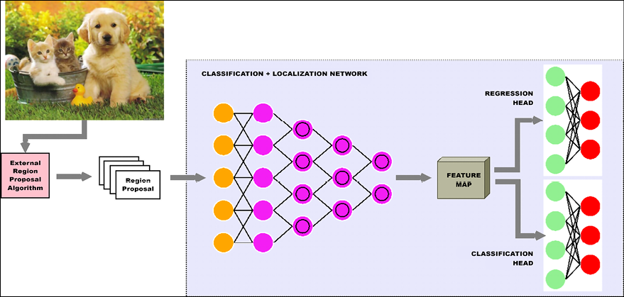
Figure 20.4: R-CNN network
The next iteration of the R-CNN network is called the Fast R-CNN. The Fast R-CNN still gets its region proposals from an external tool, but instead of feeding each region proposal through the CNN, the entire image is fed through the CNN and the region proposals are projected onto the resulting feature map. Each region of interest is fed through a Region Of Interest (ROI) pooling layer and then to a fully connected network, which produces a feature vector for the ROI.
ROI pooling is a widely used operation in object detection tasks using CNNs. The ROI pooling layer uses max pooling to convert the features inside any valid region of interest into a small feature map with a fixed spatial extent of H x W (where H and W are two hyperparameters). The feature vector is then fed into two fully connected networks, one to predict the class of the ROI and the other to correct the bounding box coordinates for the proposal. This is illustrated in Figure 20.5:
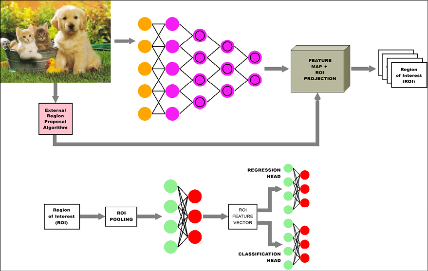
Figure 20.5: Fast R-CNN network architecture
The Fast R-CNN is about 25x faster than the R-CNN. The next improvement, called the Faster R-CNN (an implementation is at https://github.com/tensorpack/tensorpack/tree/master/examples/FasterRCNN), removes the external region proposal mechanism and replaces it with a trainable component, called the Region Proposal Network (RPN), within the network itself. The output of this network is combined with the feature map and passed in through a similar pipeline to the Fast R-CNN network, as shown in Figure 20.6.
The Faster R-CNN network is about 10x faster than the Fast R-CNN network, making it approximately 250x faster than an R-CNN network:
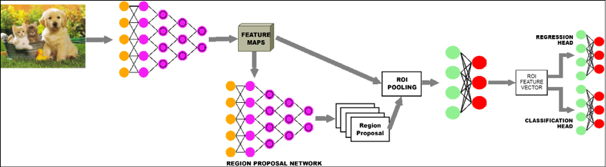
Figure 20.6: Faster R-CNN network architecture
Another somewhat different class of object detection networks are Single Shot Detectors (SSD) such as YOLO (You Only Look Once). In these cases, each image is split into a predefined number of parts using a grid. In the case of YOLO, a 7 x 7 grid is used, resulting in 49 sub-images. A predetermined set of crops with different aspect ratios are applied to each sub-image. Given B bounding boxes and C object classes, the output for each image is a vector of size  . Each bounding box has a confidence and coordinates (x, y, w, h), and each grid has prediction probabilities for the different objects detected within them.
The YOLO network is a CNN, which does this transformation. The final predictions and bounding boxes are found by aggregating the findings from this vector. In YOLO, a single convolutional network predicts the bounding boxes and the related class probabilities. YOLO is the faster solution for object detection. An implementation is at https://www.kaggle.com/aruchomu/yolo-v3-object-detection-in-tensorflow.
Instance segmentation
Instance segmentation is similar to semantic segmentation – the process of associating each pixel of an image with a class label – with a few important distinctions. First, it needs to distinguish between different instances of the same class in an image. Second, it is not required to label every single pixel in the image. In some respects, instance segmentation is also similar to object detection, except that instead of bounding boxes, we want to find a binary mask that covers each object.
The second definition leads to the intuition behind the Mask R-CNN network. The Mask R-CNN is a Faster R-CNN with an additional CNN in front of its regression head, which takes as input the bounding box coordinates reported for each ROI and converts it to a binary mask [11]:
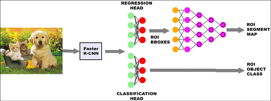
Figure 20.7: Mask R-CNN architecture
In April 2019, Google released Mask R-CNN in open source, pretrained with TPUs. This is available at
I suggest playing with the Colab notebook to see what the results are. In Figure 20.8, we see an example of image segmentation:

Figure 20.8: An example of image segmentation
Google also released another model trained on TPUs called DeepLab, and you can see an image (Figure 20.9) from the demo. This is available at

Figure 20.9: An example of image segmentation
In this section, we have covered, at a somewhat high level, various network architectures that are popular in computer vision. Note that all of them are composed by the same basic CNN and fully connected architectures. This composability is one of the most powerful features of deep learning. Hopefully, this has given you some ideas for networks that could be adapted for your own computer vision use cases.
Application zoos with tf.Keras and TensorFlow Hub
One of the nice things about transfer learning is that it is possible to reuse pretrained networks to save time and resources. There are many collections of ready-to-use networks out there, but the following two are the most used.
Keras Applications
Keras Applications (Keras Applications are available at https://www.tensorflow.org/api_docs/python/tf/keras/applications) includes models for image classification with weights trained on ImageNet (Xception, VGG16, VGG19, ResNet, ResNetV2, ResNeXt, InceptionV3, InceptionResNetV2, MobileNet, MobileNetV2, DenseNet, and NASNet). In addition, there are a few other reference implementations from the community for object detection and segmentation, sequence learning, reinforcement learning (see Chapter 11), and GANs (see Chapter 9).
TensorFlow Hub
TensorFlow Hub (available at https://www.tensorflow.org/hub) is an alternative collection of pretrained models. TensorFlow Hub includes modules for text classification, sentence encoding (see Chapter 4), image classification, feature extraction, image generation with GANs, and video classification. Currently, both Google and DeepMind contribute to TensorFlow Hub.
Let’s look at an example of using TF.Hub. In this case, we have a simple image classifier using MobileNetv2:
import matplotlib.pylab as plt
import tensorflow as tf
import tensorflow_hub as hub
import numpy as np
import PIL.Image as Image
classifier_url ="https://tfhub.dev/google/tf2-preview/mobilenet_v2/classification/2" #@param {type:"string"}
IMAGE_SHAPE = (224, 224)
# wrap the hub to work with tf.keras
classifier = tf.keras.Sequential([
    hub.KerasLayer(classifier_url, input_shape=IMAGE_SHAPE+(3,))
])
grace_hopper = tf.keras.utils.get_file('image.jpg','https://storage.googleapis.com/download.tensorflow.org/example_images/grace_hopper.jpg')
grace_hopper = Image.open(grace_hopper).resize(IMAGE_SHAPE)
grace_hopper = np.array(grace_hopper)/255.0
result = classifier.predict(grace_hopper[np.newaxis, ...])
predicted_class = np.argmax(result[0], axis=-1)
print (predicted_class)
Pretty simple indeed. Just remember to use hub.KerasLayer() for wrapping any Hub layer. In this section, we have discussed how to use TensorFlow Hub.
Next, we will focus on other CNN architectures.
Answering questions about images (visual Q&A)
One of the nice things about neural networks is that different media types can be combined together to provide a unified interpretation. For instance, Visual Question Answering (VQA) combines image recognition and text natural language processing. Training can use VQA (VQA is available at https://visualqa.org/), a dataset containing open-ended questions about images. These questions require an understanding of vision, language, and common knowledge to be answered. The following images are taken from a demo available at https://visualqa.org/.
Note the question at the top of the image, and the subsequent answers:
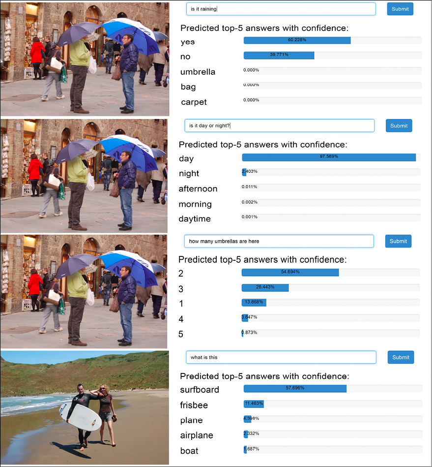
Figure 20.10: Examples of visual question and answers
If you want to start playing with VQA, the first thing is to get appropriate training datasets such as the VQA dataset, the CLEVR dataset (available at https://cs.stanford.edu/people/jcjohns/clevr/), or the FigureQA dataset (available at https://datasets.maluuba.com/FigureQA); alternatively, you can participate in a Kaggle VQA challenge (available at https://www.kaggle.com/c/visual-question-answering). Then you can build a model that is the combination of a CNN and an RNN and start experimenting. For instance, a CNN can be something like this code fragment, which takes an image with three channels (224 x 224) as input and produces a feature vector for the image:
import tensorflow as tf
from tensorflow.keras import layers, models
# IMAGE
#
# Define CNN for visual processing
cnn_model = models.Sequential()
cnn_model.add(layers.Conv2D(64, (3, 3), activation='relu', padding='same',
        input_shape=(224, 224, 3)))
cnn_model.add(layers.Conv2D(64, (3, 3), activation='relu'))
cnn_model.add(layers.MaxPooling2D(2, 2))
cnn_model.add(layers.Conv2D(128, (3, 3), activation='relu', padding='same'))
cnn_model.add(layers.Conv2D(128, (3, 3), activation='relu'))
cnn_model.add(layers.MaxPooling2D(2, 2))
cnn_model.add(layers.Conv2D(256, (3, 3), activation='relu', padding='same'))
cnn_model.add(layers.Conv2D(256, (3, 3), activation='relu'))
cnn_model.add(layers.Conv2D(256, (3, 3), activation='relu'))
cnn_model.add(layers.MaxPooling2D(2, 2))
cnn_model.add(layers.Flatten())
cnn_model.summary()
#define the visual_model with proper input
image_input = layers.Input(shape=(224, 224, 3))
visual_model = cnn_model(image_input)
Text can be encoded with an RNN; for now, think of it as a black box taking a text fragment (the question) in input and producing a feature vector for the text:
# TEXT
#
#define the RNN model for text processing
question_input = layers.Input(shape=(100,), dtype='int32')
emdedding = layers.Embedding(input_dim=10000, output_dim=256,
    input_length=100)(question_input)
encoded_question = layers.LSTM(256)(emdedding)
Then the two feature vectors (one for the image, and one for the text) are combined into one joint vector, which is provided as input to a dense network to produce the combined network:
# combine the encoded question and visual model
merged = layers.concatenate([encoded_question, visual_model])
#attach a dense network at the end
output = layers.Dense(1000, activation='softmax')(merged)
#get the combined model
vqa_model = models.Model(inputs=[image_input, question_input], outputs=output)
vqa_model.summary()
For instance, if we have a set of labeled images, then we can learn what the best questions and answers are for describing an image. The number of options is enormous! If you want to know more, I suggest that you investigate Maluuba, a start-up providing the FigureQA dataset with 100,000 figure images and 1,327,368 question-answer pairs in the training set. Maluuba has been recently acquired by Microsoft, and the lab is advised by Yoshua Bengio, one of the fathers of deep learning.
In this section, we have discussed how to implement visual Q&A. The next section is about style transfer, a deep learning technique used for training neural networks to create art.
Creating a DeepDream network
Another interesting application of CNNs is DeepDream, a computer vision program created by Google [8] that uses a CNN to find and enhance patterns in images. The result is a dream-like hallucinogenic effect. Similar to the previous example, we are going to use a pretrained network to extract features. However, in this case, we want to “enhance” patterns in images, meaning that we need to maximize some functions. This tells us that we need to use a gradient ascent and not a descent. First, let’s see an example from Google gallery (available at https://colab.research.google.com/github/tensorflow/docs/blob/master/site/en/tutorials/generative/deepdream.ipynb) where the classic Seattle landscape is “incepted” with hallucinogenic dreams such as birds, cards, and strange flying objects.
Google released the DeepDream code as open source (available at https://github.com/google/deepdream), but we will use a simplified example made by a random forest (available at https://www.tensorflow.org/tutorials/generative/deepdream):

Figure 20.11: DeepDreaming Seattle
Let’s start with some image preprocessing:
# Download an image and read it into a NumPy array,
def download(url):
  name = url.split("/")[-1]
  image_path = tf.keras.utils.get_file(name, origin=url)
  img = image.load_img(image_path)
  return image.img_to_array(img)
# Scale pixels to between (-1.0 and 1.0)
def preprocess(img):
  return (img / 127.5) - 1

# Undo the preprocessing above
def deprocess(img):
  img = img.copy()
  img /= 2.
  img += 0.5
  img *= 255.
  return np.clip(img, 0, 255).astype('uint8')
# Display an image
def show(img):
  plt.figure(figsize=(12,12))
  plt.grid(False)
  plt.axis('off')
  plt.imshow(img)
# https://commons.wikimedia.org/wiki/File:Flickr_-_Nicholas_T_-_Big_Sky_(1).jpg
url = 'https://upload.wikimedia.org/wikipedia/commons/thumb/d/d0/Flickr_-_Nicholas_T_-_Big_Sky_%281%29.jpg/747px-Flickr_-_Nicholas_T_-_Big_Sky_%281%29.jpg'
img = preprocess(download(url))
show(deprocess(img))
Now let’s use the Inception pretrained network to extract features. We use several layers, and the goal is to maximize their activations. The tf.keras functional API is our friend here:
# We'll maximize the activations of these layers
names = ['mixed2', 'mixed3', 'mixed4', 'mixed5']
layers = [inception_v3.get_layer(name).output for name in names]
# Create our feature extraction model
feat_extraction_model = tf.keras.Model(inputs=inception_v3.input, outputs=layers)
def forward(img):

  # Create a batch
  img_batch = tf.expand_dims(img, axis=0)

  # Forward the image through Inception, extract activations
  # for the layers we selected above
  return feat_extraction_model(img_batch)
The loss function is the mean of all the activation layers considered, normalized by the number of units in the layer itself:
def calc_loss(layer_activations):

  total_loss = 0

  for act in layer_activations:

    # In gradient ascent, we'll want to maximize this value
    # so our image increasingly "excites" the layer
    loss = tf.math.reduce_mean(act)
    # Normalize by the number of units in the layer
    loss /= np.prod(act.shape)
    total_loss += loss
  return total_loss
Now let’s run the gradient ascent:
img = tf.Variable(img)
steps = 400
for step in range(steps):

  with tf.GradientTape() as tape:
    activations = forward(img)
    loss = calc_loss(activations)

  gradients = tape.gradient(loss, img)
  # Normalize the gradients
  gradients /= gradients.numpy().std() + 1e-8

  # Update our image by directly adding the gradients
  img.assign_add(gradients)

  if step % 50 == 0:
    clear_output()
    print ("Step %d, loss %f" % (step, loss))
    show(deprocess(img.numpy()))
    plt.show()
# Let's see the result
clear_output()
show(deprocess(img.numpy()))
This transforms the image on the left into the psychedelic image on the right:

Figure 20.12: DeepDreaming of a green field with clouds
Inspecting what a network has learned
A particularly interesting research effort is being devoted to understand what neural networks are actually learning in order to be able to recognize images so well. This is called neural network “interpretability.” Activation atlases is a promising recent technique that aims to show the feature visualizations of averaged activation functions. In this way, activation atlases produce a global map seen through the eyes of the network. Let’s look at a demo available at https://distill.pub/2019/activation-atlas/:

Figure 20.13: Examples of inspections
In this image, an InceptionV1 network used for vision classification reveals many fully realized features, such as electronics, screens, a Polaroid camera, buildings, food, animal ears, plants, and watery backgrounds. Note that grid cells are labeled with the classification they give the most support for. Grid cells are also sized according to the number of activations that are averaged within. This representation is very powerful because it allows us to inspect the different layers of a network and how the activation functions fire in response to the input.
In this section, we have seen many techniques to process images with CNNs. Next, we’ll move on to video processing.
Video
In this section, we are going to discuss how to use CNNs with videos and the different techniques that we can use.
Classifying videos with pretrained nets in six different ways
Classifying videos is an area of active research because of the large amount of data needed for processing this type of media. Memory requirements are frequently reaching the limits of modern GPUs and a distributed form of training on multiple machines might be required. Researchers are currently exploring different directions of investigation, with increasing levels of complexity from the first approach to the sixth, as described below. Let’s review them:
- The first approach consists of classifying one video frame at a time by considering each one of them as a separate image processed with a 2D CNN. This approach simply reduces the video classification problem to an image classification problem. Each video frame “emits” a classification output, and the video is classified by taking into account the more frequently chosen category for each frame.
- The second approach consists of creating one single network where a 2D CNN is combined with an RNN (see Chapter 9, Generative Models). The idea is that the CNN will take into account the image components and the RNN will take into account the sequence information for each video. This type of network can be very difficult to train because of the very high number of parameters to optimize.
- The third approach is to use a 3D ConvNet, where 3D ConvNets are an extension of 2D ConvNets operating on a 3D tensor (time, image width, and image height). This approach is another natural extension of image classification. Again, 3D ConvNets can be hard to train.
- The fourth approach is based on a clever idea: instead of using CNNs directly for classification, they can be used for storing offline features for each frame in the video. The idea is that feature extraction can be made very efficient with transfer learning, as shown in a previous recipe. After all the features are extracted, they can be passed as a set of inputs into an RNN, which will learn sequences across multiple frames and emit the final classification.
- The fifth approach is a simple variant of the fourth, where the final layer is an MLP instead of an RNN. In certain situations, this approach can be simpler and less expensive in terms of computational requirements.
- The sixth approach is a variant of the fourth, where the phase of feature extraction is realized with a 3D CNN that extracts spatial and visual features. These features are then passed into either an RNN or an MLP.
Deciding upon the best approach is strictly dependent on your specific application, and there is no definitive answer. The first three approaches are generally more computationally expensive and less clever, while the last three approaches are less expensive, and they frequently achieve better performance.
So far, we have explored how CNNs can be used for image and video applications. In the next section, we will apply these ideas within a text-based context.
Text documents
What do text and images have in common? At first glance, very little. However, if we represent a sentence or a document as a matrix, then this matrix is not much different from an image matrix where each cell is a pixel. So, the next question is, how can we represent a piece of text as a matrix?
Well, it is pretty simple: each row of a matrix is a vector that represents a basic unit for the text. Of course, now we need to define what a basic unit is. A simple choice could be to say that the basic unit is a character. Another choice would be to say that a basic unit is a word; yet another choice is to aggregate similar words together and then denote each aggregation (sometimes called cluster or embedding) with a representative symbol.
Note that regardless of the specific choice adopted for our basic units, we need to have a 1:1 mapping from basic units into integer IDs so that the text can be seen as a matrix. For instance, if we have a document with 10 lines of text and each line is a 100-dimensional embedding, then we will represent our text with a matrix of 10 x 100. In this very particular “image,” a “pixel” is turned on if that sentence, X, contains the embedding, represented by position Y. You might also notice that a text is not really a matrix but more a vector because two words located in adjacent rows of text have very little in common. Indeed, this is a major difference when compared with images, where two pixels located in adjacent columns are likely to have some degree of correlation.
Now you might wonder: I understand that we represent the text as a vector but, in doing so, we lose the position of the words. This position should be important, shouldn’t it? Well, it turns out that in many real applications, knowing whether a sentence contains a particular basic unit (a char, a word, or an aggregate) or not is pretty useful information even if we don’t keep track of where exactly in the sentence this basic unit is located.
For instance, CNNs achieve pretty good results for sentiment analysis, where we need to understand if a piece of text has a positive or a negative sentiment; for spam detection, where we need to understand if a piece of text is useful information or spam; and for topic categorization, where we need to understand what a piece of text is all about. However, CNNs are not well suited for a Part of Speech (POS) analysis, where the goal is to understand what the logical role of every single word is (for example, a verb, an adverb, a subject, and so on). CNNs are also not well suited for entity extraction, where we need to understand where relevant entities are located in sentences.
Indeed, it turns out that a position is pretty useful information for the last two use cases. 1D ConvNets are very similar to 2D ConvNets. However, the former operates on a single vector, while the latter operates on matrices.
Using a CNN for sentiment analysis
Let’s have a look at the code. First of all, we load the dataset with tensorflow_datasets. In this case we use IMDB, a collection of movie reviews:
import tensorflow as tf
from tensorflow.keras import datasets, layers, models, preprocessing
import tensorflow_datasets as tfds
max_len = 200
n_words = 10000
dim_embedding = 256
EPOCHS = 20
BATCH_SIZE =500
def load_data():
    #load data
    (X_train, y_train), (X_test, y_test) = datasets.imdb.load_data(num_words=n_words)
    # Pad sequences with max_len
    X_train = preprocessing.sequence.pad_sequences(X_train, maxlen=max_len)
    X_test = preprocessing.sequence.pad_sequences(X_test, maxlen=max_len)
    return (X_train, y_train), (X_test, y_test)
Then we build a suitable CNN model. We use embeddings (see Chapter 4, Word Embeddings) to map the sparse vocabulary typically observed in documents into a dense feature space of dimensions dim_embedding. Then we use Conv1D, followed by a GlobalMaxPooling1D for averaging, and two Dense layers – the last one has only one neuron firing binary choices (positive or negative reviews):
def build_model():
    model = models.Sequential()
    #Input - Embedding Layer
    # the model will take as input an integer matrix of size (batch, input_length)
    # the model will output dimension (input_length, dim_embedding)
    # the largest integer in the input should be no larger
    # than n_words (vocabulary size).
    model.add(layers.Embedding(n_words,
        dim_embedding, input_length=max_len))
    model.add(layers.Dropout(0.3))
    model.add(layers.Conv1D(256, 3, padding='valid',
        activation='relu'))
    #takes the maximum value of either feature vector from each of the n_words features
    model.add(layers.GlobalMaxPooling1D())
    model.add(layers.Dense(128, activation='relu'))
    model.add(layers.Dropout(0.5))
    model.add(layers.Dense(1, activation='sigmoid'))
    return model
(X_train, y_train), (X_test, y_test) = load_data()
model=build_model()
model.summary()
The model has more than 2,700,000 parameters, and it is summarized as follows:
_________________________________________________________________
 Layer (type)                Output Shape              Param #
=================================================================
 embedding (Embedding)       (None, 200, 256)          2560000

 dropout (Dropout)           (None, 200, 256)          0

 conv1d (Conv1D)             (None, 198, 256)          196864

 global_max_pooling1d (Globa  (None, 256)              0
 lMaxPooling1D)

 dense (Dense)               (None, 128)               32896

 dropout_1 (Dropout)         (None, 128)               0

 dense_1 (Dense)             (None, 1)                 129

=================================================================
Total params: 2,789,889
Trainable params: 2,789,889
Non-trainable params: 0
Then we compile and fit the model with the Adam optimizer and binary cross-entropy loss:
model.compile(optimizer = "adam", loss = "binary_crossentropy",
  metrics = ["accuracy"]
)
score = model.fit(X_train, y_train,
  epochs= EPOCHS,
  batch_size = BATCH_SIZE,
  validation_data = (X_test, y_test)
)
score = model.evaluate(X_test, y_test, batch_size=BATCH_SIZE)
print("
Test score:", score[0])
print('Test accuracy:', score[1])
The final accuracy is 88.21%, showing that it is possible to successfully use CNNs for textual processing:
Epoch 19/20
25000/25000 [==============================] - 135s 5ms/sample - loss: 7.5276e-04 - accuracy: 1.0000 - val_loss: 0.5753 - val_accuracy: 0.8818
Epoch 20/20
25000/25000 [==============================] - 129s 5ms/sample - loss: 6.7755e-04 - accuracy: 0.9999 - val_loss: 0.5802 - val_accuracy: 0.8821
25000/25000 [==============================] - 23s 916us/sample - loss: 0.5802 - accuracy: 0.8821
Test score: 0.5801781857013703
Test accuracy: 0.88212
Note that many other non-image applications can also be converted to an image and classified using CNNs (see, for instance, https://becominghuman.ai/sound-classification-using-images-68d4770df426).
Audio and music
We have used CNNs for images, videos, and texts. Now let’s have a look at how variants of CNNs can be used for audio.
So, you might wonder why learning to synthesize audio is so difficult. Well, each digital sound we hear is based on 16,000 samples per second (sometimes 48K or more), and building a predictive model where we learn to reproduce a sample based on all the previous ones is a very difficult challenge.
Dilated ConvNets, WaveNet, and NSynth
WaveNet is a deep generative model for producing raw audio waveforms. This breakthrough technology was introduced (available at https://deepmind.com/blog/wavenet-a-generative-model-for-raw-audio/) by Google DeepMind for teaching computers how to speak. The results are truly impressive, and online you can find examples of synthetic voices where the computer learns how to talk with the voice of celebrities such as Matt Damon. There are experiments showing that WaveNet improved the current state-of-the-art Text-to-Speech (TTS) systems, reducing the difference with respect to human voices by 50% for both US English and Mandarin Chinese. The metric used for comparison is called Mean Opinion Score (MOS), a subjective paired comparison test. In the MOS tests, after listening to each sound stimulus, the subjects were asked to rate the naturalness of the stimulus on a five-point scale from “Bad” (1) to “Excellent” (5).
What is even cooler is that DeepMind demonstrated that WaveNet can be also used to teach computers how to generate the sound of musical instruments such as piano music.
Now some definitions. TTS systems are typically divided into two different classes: concatenative and parametric.
Concatenative TTS is where single speech voice fragments are first memorized and then recombined when the voice has to be reproduced. However, this approach does not scale because it is possible to reproduce only the memorized voice fragments, and it is not possible to reproduce new speakers or different types of audio without memorizing the fragments from the beginning.
Parametric TTS is where a model is created to store all the characteristic features of the audio to be synthesized. Before WaveNet, the audio generated with parametric TTS was less natural than concatenative TTS. WaveNet enabled significant improvement by modeling directly the production of audio sounds, instead of using intermediate signal processing algorithms as in the past.
In principle, WaveNet can be seen as a stack of 1D convolutional layers with a constant stride of one and with no pooling layers. Note that the input and the output have by construction the same dimension, so ConvNets are well suited to modeling sequential data such as audio sounds. However, it has been shown that in order to reach a large size for the receptive field in the output neuron, it is necessary to either use a massive number of large filters or increase the network depth prohibitively. Remember that the receptive field of a neuron in a layer is the cross-section of the previous layer from which neurons provide inputs. For this reason, pure ConvNets are not so effective in learning how to synthesize audio.
The key intuition behind WaveNet is the so-called Dilated Causal Convolutions [5] (sometimes called atrous convolution), which simply means that some input values are skipped when the filter of a convolutional layer is applied. “Atrous” is a “bastardization” of the French expression “à trous,” meaning “with holes.” So an atrous convolution is a convolution with holes. As an example, in one dimension, a filter w of size 3 with a dilation of 1 would compute the following sum: w[0] x[0] + w[1] x[2] + w[3] x[4].
In short, in D-dilated convolution, usually the stride is 1, but nothing prevents you from using other strides. An example is given in Figure 20.14 with increased dilatation (hole) sizes = 0, 1, 2:

Figure 20.14: Dilatation with increased sizes
Thanks to this simple idea of introducing holes, it is possible to stack multiple dilated convolutional layers with exponentially increasing filters and learn long-range input dependencies without having an excessively deep network.
A WaveNet is therefore a ConvNet where the convolutional layers have various dilation factors, allowing the receptive field to grow exponentially with depth and therefore efficiently cover thousands of audio timesteps.
When we train, the inputs are sounds recorded from human speakers. The waveforms are quantized to a fixed integer range. A WaveNet defines an initial convolutional layer accessing only the current and previous input. Then, there is a stack of dilated ConvNet layers, still accessing only current and previous inputs. At the end, there is a series of dense layers combining previous results, followed by a softmax activation function for categorical outputs.
At each step, a value is predicted from the network and fed back into the input. At the same time, a new prediction for the next step is computed. The loss function is the cross-entropy between the output for the current step and the input at the next step. Figure 20.15 shows the visualization of a WaveNet stack and its receptive field as introduced in Aaron van den Oord [9]. Note that generation can be slow because the waveform has to be synthesized in a sequential fashion, as xt must be sampled first in order to obtain  where x is the input:
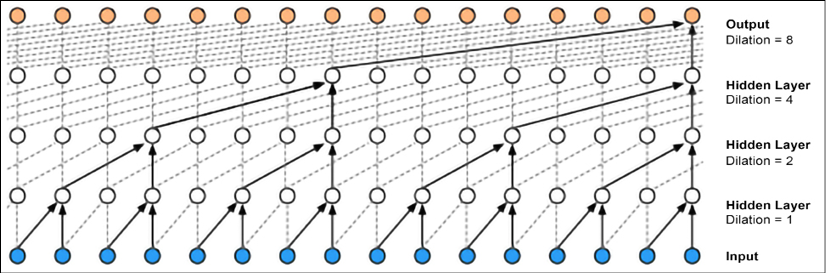
Figure 20.15: WaveNet internal connections
A method for performing a sampling in parallel has been proposed in Parallel WaveNet [10], which achieves a three orders-of-magnitude speedup. This uses two networks as a WaveNet teacher network, which is slow but ensures a correct result, and a WaveNet student network, which tries to mimic the behavior of the teacher; this can prove to be less accurate but is faster. This approach is similar to the one used for GANs (see Chapter 9, Generative Models) but the student does not try to fool the teacher, as typically happens in GANs. In fact, the model is not just quicker but also of higher fidelity, capable of creating waveforms with 24,000 samples per second:
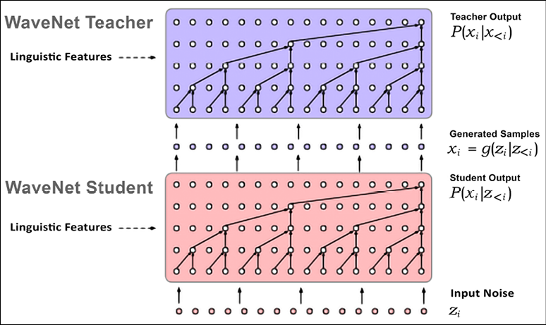
Figure 20.16: Examples of WaveNet Student and Teacher
This model has been deployed in production at Google, and is currently being used to serve Google Assistant queries in real time to millions of users. At the annual I/O developer conference in May 2018, it was announced that new Google Assistant voices were available thanks to WaveNet.
Two implementations of WaveNet models for TensorFlow are currently available. One is the original implementation of DeepMind’s WaveNet, and the other is called Magenta NSynth. The original WaveNet version is available at https://github.com/ibab/tensorflow-wavenet. NSynth is an evolution of WaveNet recently released by the Google Brain group, which, instead of being causal, aims at seeing the entire context of the input chunk. Magenta is available at https://magenta.tensorflow.org/nsynth.
The neural network is truly complex, as depicted in the image below, but for the sake of this introductory discussion, it is sufficient to know that the network learns how to reproduce its input by using an approach based on reducing the error during the encoding/decoding phases:
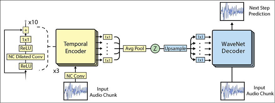
Figure 20.17: Magenta internal architecture
If you are interested in understanding more, I would suggest having a look at the online Colab notebook where you can play with models generated with NSynth. NSynth Colab is available at https://colab.research.google.com/notebooks/magenta/nsynth/nsynth.ipynb.
MuseNet is a very recent and impressive cool audio generation tool developed by OpenAI. MuseNet uses a sparse transformer to train a 72-layer network with 24 attention heads. MuseNet is available at https://openai.com/blog/musenet/. Transformers, discussed in Chapter 6, are very good at predicting what comes next in a sequence – whether text, images, or sound.
In transformers, every output element is connected to every input element, and the weightings between them are dynamically calculated according to a process called attention. MuseNet can produce up to 4-minute musical compositions with 10 different instruments, and can combine styles from country, to Mozart, to the Beatles. For instance, I generated a remake of Beethoven’s “Für Elise” in the style of Lady Gaga with piano, drums, guitar, and bass. You can try this for yourself at the link provided under the section Try MuseNet:
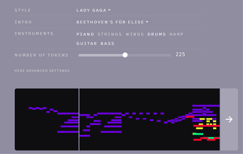
Figure 20.18: An example of using MuseNet
A summary of convolution operations
In this section, we present a summary of different convolution operations. A convolutional layer has I input channels and produces O output channels. I x O x K parameters are used, where K is the number of values in the kernel.
Basic CNNs
Let’s remind ourselves briefly what a CNN is. CNNs take in an input image (two dimensions), text (two dimensions), or video (three dimensions) and apply multiple filters to the input. Each filter is like a flashlight sliding across the areas of the input, and the areas that it is shining over are called the receptive field. Each filter is a tensor of the same depth of the input (for instance, if the image has a depth of three, then the filter must also have a depth of three).
When the filter is sliding, or convolving, around the input image, the values in the filter are multiplied by the values of the input. The multiplications are then summarized into one single value. This process is repeated for each location, producing an activation map (a.k.a. a feature map). Of course, it is possible to use multiple filters where each filter will act as a feature identifier. For instance, for images, the filter can identify edges, colors, lines, and curves. The key intuition is to treat the filter values as weights and fine-tune them during training via backpropagation.
A convolution layer can be configured by using the following config parameters:
- Kernel size: This is the field of view of the convolution.
- Stride: This is the step size of the kernel when we traverse the image.
- Padding: Defines how the border of our sample is handled.
Dilated convolution
Dilated convolutions (or atrous convolutions) introduce another config parameter:
Dilated convolutions are used in many contexts including audio processing with WaveNet.
Transposed convolution
Transposed convolution is a transformation going in the opposite direction of a normal convolution. For instance, this can be useful to project feature maps into a higher dimensional space or for building convolutional autoencoders (see Chapter 8, Autoencoders). One way to think about transposed convolution is to compute the output shape of a normal CNN for a given input shape first. Then we invert input and output shapes with the transposed convolution. TensorFlow 2.0 supports transposed convolutions with Conv2DTranspose layers, which can be used, for instance, in GANs (see Chapter 9, Generative Models) for generating images.
Separable convolution
Separable convolution aims at separating the kernel in multiple steps. Let the convolution be y = conv(x, k) where y is the output, x is the input, and k is the kernel. Let’s assume the kernel is separable, k = k1.k2 where . is the dot product – in this case, instead of doing a 2-dimension convolution with k, we can get to the same result by doing two 1-dimension convolutions with k1 and k2. Separable convolutions are frequently used to save on computation resources.
Depthwise convolution
Let’s consider an image with multiple channels. In the normal 2D convolution, the filter is as deep as the input, and it allows us to mix channels for generating each element of the output. In depthwise convolutions, each channel is kept separate, the filter is split into channels, each convolution is applied separately, and the results are stacked back together into one tensor.
Depthwise separable convolution
This convolution should not be confused with the separable convolution. After completing the depthwise convolution, an additional step is performed: a 1x1 convolution across channels. Depthwise separable convolutions are used in Xception. They are also used in MobileNet, a model particularly useful for mobile and embedded vision applications because of its reduced model size and complexity.
In this section, we have discussed all the major forms of convolution. The next section will discuss capsule networks, a new form of learning introduced in 2017.
Capsule networks
Capsule networks (or CapsNets) are a very recent and innovative type of deep learning network. This technique was introduced at the end of October 2017 in a seminal paper titled Dynamic Routing Between Capsules by Sara Sabour, Nicholas Frost, and Geoffrey Hinton (https://arxiv.org/abs/1710.09829) [14]. Hinton is the father of deep learning and, therefore, the whole deep learning community is excited to see the progress made with Capsules. Indeed, CapsNets are already beating the best CNN on MNIST classification, which is... well, impressive!!
What is the problem with CNNs?
In CNNs, each layer “understands” an image at a progressive level of granularity. As we discussed in multiple sections, the first layer will most likely recognize straight lines or simple curves and edges, while subsequent layers will start to understand more complex shapes such as rectangles up to complex forms such as human faces.
Now, one critical operation used for CNNs is pooling. Pooling aims at creating positional invariance and it is used after each CNN layer to make any problem computationally tractable. However, pooling introduces a significant problem because it forces us to lose all the positional data. This is not good. Think about a face: it consists of two eyes, a mouth, and a nose, and what is important is that there is a spatial relationship between these parts (for example, the mouth is below the nose, which is typically below the eyes). Indeed, Hinton said: The pooling operation used in convolutional neural networks is a big mistake and the fact that it works so well is a disaster. Technically, we do not need positional invariance but instead we need equivariance. Equivariance is a fancy term for indicating that we want to understand the rotation or proportion change in an image, and we want to adapt the network accordingly. In this way, the spatial positioning among the different components in an image is not lost.
What is new with capsule networks?
According to Hinton et al., our brain has modules called “capsules,” and each capsule is specialized in handling a particular type of information. In particular, there are capsules that work well for “understanding” the concept of position, the concept of size, the concept of orientation, the concept of deformation, textures, and so on. In addition to that, the authors suggest that our brain has particularly efficient mechanisms for dynamically routing each piece of information to the capsule that is considered best suited for handling a particular type of information.
So, the main difference between CNN and CapsNets is that with a CNN, we keep adding layers for creating a deep network, while with CapsNet, we nest a neural layer inside another. A capsule is a group of neurons that introduces more structure to a network, and it produces a vector to signal the existence of an entity in an image. In particular, Hinton uses the length of the activity vector to represent the probability that the entity exists and its orientation to represent the instantiation parameters. When multiple predictions agree, a higher-level capsule becomes active. For each possible parent, the capsule produces an additional prediction vector.
Now a second innovation comes in place: we will use dynamic routing across capsules and will no longer use the raw idea of pooling. A lower-level capsule prefers to send its output to higher-level capsules for which the activity vectors have a big scalar product, with the prediction coming from the lower-level capsule. The parent with the largest scalar prediction vector product increases the capsule bond. All the other parents decrease their bond. In other words, the idea is that if a higher-level capsule agrees with a lower-level one, then it will ask to send more information of that type. If there is no agreement, it will ask to send fewer of them. This dynamic routing by the agreement method is superior to the current mechanism like max pooling and, according to Hinton, routing is ultimately a way to parse the image. Indeed, max pooling is ignoring anything but the largest value, while dynamic routing selectively propagates information according to the agreement between lower layers and upper layers.
A third difference is that a new nonlinear activation function has been introduced. Instead of adding a squashing function to each layer as in CNN, CapsNet adds a squashing function to a nested set of layers. The nonlinear activation function is represented in Equation 1, and it is called the squashing function:

where vj is the vector output of capsule j and sj is its total input.
Moreover, Hinton and others show that a discriminatively trained, multi-layer capsule system achieves state-of-the-art performances on MNIST and is considerably better than a convolutional net at recognizing highly overlapping digits.
Based on the paper Dynamic Routing Between Capsules, a simple CapsNet architecture looks as follows:
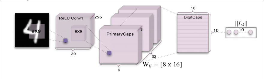
Figure 20.19: An example of CapsNet
The architecture is shallow with only two convolutional layers and one fully connected layer. Conv1 has 256 9 x 9 convolution kernels with a stride of 1 and ReLU activation. The role of this layer is to convert pixel intensities to the activities of local feature detectors that are then used as inputs to the PrimaryCapsules layer. PrimaryCapsules is a convolutional capsule layer with 32 channels; each primary capsule contains 8 convolutional units with a 9 x 9 kernel and a stride of 2. In total, PrimaryCapsules has [32, 6, 6] capsule outputs (each output is an 8D vector) and each capsule in the [6, 6] grid shares its weights with each other. The final layer (DigitCaps) has one 16D capsule per digit class and each one of these capsules receives input from all the other capsules in the layer below. Routing happens only between two consecutive capsule layers (for example, PrimaryCapsules and DigitCaps).
Summary
In this chapter, we have seen many applications of CNNs across very different domains, from traditional image processing and computer vision to close-enough video processing, not-so-close audio processing, and text processing. In just a few years, CNNs have taken machine learning by storm.
Nowadays, it is not uncommon to see multimodal processing, where text, images, audio, and videos are considered together to achieve better performance, frequently by means of combining CNNs together with a bunch of other techniques such as RNNs and reinforcement learning. Of course, there is much more to consider, and CNNs have recently been applied to many other domains such as genetic inference [13], which are, at least at first glance, far away from the original scope of their design.
References
- Yosinski, J. and Clune, Y. B. J. How transferable are features in deep neural networks. Advances in Neural Information Processing Systems 27, pp. 3320–3328.
- Szegedy, C., Vanhoucke, V., Ioffe, S., Shlens, J., and Wojna, Z. (2016). Rethinking the Inception Architecture for Computer Vision. 2016 IEEE Conference on Computer Vision and Pattern Recognition (CVPR), pp. 2818–2826.
- Sandler, M., Howard, A., Zhu, M., Zhmonginov, A., and Chen, L. C. (2019). MobileNetV2: Inverted Residuals and Linear Bottlenecks. Google Inc.
- Krizhevsky, A., Sutskever, I., Hinton, G. E., (2012). ImageNet classification with deep convolutional neural networks.
- Huang, G., Liu, Z., van der Maaten, L., and Weinberger, K. Q. (28 Jan 2018). Densely Connected Convolutional Networks. http://arxiv.org/abs/1608.06993
- Chollet, F. (2017). Xception: Deep Learning with Depthwise Separable Convolutions. https://arxiv.org/abs/1610.02357
- Gatys, L. A., Ecker, A. S., and Bethge, M. (2016). A Neural Algorithm of Artistic Style. https://arxiv.org/abs/1508.06576
- Mordvintsev, A., Olah, C., and Tyka, M. ( 2015). DeepDream - a code example for visualizing Neural Networks. Google Research.
- van den Oord, A., Dieleman, S., Zen, H., Simonyan, K., Vinyals, O., Graves, A., Kalchbrenner, N., Senior, A., and Kavukcuoglu, K. (2016). WaveNet: A generative model for raw audio. arXiv preprint.
- van den Oord, A., Li, Y., Babuschkin, I., Simonyan, K., Vinyals, O., Kavukcuoglu, K., van den Driessche, G., Lockhart, E., Cobo, L. C., Stimberg, F., Casagrande, N., Grewe, D., Noury, S., Dieleman, S., Elsen, E., Kalchbrenner, N., Zen, H., Graves, A., King, H., Walters, T., Belov, D., and Hassabis, D. (2017). Parallel WaveNet: Fast High-Fidelity Speech Synthesis.
- He, K., Gkioxari, G., Dollár, P., and Girshick, R. (2018). Mask R-CNN.
- Chen, L-C., Zhu, Y., Papandreou, G., Schroff, F., and Adam, H. (2018). Encoder-Decoder with Atrous Separable Convolution for Semantic Image Segmentation.
- Flagel, L., Brandvain, Y., and Schrider, D.R. (2018). The Unreasonable Effectiveness of Convolutional Neural Networks in Population Genetic Inference.
- Sabour, S., Frosst, N., and Hinton, G. E. (2017). Dynamic Routing Between Capsules https://arxiv.org/abs/1710.09829
Join our book’s Discord space
Join our Discord community to meet like-minded people and learn alongside more than 2000 members at: https://packt.link/keras
