14

Mastering Sharding

Sharding is the ability to horizontally scale out our database by partitioning our datasets across different servers—shards. This has been a feature of MongoDB since version 1.6 (v1.6) was released in August 2010. Foursquare and Bitly are two of MongoDB’s most famous early customers and have used the sharding feature from its inception all the way to its general release.

In this chapter, we will learn about the following topics:

• How to design a sharding cluster and how to make the important decision of choosing the shard key
• Different sharding techniques and how to monitor and administrate sharded clusters
• The mongos router and how it is used to route our queries across different shards
• How we can recover from errors in our shards

By the end of this chapter, we will have mastered the underlying theory and concepts as well as the practical implementation of sharding using MongoDB.

This chapter covers the following topics:

• Why do we need sharding?
• Architectural overview
• Setting up sharding
• Sharding administration and monitoring
• Querying sharded data
• Sharding recovery

Technical requirements

To follow along with the code in this chapter, you need to connect to a MongoDB Atlas database. You can use the fully managed database-as-a-service (DBaaS) MongoDB Atlas offering, which provides a free tier as well as seamless upgrades to the latest version. You may need to switch to a paid plan to access the full range of sharding features on the MongoDB Atlas platform.

Why do we need sharding?

In database systems and computing systems in general, we have two ways to improve performance. The first one is to simply replace our servers with more powerful ones, keeping the same network topology and systems architecture. This is called vertical scaling.

An advantage of vertical scaling is that it is simple, from an operational standpoint, especially with cloud providers such as Amazon making it a matter of a few clicks to replace an r6g.medium server instance with an r6g.extralarge one. Another advantage is that we don’t need to make any code changes, so there is little to no risk of something going catastrophically wrong.

The main disadvantage of vertical scaling is that there is a limit to it; we can only get servers that are as powerful as those our cloud provider can give to us.

A related disadvantage is that getting more powerful servers generally comes with an increase in cost that is not linear but exponential. So, even if our cloud provider offers more powerful instances, we will hit the cost-effectiveness barrier before we hit the limit of our department’s credit card.

The second way to improve performance is by using the same servers with the same capacity and increasing their number. This is called horizontal scaling.

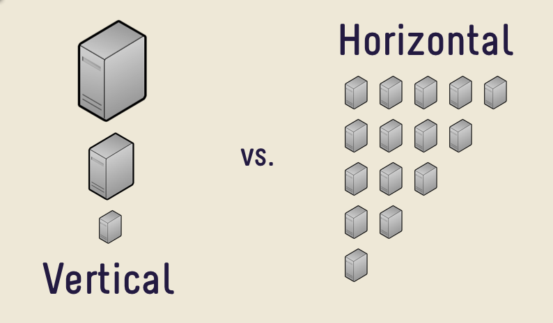
Horizontal scaling offers the advantage of theoretically being able to scale exponentially while remaining practical enough for real-world applications. The main disadvantage is that it can be operationally more complex and requires code changes and careful design of the system upfront. Horizontal scaling is also more complex when it comes to the system because it requires communication between the different servers over network links that are not as reliable as inter-process communication (IPC) on a single server. The following diagram shows the difference between horizontal and vertical scaling:

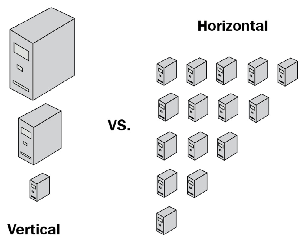
Figure 14.1: Conceptual architecture of vertical and horizontal scaling

To understand scaling, it’s important to understand the limitations of single-server systems. A server is typically bound by one or more of the following characteristics:

• Central processing unit (CPU): A CPU-bound system is one that is limited by our CPU’s speed. A task such as the multiplication of matrices that can fit in random-access memory (RAM) will be CPU bound because there is a specific number of steps that have to be performed in the CPU without any disk or memory access needed for the task to complete. In this case, CPU usage is the metric that we need to keep track of.
• Input/output (I/O): I/O-bound systems are similarly limited by the speed of our storage system (hard-disk drive (HDD) or solid-state drive (SSD)). A task such as reading large files from a disk to load into memory will be I/O bound as there is little to do in terms of CPU processing; a great majority of the time is spent reading files from the disk. The important metrics to keep track of are all metrics related to disk access, reads per second, and writes per second, compared to the practical limit of our storage system.
• Memory and cache: Memory-bound and cache-bound systems are restricted by the amount of available RAM and/or the cache size that we have assigned to them. A task that multiplies matrices larger than our RAM size will be memory bound, as it will need to page in/out data from the disk to perform the multiplication. The important metric to keep track of is the memory used. This may be misleading in MongoDB Memory Mapped Storage Engine v1 (MMAPv1), as the storage engine will allocate as much memory as possible through the filesystem cache.

In the WiredTiger storage engine, on the other hand, if we don’t allocate enough memory for the core MongoDB process, out-of-memory (OOM) errors may kill it, and this is something we want to avoid at all costs.

Monitoring memory usage has to be done both directly through the operating system and indirectly by keeping a track of page-in/out data. An increasing memory paging number is often an indication that we are running short of memory and the operating system is using virtual address space to keep up.

Note

MongoDB, being a database system, is generally memory and I/O bound. Investing in an SSD and more memory for our nodes is almost always a good investment. Most systems are a combination of one or more of the preceding limitations. Once we add more memory, our system may become CPU bound, as complex operations are almost always a combination of CPU, I/O, and memory usage.

MongoDB’s sharding is simple enough to set up and operate, and this has contributed to its huge success over the years as it provides the advantages of horizontal scaling without requiring a large commitment of engineering and operations resources.

That being said, it’s really important to get sharding right from the beginning, as it is extremely difficult from an operational standpoint to change the configuration once it has been set up. As we will learn in the following sections, sharding should not be an afterthought, but rather a key architectural design decision from an early point in the design process.

Architectural overview

A sharded cluster is comprised of the following elements:

• Two or more shards. Each shard must be a replica set.
• One or more query routers (mongos). A mongos router provides an interface between our application and the database.
• A replica set of config servers. Config servers store metadata and configuration settings for the entire cluster.

The relationships between these elements are shown in the following diagram:

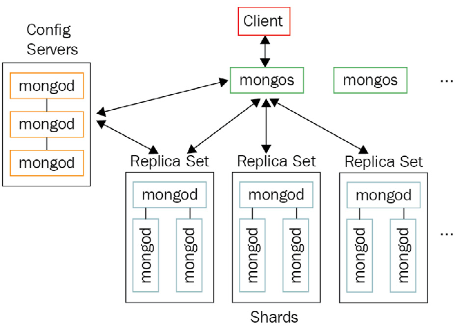
Figure 14.2: MongoDB sharded cluster architecture

Starting from MongoDB 3.6, shards must be implemented as replica sets.

Development, continuous deployment, and staging environments

In preproduction environments, it may be overkill to use the full set of servers. For efficiency reasons, we may opt to use a more simplified architecture.

The simplest possible configuration that we can deploy for sharding is the following:

• One mongos router
• One sharded replica set with one MongoDB server and two arbiters
• One replica set of config servers with three MongoDB servers

Support for multiple arbiters has been turned off by default in MongoDB 5.3. To enable it, we need to start each data server in the replica set with the allowMultipleArbiters=true parameter. Arbiters vote for successful operations but do not hold any data. So, for example, a write operation with write concern “majority” could succeed even when in our case we only have one data-bearing node and two arbiter nodes. Another potential issue is that when we change the replica set configuration using rs.reconfig() and we have multiple arbiters, the votes from multiple arbiters could elect as primary a node that has fallen behind in replication.

For these reasons, this configuration should only be used in development and staging environments and not in a production system.

A replica set of config servers must not have any delayed members or arbiters. All config servers must be configured to build indexes—this is enabled by default.

Staging is strongly recommended to mirror our production environment in terms of its servers, configuration, and (if possible) the stored dataset characteristics as well, in order to avoid surprises at deployment time.

Planning ahead with sharding

As we will see in the next sections, sharding is complicated and expensive, operation-wise. It is important to plan ahead and make sure that we start the sharding process long before we hit our system’s limits.

Some rough guidelines on when you need to start sharding are provided here:

• When you have a CPU utilization of less than 70% on average
• When I/O (and, especially, write) capacity is less than 80%
• When memory utilization is less than 70% on average

As sharding helps with write performance, it’s important to keep an eye on our I/O write capacity and the requirements of our application.

Note

Don’t wait until the last minute to start sharding in an already busy-up-to-the-neck MongoDB system, as this can have unintended consequences.

Setting up sharding

Sharding is performed at the collection level. We can have collections that we don’t want or need to shard for several reasons. We can leave these collections unsharded.

These collections will be stored in the primary shard. The primary shard is different for each database in MongoDB. The primary shard is automatically selected by MongoDB when we create a new database in a sharded environment. MongoDB will pick the shard that has the least data stored at the moment of creation.

If we want to change the primary shard at any other point, we can issue the following command:

> db.runCommand( { movePrimary : "mongo_books", to : "UK_based" } )

With this, we move the database named mongo_books to the shard named UK_based.

Choosing the shard key

Choosing our shard key is the most important decision we need to make: once we shard our data and deploy our cluster, it becomes very difficult to change the shard key. First, we will go through the process of changing the shard key.

Changing the shard key prior to v4.2

Prior to MongoDB v4.2, there was no command or simple procedure to change the shard key in MongoDB. The only way to change the shard key involved backing up and restoring all of our data, something that may range from being extremely difficult to impossible in high-load production environments.

Here are the steps that we need to go through in order to change the shard key:

1. Export all data from MongoDB.
2. Drop the original sharded collection.
3. Configure sharding with the new key.
4. Pre-split the new shard key range.
5. Restore our data back into MongoDB.

Of these steps, step 4 is the one that needs further explanation.

MongoDB uses chunks to split data in a sharded collection. If we bootstrap a MongoDB sharded cluster from scratch, chunks will be calculated automatically by MongoDB. MongoDB will then distribute the chunks across different shards to ensure that there is an equal number of chunks in each shard.

The only time when we cannot really do this is when we want to load data into a newly sharded collection.

The reasons for this are threefold, as explained here:

• MongoDB creates splits only after an insert operation.
• Chunk migration will copy all of the data in that chunk from one shard to another.
• floor(n/2) chunk migrations can happen at any given time, where n is the number of shards we have. Even with three shards, this is only a floor(1.5)=1 chunk migration at a time.

These three limitations mean that letting MongoDB figure it out on its own will definitely take much longer, and may result in an eventual failure. This is why we want to pre-split our data and give MongoDB some guidance on where our chunks should go.

In our example of the mongo_books database and the books collection, this is how it would look:

> db.runCommand( { split : "mongo_books.books", middle : { id : 50 } } )

The middle command parameter will split our key space into documents that have an id value less than or equal to 50 and documents that have an id value greater than 50. There is no need for a document to exist in our collection with an id value that is equal to 50 as this will only serve as the guidance value for our partitions.

In this example, we chose 50, as we assume that our keys follow a uniform distribution (that is, there is the same count of keys for each value) in the range of values from 0 to 100.

Note

We should aim to create at least 20-30 chunks to grant MongoDB flexibility in potential migrations. We can also use bounds and find instead of middle if we want to manually define the partition key, but both parameters need data to exist in our collection before applying them.

Changing the shard key – MongoDB v5, v6, and beyond

MongoDB v4.2 allowed users to modify a shard key’s value. MongoDB v4.4 allowed users to add a suffix to an existing shard key.

MongoDB v5.0 introduced live resharding, allowing users to change the shard key using a simple administrative command, as shown here:

sh.reshardCollection("<database>.<collection>", "<new_shardkey>")

We need to have at least 1.2 times the storage size of the collection for this operation to succeed. For example, if we reshard a collection that is 100 gigabytes (GB) in size, we need to make sure that we have at least 120 GB of free space across the cluster.

MongoDB recommends that CPU usage is less than 80% and I/O usage less than 50% before we attempt to reshard a collection.

Our application should be able to tolerate writes waiting for up to 2 seconds before being acknowledged while the resharding operation is in progress.

No index builds should be in progress before invoking the resharding command.

We should be cautious before invoking data definition-altering commands while resharding is in progress—these include, for example, index maintenance and collection definition changes. For example, changing the collection name while resharding this collection is not allowed, for good reasons.

Application code should be able to use both the current shard key and the new shard key if we want to ensure application availability while the resharding process is in progress.

Changing the shard key is administratively easy, but operationally heavy. Good shard key design is still needed, and that’s what we are going to learn how to do in the next section.

Choosing the correct shard key

After the previous section, it’s now self-evident that we need to take the choice of our shard key into consideration as this is a decision that we have to stick with.

A great shard key has the following three characteristics:

• High cardinality
• Low frequency
• Nonmonotonically changing values

We will go over the definitions of these three properties first to understand what they mean, as follows:

• High cardinality: This means that the shard key must have as many distinct values as possible. A Boolean can take only the values of true/false, and so it is a bad shard-key choice. A 64-bit long value field that can take any value from −(2^63) to 2^63−1 is a good shard-key choice, in terms of cardinality.
• Low frequency: This directly relates to the argument about high cardinality. A low-frequency shard key will have a distribution of values as close to a perfectly random/uniform distribution. Using the example of our 64-bit long value, it is of little use to us if we have a field that can take values ranging from −(2^63) to 2^63−1 if we end up observing the values of 0 and 1 all the time. In fact, it is as bad as using a Boolean field, which can also take only two values. If we have a shard key with high-frequency values, we will end up with chunks that are indivisible. These chunks cannot be further divided and will grow in size, negatively affecting the performance of the shard that contains them.
• Nonmonotonically changing values: This means that our shard key should not be, for example, an integer that always increases with every new insert. If we choose a monotonically increasing value as our shard key, this will result in all writes ending up in the last of all of our shards, limiting our write performance.

Note

If we want to use a monotonically changing value as the shard key, we should consider using hash-based sharding.

In the next section, we will describe different sharding strategies, including their advantages and disadvantages.

Range-based sharding

The default and most widely used sharding strategy is range-based sharding. This strategy will split our collection’s data into chunks, grouping documents with nearby values in the same shard.

For our example database and collection (mongo_books and books, respectively), we have the following:

> sh.shardCollection("mongo_books.books", { id: 1 } )

This creates a range-based shard key on id with an ascending direction. The direction of our shard key will determine which documents will end up in the first shard and which ones will appear in subsequent ones.

This is a good strategy if we plan to have range-based queries, as these will be directed to the shard that holds the result set instead of having to query all shards.

Hash-based sharding

If we don’t have a shard key (or can’t create one) that achieves the three goals mentioned previously, we can use the alternative strategy of hash-based sharding. In this case, we are trading data distribution with query isolation.

Hash-based sharding will take the values of our shard key and hash them in a way that guarantees close to uniform distribution. This way, we can be sure that our data will be evenly distributed across the shards. The downside is that only exact match queries will get routed to the exact shard that holds the value. Any range query will have to go out and fetch data from all the shards.

For our example database and collection (mongo_books and books, respectively), we have the following:

> sh.shardCollection("mongo_books.books", { id: "hashed" } )

Similar to the preceding example, we are now using the id field as our hashed shard key.

Suppose we use fields with float values for hash-based sharding. Then, we will end up with collisions if the precision of our floats is more than 2^53. These fields should be avoided where possible.

Hash-based sharding can also use a compound index with a single hashed field. Creating such an index is supported since v4.4, like so:

db['mongo_books'].books.createIndex( { "price" : 1, "isbn" : -1, "id" : "hashed" } )

This will create a compound hashed index on price ASC and isbn DESC, and id as the hashed field. We can use the compound hashed index for sharding in a few different ways. We can prefix the index with the hashed field to resolve data distribution issues with monotonically increasing fields.

On the other hand, we can implement zone-based sharding by prefixing the compound hashed index with the fields that we will use to split our data into different chunks and suffix the index with the hashed field to achieve a more even distribution of sharded data.

Coming up with our own key

Range-based sharding does not need to be confined to a single key. In fact, in most cases, we would like to combine multiple keys to achieve high cardinality and low frequency.

A common pattern is to combine a low-cardinality first part (but still with a number of distinct values more than two times the number of shards that we have) with a high-cardinality key as its second field. This achieves both read and write distribution from the first part of the sharding key and then cardinality and read locality from the second part.

On the other hand, if we don’t have range queries, then we can get away with using hash-based sharding on a primary key (PK), as this will exactly target the shard and document that we are going after.

To make things more complicated, these considerations may change depending on our workload. A workload that consists almost exclusively (say, 99.5%) of reads won’t care about write distribution. We can use the built-in _id field as our shard key, and this will only add 0.5% load to the last shard. Our reads will still be distributed across shards. Unfortunately, in most cases, this is not simple.

Location-based data

Because of government regulations and the desire to have our data as close to our users as possible, there is often a constraint and need to limit data in a specific data center. By placing different shards at different data centers, we can satisfy this requirement.

Note

Every shard is essentially a replica set. We can connect to it as we would connect to a replica set for administrative and maintenance operations. We can query one shard’s data directly, but the results will only be a subset of the full sharded result set.

After learning how to start a sharded cluster, we will move on to discuss the administration and monitoring of sharded clusters.

Sharding administration and monitoring

Sharded MongoDB environments have some unique challenges and limitations compared to single-server or replica-set deployments. In this section, we will explore how MongoDB balances our data across shards using chunks and how we can tweak them if we need to. Together, we will explore some of sharding’s design limitations.

Balancing data – how to track and keep our data balanced

One of the advantages of sharding in MongoDB is that it is mostly transparent to the application and requires minimal administration and operational effort.

One of the core tasks that MongoDB needs to perform continuously is balancing data between shards. No matter whether we implement range-based or hash-based sharding, MongoDB will need to calculate bounds for the hashed field to be able to figure out which shard to direct every new document insert or update toward. As our data grows, these bounds may need to get readjusted to avoid having a hot shard that ends up with the majority of our data.

For the sake of this example, let’s assume that there is a data type named extra_tiny_int with integer values from [-12, 12). If we enable sharding on this extra_tiny_int field, then the initial bounds of our data will be the whole range of values denoted by $minKey: -12 and $maxKey: 11.

After we insert some initial data, MongoDB will generate chunks and recalculate the bounds of each chunk to try to balance our data.

Note

By default, the initial number of chunks created by MongoDB is 2 × the number of shards.

In our case of two shards and four initial chunks, the initial bounds will be calculated as follows:

Chunk1: [-12..-6)

Chunk2: [-6..0)

Chunk3: [0..6)

Chunk4: [6,12) where [ is inclusive and ) is not inclusive

The following diagram illustrates the preceding explanation:

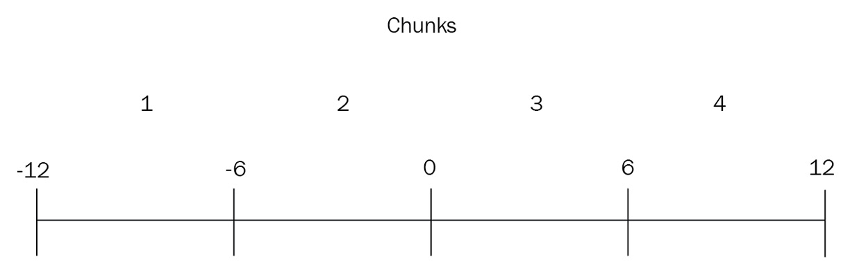
Figure 14.3: Sharding chunks and boundaries

After we insert some data, our chunks will look like this:

• ShardA:
  • Chunk1: -12,-8,-7
  • Chunk2: -6
• ShardB:
  • Chunk3: 0, 2
  • Chunk4: 7, 8, 9, 10, 11, 11, 11, 11

The following diagram illustrates the preceding explanation:

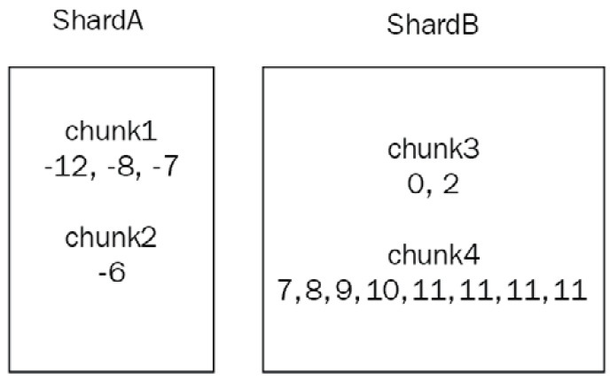
Figure 14.4: Sharding chunks and shard allocation

In this case, we observe that chunk4 has more items than any other chunk. MongoDB will first split chunk4 into two new chunks, attempting to keep the size of each chunk under a certain threshold (128 megabytes (MB) by default, starting from MongoDB 6.0).

Now, instead of chunk4, we have chunk4A: 7, 8, 9, 10 and chunk4B: 11, 11, 11, 11.

The following diagram illustrates the preceding explanation:

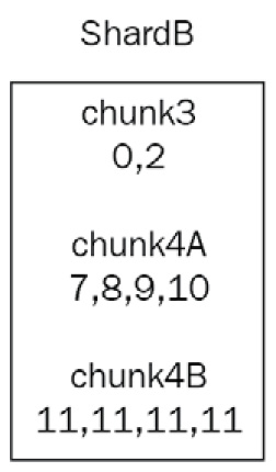
Figure 14.5: Sharding chunks and shard allocation (continued)

The new bounds of this are provided here:

• chunk4A: [6,11)
• chunk4B: [11,12)

Note that chunk4B can only hold one value. This is now an indivisible chunk—a chunk that cannot be broken down into smaller ones anymore—and will grow in size unbounded, causing potential performance issues down the line.

This clarifies why we need to use a high-cardinality field as our shard key and why something such as a Boolean, which only has true/false values, is a bad choice for a shard key.

In our case, we now have two chunks in ShardA and three chunks in ShardB. Let’s look at the following table:

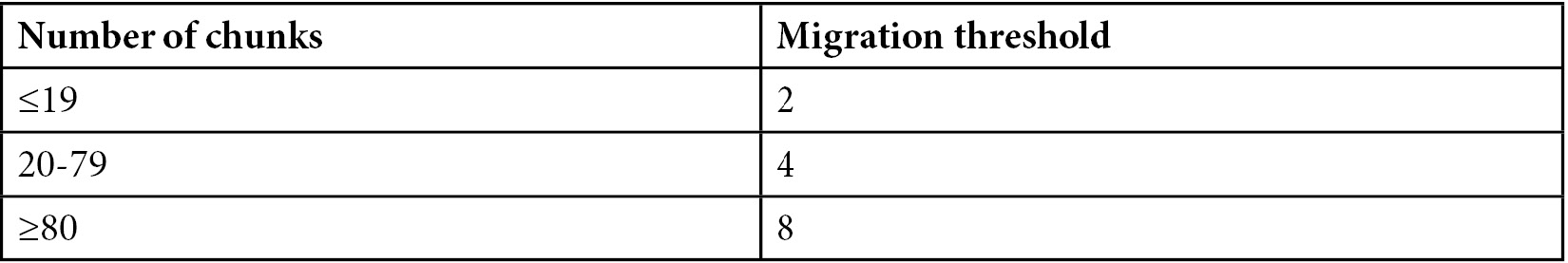
Table 14.1: Sharding number of chunks in each shard and migration threshold

We have not reached our migration threshold yet, since 3-2 = 1.

The migration threshold is calculated as the number of chunks in the shard with the highest count of chunks and the number of chunks in the shard with the lowest count of chunks, as follows:

• Shard1 -> 85 chunks
• Shard2 -> 86 chunks
• Shard3 -> 92 chunks

In the preceding example, balancing will not occur until Shard3 (or Shard2) reaches 93 chunks because the migration threshold is 8 for ≥80 chunks, and the difference between Shard1 and Shard3 is still 7 chunks (92-85).

If we continue adding data in chunk4A, it will eventually be split into chunk4A1 and chunk4A2.

We now have four chunks in ShardB (chunk3, chunk4A1, chunk4A2, and chunk4B) and two chunks in ShardA (chunk1 and chunk2).

The following diagram illustrates the relationships of the chunks to the shards:

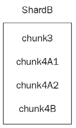
Figure 14.6: Sharding chunks and shards

The MongoDB balancer will now migrate one chunk from ShardB to ShardA as 4-2 = 2, reaching the migration threshold for fewer than 20 chunks. The balancer will adjust the boundaries between the two shards in order to be able to query more effectively (targeted queries). The following diagram illustrates the preceding explanation:

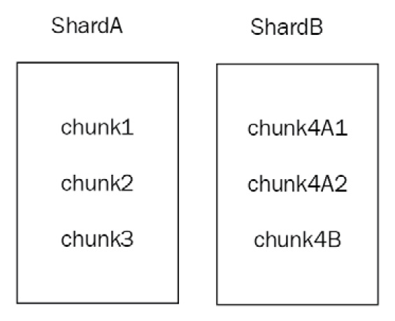
Figure 14.7: Sharding chunks and shards (continued)

As you can see from the preceding diagram, MongoDB will try to split >128 MB chunks in half in terms of size. The bounds between the two resulting chunks may be completely uneven if our data distribution is uneven to begin with. MongoDB can split chunks into smaller ones but cannot merge them automatically. We need to manually merge chunks—a delicate and operationally expensive procedure.

Chunk administration

Most of the time, we should leave chunk administration to MongoDB. We should manually manage chunks at the start, upon receiving the initial load of data, when we change our configuration from a replica set to sharding.

Global shard read/write concern

We can set the read and write concern in a replica-set level via the primary server’s mongod server.We can set the read and write concern in a sharded cluster level via the mongos server.

We need to run the following command while connected to the admin database:

db.adminCommand(

  {

    setDefaultRWConcern : 1,

    defaultReadConcern: { <read concern> },

    defaultWriteConcern: { <write concern> },

    writeConcern: { <write concern> },

    comment: <any>

  }

)

This contains the following parameters:

• setDefaultRWConcern must be set to 1 (true).
• Either defaultReadConcern or defaultWriteConcern or both of these parameters need to be set.
• The defaultReadConcern parameter for the read concern can only be one of the local, available, or majority levels.
• The defaultWriteConcern parameter for the write concern can be any w value greater than 0. This means that at least one server needs to acknowledge the write.
• The writeConcern parameter is the write concern to use for this command.
• comment is an optional description that will appear in logs and other mongo auditing storage.

Moving chunks

To move a chunk manually, we need to issue the following command after connecting to mongos and the admin database:

> db.runCommand( { moveChunk : 'mongo_books.books' ,

find : {id: 50},

to : 'shard1.packtdb.com' } )

Using the preceding command, we move the chunk containing the document with id: 50 (this has to be the shard key) from the books collection of the mongo_books database to the new shard named shard1.packtdb.com.

We can also more explicitly define the bounds of the chunk that we want to move. Now, the syntax looks like this:

> db.runCommand( { moveChunk : 'mongo_books.books' ,

bounds :[ { id : <minValue> } ,

{ id : <maxValue> } ],

to : 'shard1.packtdb.com' } )

Here, minValue and maxValue are the values that we get from db.printShardingStatus().

In the example used previously, for chunk2, minValue would be -6 and maxValue would be 0.

Note

Do not use find in hash-based sharding. Use bounds instead.

Changing the default chunk size

To change the default chunk size, we need to connect to a mongos router and—consequently—to the config database.

Then, we issue the following command to change our global chunksize value to 16 MB:

> db.settings.save( { _id:"chunksize", value: 16 } )

The main reasoning behind changing chunksize comes from cases where the default chunksize value of 128 MB can cause more I/O than our hardware can handle. In this case, defining a smaller chunksize value will result in more frequent but less data-intensive migrations.

Changing the default chunk size has the following drawbacks:

• Creating more splits by defining a smaller chunk size cannot be undone automatically.
• Increasing the chunk size will not force any chunk migration; instead, chunks will grow through inserts and updates until they reach the new size.
• Lowering the chunk size may take quite some time to complete.
• Automatic splitting to comply with the new chunk size if it is lower will only happen upon an insert or update operation. We may have chunks that don’t get any write operations and thus will not be changed in size.

The chunk size can be from 1 to 1,024 MB.

Jumbo chunks

In rare cases, we may end up with jumbo chunks—chunks that are larger than the chunk size and cannot be split by MongoDB. We may also run into the same situation if the number of documents in our chunk exceeds the maximum document limit.

These chunks will have the jumbo flag enabled. Ideally, MongoDB will keep track of whether it can split the chunk, and, as soon as it can, it will get split; however, we may decide that we want to manually trigger a split before MongoDB does.

The way to do this is set out in the following steps:

1. Connect via a shell to your mongos router and run the following code:

   > sh.status(true)

2. Identify the chunk that has jumbo in its description using the following code:

   databases:

   …

   mongo_books.books

   ...

   chunks:

   …

   shardB 2

   shardA 2

   { "id" : 7 } -->> { "id" : 9 } on : shardA Timestamp(2, 2) jumbo

3. Invoke splitAt() or splitFind() manually to split the chunk on the books collection of the mongo_books database at the id value that is equal to 8 using the following code:

   > sh.splitAt( "mongo_books.books", { id: 8 })

Note

The splitAt() function will split based on the split point we define. The two new splits may or may not be balanced.

Alternatively, if we want to leave it to MongoDB to find where to split our chunk, we can use splitFind, as follows:

> sh.splitFind("mongo_books.books", {id: 7})

The splitFind phrase will try to find the chunk that the id:7 query belongs to and automatically define new bounds for the split chunks so that they are roughly balanced.

In both cases, MongoDB will try to split the chunk, and if successful, it will remove the jumbo flag from it.

4. If the preceding operation is unsuccessful, then—and only then—should we try stopping the balancer first, while also verifying the output and waiting for any pending migrations to finish first, as shown in the following code snippet:

   > sh.stopBalancer()

   > sh.getBalancerState()

   > use config

   while( sh.isBalancerRunning() ) {

   print("waiting...");

   sleep(1000);

   }

This should return false.

5. Wait for any waiting… messages to stop printing, and then find the jumbo-flagged chunk in the same way as before.
6. Then, update the chunks collection in your config database of the mongos router, like this:

   > db.getSiblingDB("config").chunks.update(

   { ns: "mongo_books.books", min: { id: 7 }, jumbo: true },

   { $unset: { jumbo: "" } }

   )

The preceding command is a regular update() command, with the first argument being the find() part to find out which document to update and the second argument being the operation to apply to it ($unset: jumbo flag).

7. After all this is done, we re-enable the balancer, as follows:

   > sh.setBalancerState(true)

8. Then, we connect to the admin database to flush the new configuration to all nodes, as follows:

   > db.adminCommand({ flushRouterConfig: 1 } )

Note

Always back up the config database before modifying any state manually.

Merging chunks

As we have seen previously, MongoDB will usually adjust the bounds for each chunk in our shard to make sure that our data is equally distributed. This may not work in some cases—especially when we define chunks manually—if our data distribution is surprisingly unbalanced, or if we have many delete operations in our shard.

Having empty chunks will invoke unnecessary chunk migrations and give MongoDB a false impression of which chunk needs to be migrated. As we have explained before, the threshold for chunk migration is dependent on the number of chunks that each shard holds. Having empty chunks may or may not trigger the balancer when it’s needed.

Chunk merging can only happen when at least one of the chunks is empty, and only between adjacent chunks.

To find empty chunks, we need to connect to the database that we want to inspect (in our case, mongo_books) and use runCommand with dataSize set, as follows:

> use mongo_books

> db.runCommand({

 "dataSize": "mongo_books.books",

 "keyPattern": { id: 1 },

 "min": { "id": -6 },

 "max": { "id": 0 }

})

The dataSize phrase follows the database_name.collection_name pattern, whereas keyPattern is the shard key that we have defined for this collection.

The min and max values should be calculated by the chunks that we have in this collection. In our case, we have entered chunkB’s details from the example earlier in this chapter.

If the bounds of our query (which, in our case, are the bounds of chunkB) return no documents, the result will resemble the following:

{ "size" : 0, "numObjects" : 0, "millis" : 0, "ok" : 1 }

Now that we know that chunkB has no data, we can merge it with another chunk (in our case, this could only be chunkA), like so:

> db.runCommand( { mergeChunks: "mongo_books.books",

 bounds: [ { "id": -12 },

 { id: 0 } ]

 } )

Upon success, this will return MongoDB’s default ok status message, as shown in the following code snippet:

{ "ok" : 1 }

We can then verify that we only have one chunk on ShardA by invoking sh.status() again.

Adding and removing shards

Adding a new shard to our cluster is as easy as connecting to mongos, connecting to the admin database, and invoking runCommand with the following code:

> db.runCommand( {

addShard: "mongo_books_replica_set/rs01.packtdb.com:27017", maxSize: 18000, name: "packt_mongo_shard_UK"

} )

This adds a new shard from the replica set named mongo_books_replica_set from the rs01.packtdb.com host running on port 27017. We also define the maxSize value of data for this shard as 18000 MB (or we can set it to 0 to give it no limit) and the name of the new shard as packt_mongo_shard_UK.

Note

This operation will take quite some time to complete as chunks will have to be rebalanced and migrated to the new shard.

Removing a shard, on the other hand, requires more involvement since we have to make sure that we won’t lose any data on the way. We do this like so:

1. First, we need to make sure that the balancer is enabled using sh.getBalancerState(). Then, after identifying the shard we want to remove using any one of the sh.status(), db.printShardingStatus(), or listShards admin commands, we connect to the admin database and invoke removeShard, as follows:

   > use admin

   > db.runCommand( { removeShard: "packt_mongo_shard_UK" } )

The output should contain the following elements:

...

"msg" : "draining started successfully",

"state" : "started",

...

2. Then, if we invoke the same command again, we get the following output:

   > db.runCommand( { removeShard: "packt_mongo_shard_UK" } )

   …

   "msg" : "draining ongoing",

   "state" : "ongoing",

   "remaining" : {

   "chunks" : NumberLong(2),

   "dbs" : NumberLong(3)

   },

   …

The remaining document in the result contains the number of chunks and dbs instances that are still being transferred. In our case, it’s 2 and 3 respectively.

Note

All the commands need to be executed in the admin database.

An extra complication in removing a shard can arise if the shard we want to remove serves as the primary shard for one or more of the databases that it contains. The primary shard is allocated by MongoDB when we initiate sharding, so when we remove the shard, we need to manually move these databases to a new shard.

3. We will know whether we need to perform this operation by looking at the following section of the result from removeShard():

   ...

   "note" : "you need to drop or movePrimary these databases",

   "dbsToMove" : [

   "mongo_books"

   ],

   ...

We need to drop or perform movePrimary on our mongo_books database. The way to do this is to first make sure that we are connected to the admin database.

Note

We need to wait for all of the chunks to finish migrating before running the previous command.

4. Make sure that the result contains the following elements before proceeding:

   ..."remaining" : {

   "chunks" : NumberLong(0) }...

5. Only after we have made sure that the chunks to be moved are down to zero can we safely run the following command:

   > db.runCommand( { movePrimary: "mongo_books", to: "packt_mongo_shard_EU" })

6. This command will invoke a blocking operation, and when it returns, it should have the following result:

   { "primary" : "packt_mongo_shard_EU", "ok" : 1 }

7. Invoking the same removeShard() command after we are all done should return the following result:

   > db.runCommand( { removeShard: "packt_mongo_shard_UK" } )

   ... "msg" : "removeshard completed successfully",

   "state" : "completed",

   "shard" : "packt_mongo_shard_UK"

   "ok" : 1

   ...

8. Once we get to state as completed and ok as 1, it is safe to remove our packt_mongo_shard_UK shard.

Removing a shard is naturally more complicated than adding one. We need to allow some time, hope for the best, and plan for the worst when performing potentially destructive operations on our live cluster.

Sharding limitations

Sharding comes with great flexibility. Unfortunately, there are a few limitations in the way that we perform some of the operations.

We will highlight the most important ones in the following list:

• The group() database command does not work. The group() command should not be used anyway; use aggregate() and the aggregation framework instead, or mapreduce().
• The db.eval() command does not work and should be disabled in most cases for security reasons.
• The $isolated option for updates does not work. This is a functionality that is missing in sharded environments. The $isolated option for update() provides the guarantee that, if we update multiple documents at once, other readers and writers will not see some of the documents updated with the new value, and the others will still have the old value. The way this is implemented in unsharded environments is by holding a global write lock and/or serializing operations to a single thread to make sure that every request for the documents affected by update() will not be accessed by other threads/operations. This implementation means that it is not performant and does not support any concurrency, which makes it prohibitive to allow the $isolated operator in a sharded environment.
• The $snapshot operator for queries is not supported. The $snapshot operator in the find() cursor prevents documents from appearing more than once in the results, as a result of being moved to a different location on the disk after an update. The $snapshot operator is operationally expensive and often not a hard requirement. The way to substitute it is by using an index for our queries on a field whose keys will not change for the duration of the query.
• The indexes cannot cover our queries if our queries do not contain the shard key. Results in sharded environments will come from the disk and not exclusively from the index. The only exception is if we query only on the built-in _id field and return only the _id value, in which case, MongoDB can still cover the query using built-in indexes.
• update() and remove() operations work differently. All update() and remove() operations in a sharded environment must include either the _id field of the documents that are to be affected or the shard key; otherwise, the mongos router will have to do a full table scan across all collections, databases, and shards, which would be operationally very expensive.
• Unique indexes across shards need to contain the shard key as a prefix of the index. In other words, to achieve the uniqueness of documents across shards, we need to follow the data distribution that MongoDB follows for the shards.
• The shard key has to be up to 512 bytes in size. The shard key index has to be in ascending order on the key field that gets sharded and—optionally—other fields as well, or a hashed index on it.

After discussing sharding administration, monitoring, and its limitations, we will move on to learn how it can be different querying data stored in a sharded cluster as opposed to a single-server or a single-replica-set architecture.

Querying sharded data

Querying our data using a MongoDB shard is different than a single-server deployment or a replica set. Instead of connecting to the single server or the primary of the replica set, we connect to the mongos router, which decides which shard to ask for our data. In this section, we will explore how the query router operates and use Ruby to illustrate how similar to a replica set this is for the developer.

The query router

The query router, also known as the mongos process, acts as the interface and entry point to our MongoDB cluster. Applications connect to it instead of connecting to the underlying shards and replica sets; mongos executes queries, gathers results, and passes them to our application.

The mongos process doesn’t hold any persistent state and is typically low on system resources. It acts as a proxy for requests. When a query comes in, mongos will examine it, decide which shards need to execute the query, and establish a cursor in each one of them.

Note

The mongos process is typically hosted in the same instance as the application server.

find

If our query includes the shard key or a prefix of the shard key, mongos will perform a targeted operation, only querying the shards that hold the keys we are looking for.

For example, with a composite shard key of {_id, email, address} on our User collection, we can have a targeted operation with any of the following queries:

> db.User.find({_id: 1})

> db.User.find({_id: 1, email: '[email protected]'})

> db.User.find({_id: 1, email: '[email protected]', address: 'Linwood Dunn'})

These queries consist of either a prefix (as is the case with the first two) or the complete shard key.

On the other hand, a query on {email, address} or {address} will not be able to target the right shards, resulting in a broadcast operation. A broadcast operation is any operation that doesn’t include the shard key or a prefix of the shard key, and they result in mongos querying every shard and gathering results from them. They are also known as scatter-and-gather operations or fan-out queries.

Note

This behavior is a direct result of the way indexes are organized and is similar to the behavior that we identified in the chapter about indexing.

Query results may be affected by transaction writes. For example, if we have multiple shards and a transaction writes document A in shard A, which is committed, and document B in shard B, which is not yet committed, querying with read concern local in shard A will return document A, ignoring document B in shard B. Because of the read concern “local”, MongoDB will not reach out into shard B to retrieve document B.

sort/limit/skip

If we want to sort our results, we have the following two options:

• If we are using the shard key in our sort criteria, then mongos can determine the order in which it has to query a shard or shards. This results in an efficient and, again, targeted operation.
• If we are not using the shard key in our sort criteria, then—as is the case with a query without any sort criteria—it’s going to be a fan-out query. To sort the results when we are not using the shard key, the primary shard executes a distributed merge sort locally before passing on the sorted result set to mongos.

A limit on the queries is enforced on each individual shard and then again at the mongos level, as there may be results from multiple shards. A skip operator, on the other hand, cannot be passed on to individual shards and will be applied by mongos after retrieving all the results locally.

If we combine the skip and limit operators, mongos will optimize the query by passing both values to individual shards. This is particularly useful in cases such as pagination. If we query without sort and the results are coming from more than one shard, mongos will round-robin across shards for the results.

update/remove

In document modifier operations, such as update and remove, we have a similar situation to the one we saw with find. If we have the shard key in the find section of the modifier, then mongos can direct the query to the relevant shard.

If we don’t have the shard key in the find section, then it will again be a fan-out operation.

Note

UpdateOne, replaceOne, and removeOne operations must have the shard key or the _id value.

The following table sums up the operations that we can use with sharding:

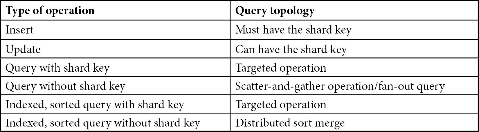
Table 14.2: Sharding and create, read, update, and delete (CRUD) operations

Hedged reads

If we use non-primary read preference and MongoDB v>=4.4, then the MongoDB router (mongos) will by default attempt to hedge reads—for example, when we invoke find(). For each operation, it will send the request to two members for each shard (replica set). Whichever request returns first will be the return value, and the other request will either return and be discarded or time out after maxTimeMSForHedgedReads milliseconds (msecs)—the default is 150.

Querying using Ruby

Connecting to a sharded cluster using Ruby or any other language is no different than connecting to a replica set. Using the official Ruby driver, we have to configure the client object to define a set of mongos servers, as shown in the following code snippet:

client = Mongo::Client.new('mongodb://key:password@mongos-server1-host:mongos-server1-port,mongos-server2-host:mongos-server2-port/admin?ssl=true&authSource=admin')

mongo-ruby-driver will then return a client object, which is no different than connecting to a replica set from the Mongo Ruby client. We can then use the client object as we did in previous chapters, with all the caveats around how sharding behaves differently from a standalone server or a replica set with regard to querying and performance.

Performance comparison with replica sets

Developers and architects are always looking out for ways to compare performance between replica sets and sharded configurations.

The way MongoDB implements sharding is based on top of replica sets. Every shard in production should be a replica set. The main difference in performance comes from fan-out queries. When we are querying without the shard key, MongoDB’s execution time is limited by the worst-performing replica set. In addition, when using sorting without the shard key, the primary server has to implement the distributed merge sort on the entire dataset. This means that it has to collect all data from different shards, merge sort them, and pass them as sorted to mongos. In both cases, network latency and limitations in bandwidth can slow down operations, which they wouldn’t do with a replica set.

On the flip side, by having three shards, we can distribute our working-set requirements across different nodes, thereby serving results from RAM instead of reaching out to the underlying storage—HDD or SSD.

On the other hand, writes can be sped up significantly since we are no longer bound by a single node’s I/O capacity, and we can have writes in as many nodes as there are shards. Summing up, in most cases—and especially for cases where we are using the shard key—both queries and modification operations will be significantly sped up by sharding.

Note

The shard key is the single most important decision in sharding and should reflect and apply to our most common application use cases.

Querying a sharded cluster needs some extra consideration from the application developer’s perspective. In the next section, we will learn how to recover from operational issues.

Sharding recovery

In this section, we will explore different failure types and how we can recover in a sharded environment. Failure in a distributed system can take multiple forms and shapes. In this section, we will cover all possible failure cases, as outlined here:

• A mongos process breaks
• A mongod process breaks
• A config server breaks
• A shard goes down
• The entire cluster goes down

In the following sections, we will describe how each component failure affects our cluster and how to recover.

mongos

The mongos process is a relatively lightweight process that holds no state. In the case that the process fails, we can just restart it or spin up a new process on a different server. It’s recommended that mongos processes are located in the same server as our application, and so it makes sense to connect from our application using the set of mongos servers that we have colocated in our application servers to ensure high availability (HA) of mongos processes.

mongod

A mongod process failing in a sharded environment is no different than it failing in a replica set. If it is a secondary, the primary and the other secondary (assuming three-node replica sets) will continue as usual.

If it is a mongod process acting as a primary, then an election round will start to elect a new primary in this shard (which is really a replica set).

In both cases, we should actively monitor and try to repair the node as soon as possible, as our availability can be impacted.

Config server

Config servers must be configured as a replica set. A config server failing is no different than a regular mongod process failing. We should monitor, log, and repair the process.

A shard goes down

Losing an entire shard is pretty rare, and in many cases can be attributed to network partitioning rather than failing processes. When a shard goes down, all operations that would go to this shard will fail. We can (and should) implement fault tolerance at our application level, allowing our application to resume for operations that can be completed.

Choosing a shard key that can easily map on our operational side can also help; for example, if our shard key is based on location, we may lose the European Union (EU) shard, but will still be able to write and read data regarding United States (US)-based customers through our US shard.

The entire cluster goes down

If we lose the entire cluster, we can’t do anything other than get it back up and running as soon as possible. It’s important to have monitoring and to put a proper process in place to understand what needs to be done, when, and by whom, should this ever happen.

Recovering when the entire cluster goes down essentially involves restoring from backups and setting up new shards, which is complicated and will take time. Dry testing this in a staging environment is also advisable, as is investing in regular backups via MongoDB Ops Manager or any other backup solution.

Note

A member of each shard’s replica set could be in a different location for disaster-recovery (DR) purposes.

Further reading

The following sources are recommended for you to study sharding in depth:

• Scaling MongoDB by Kristina Chodorow
• MongoDB: The Definitive Guide by Kristina Chodorow and Michael Dirolf
• MongoDB manual—Sharding: https://docs.mongodb.com/manual/sharding/
• MongoDB sharding pitfalls: https://www.mongodb.com/blog/post/sharding-pitfalls-part-iii-chunk-balancing-and
• MongoDB sharding and chunks: http://plusnconsulting.com/post/mongodb-sharding-and-chunks/
• MongoDB sharding internals: https://github.com/mongodb/mongo/wiki/Sharding-Internals
• MongoDB sharding: http://learnmongodbthehardway.com/schema/sharding
• MongoDB sharding and replica sets release (v1.6): https://www.infoq.com/news/2010/08/MongoDB-1.6
• Horizontal and vertical scaling explained: http://www.pc-freak.net/images/horizontal-vs-vertical-scaling-vertical-and-horizontal-scaling-explained-diagram.png

Summary

In this chapter, we explored sharding, one of the most interesting features of MongoDB. We started with an architectural overview of sharding and moved on to how we can design a shard and choose the right shard key.

We learned about monitoring, administration, and the limitations that come with sharding. We also learned about mongos, the MongoDB sharding router that directs our queries to the correct shard. Finally, we discussed recovery from common failure types in a MongoDB sharded environment.

The next chapter, on fault tolerance and high availability, will offer some useful tips and tricks that have not been covered in the other chapters.