17

Multi-Step Forecasting

In the previous parts, we covered some basics of forecasting and different types of modeling techniques for time series forecasting. But a complete forecasting system is not just the model. There are a few mechanics of time series forecasting that make a lot of difference. These topics cannot be called basics because they require a nuanced understanding of the forecasting paradigm, and that is why we didn’t cover these upfront.

Now that you have worked on some forecasting models and are familiar with time series, it’s time to get more nuanced in our approach. Most of the forecasting exercises we have done throughout the book focus on forecasting the next timestep.

In this chapter, we will look at strategies to generate multi-step forecasting. In other words, how to forecast the next timesteps.

In this chapter, we will be covering these main topics:

• Why multi-step forecasting?
• Recursive strategy
• Direct strategy
• Joint strategy
• Hybrid strategies
• How to choose a multi-step forecasting strategy

Why multi-step forecasting?

A multi-step forecasting task consists of forecasting the next timesteps, , of a time series, , where . Most real-world applications of time series forecasting demand multi-step forecasting, whether it is the energy consumption of a household or the sales of a product. This is because forecasts are never created to know what will happen in the future, but to take some action using the visibility we get. To effectively take any action, we would want to know the forecast a little ahead of time. For instance, the dataset we have been using throughout the book is about the energy consumption of households, logged every half an hour. If the energy provider wants to plan its energy production to meet customer demand, the next half an hour doesn’t help at all. Similarly, if we look at the retail scenario, where we want to forecast the sales of a product, we will want to forecast a few days ahead so that we can purchase necessary goods, ship them to the store, and so on, in time for the demand.

Despite a more prevalent use case, multi-step forecasting has not received the attention it deserves. One of the reasons for that is the existence of classical statistical models or econometrics models such as the ARIMA and exponential smoothing methods, which include the multi-step strategy bundled within what we call a model; because of that, these models can generate multiple timesteps without breaking a sweat (although, as we will see in the chapter, they rely on one specific multi-step strategy to generate their forecast). Because these models were the most popular models used, practitioners need not have worried about multi-step forecasting strategies. But the advent of machine learning (ML) and deep learning (DL) methods for time series forecasting has opened up the need for a more focused study of multi-step forecasting strategies once again.

Another reason for the lower popularity of multi-step forecasting is that it is simply harder than single-step forecasting. This is because the more steps we extrapolate into the future, the more uncertainty in the predictions due to complex interactions between the different steps ahead.

There are many strategies that can be used to generate multi-step forecasting, and the following figure summarizes them neatly:

Figure 17.1 – Multi-step forecasting strategies

Each node of the graph in Figure 17.1 is a strategy, and different strategies that have common elements have been linked together with edges in the graph. In the rest of the chapter, we will be covering each of these nodes (strategies) and explaining them in detail.

Let’s establish a few basic notations to help us understand these strategies. We have a time series, , of timesteps, . denotes the same series, but ending at timestep . We also consider a function, , which generates a window of size from a time series. This function is a proxy for how we prepare the inputs for the different models we have seen throughout the book. So, if we see , it means the function would draw a window from that ends at timestep . We will also consider to be the forecast horizon, where . We will also be using as an operator, which denotes concatenation.

Now, let’s look at the different strategies (#1 in References is a good survey paper for different strategies). The discussion about merits and where we can use each of them is bundled in another upcoming section.

Recursive strategy

The recursive strategy is the oldest, most intuitive, and most popular technique to generate multi-step forecasts. To understand a strategy, there are two major regimes we have to understand:

• How is the training of the models done?
• How are the trained models used to generate forecasts?

Let’s take the help of a diagram to understand the recursive strategy:

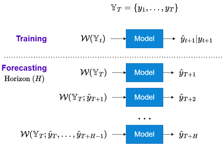
Figure 17.2 – Recursive strategy for multi-step forecasting

Let’s discuss these regimes in detail.

Training regime

The recursive strategy involves training a single model to perform a one-step-ahead forecast. We can see in Figure 17.1 that we use the window function, , to draw a window from and train the model to predict . And during training, a loss function (which measures the divergence between the output of the model, , and the actual value, ) is used to optimize the parameters of the model.

Forecasting regime

We have trained a model to do one-step-ahead predictions. Now, we use this model in a recursive fashion to generate forecasts timesteps ahead. For the first step, we use , the window using the latest timestamp in training data, and generate the forecast one step ahead, . Now, this generated forecast is added to the history and a new window is drawn from this history, . This window is given as the input to the same one-step-ahead model, and the forecast for the next timestep, , is generated. This process is repeated until we get forecasts for all timesteps.

This is the strategy that classical models that have stood the test of time (such as ARIMA and Exponential Smoothing) use internally when they generate multi-step forecasts. In the ML context, this means that we will train a model to predict one step ahead (as we have done all through this book), and then do a recursive operation where we forecast one step ahead, use the new forecast to recalculate all the features such as lags, rolling windows, and so on, and forecast the next step. In the context of the DL models, we can think of this as adding the forecast into the context window and using the trained model to generate the next step.

Direct strategy

The direct strategy, also called the independent strategy, is a popular strategy in forecasting using ML. This involves forecasting each horizon independently of each other. Let’s look at the diagram first:

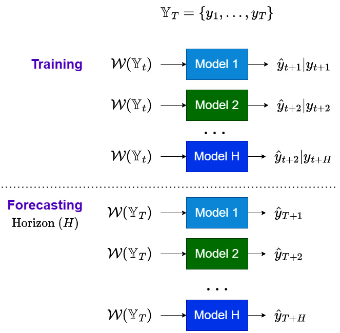
Figure 17.3 – Direct strategy for multi-step forecasting

Next, let’s discuss the regimes in detail.

Training regime

Under the direct strategy, we train different models, which take in the same window function but are trained to predict different timesteps in the forecast horizon. Therefore, we are learning a separate set of parameters, one for each timestep in the horizon, such that all the models combined learn a direct and independent mapping from the window, , to the forecast horizon, .

This strategy has gained ground along with the popularity of ML-based time series forecasting. From the ML context, we can practically implement it in two ways:

• Shifting targets – Each model in the horizon is trained by shifting the target by that many steps as the horizon we are training the model to forecast.
• Eliminating features – Each model in the horizon is trained by using only the features that are allowable to use according to the rules. For instance, when predicting , we can’t use lag 1 (because to predict , we will not have actuals for ).

Important note

The two ways mentioned in the preceding list work nicely if we only have lags as features. For instance, for eliminating features, we can just drop the offending lags and train the model. But in cases where we are using rolling features and other more sophisticated features, simple dropping doesn’t work because lag 1 is already used in calculating the rolling features. This leads to data leakage. In such scenarios, we can make a dynamic function that calculates these features taking in a parameter to specify the horizon we are creating these features for. All the helper methods we used in Chapter 6, Feature Engineering for Time Series Forecasting, (add_rolling_features, add_seasonal_rolling_features, and add_ewma) have a parameter called n_shift, which handles this condition. If we are training a model for , we need to pass n_shift=2 and the method will take care of the rest. Now, while training the models, we use this dynamic method to recalculate these features for each horizon separately.

Forecasting regime

The forecasting regime is also fairly straightforward. We have the H trained models, one for each timestep in the horizon, and we use to forecast each of them independently.

Joint strategy

The previous two strategies consider the model to have a single output. This is the case with most ML models; we formulate the model to predict a single scalar value as the prediction after taking in an array of inputs: multiple input, single output (MISO). But there are some models, such as the DL models, which can be configured to give us multiple outputs. Therefore, the joint strategy, also called multiple input, multiple output (MIMO), aims to learn a single model that produces the entire forecasting horizon as an output:

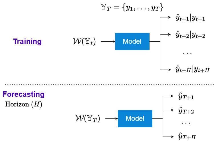
Figure 17.4 – Joint strategy for multi-step forecasting

Let’s see how these regimes work.

Training regime

The joint strategy involves training a single multi-output model to forecast all the timesteps in the horizon at once. We can see in Figure 17.1 that we use the window function, , to draw a window from and train the model to predict . And during training, a loss function that measures the divergence between all the outputs of the model, , and the actual values, , is used to optimize the parameters of the model.

Forecasting regime

The forecasting regime is also very simple. We have a trained model that is able to forecast all the timesteps in the horizon and we use to forecast them at once.

This strategy is typically used in DL models where we configure the last layer to output scalars instead of 1.

We have already seen this strategy in action at multiple places in the book:

• The Tabular Regression (Chapter 13, Common Modeling Patterns for Time Series) paradigm can easily be extended to output the whole horizon.
• We have seen Sequence-to-Sequence models with a fully connected decoder (Chapter 13, Common Modeling Patterns for Time Series) using this strategy for multi-step forecasting.
• In Chapter 14, Attention and Transformers for Time Series, we used this strategy to forecast using transformers.
• In Chapter 16, Specialized Deep Learning Architectures for Forecasting, we saw models such as N-BEATS, N-HiTS, and Temporal Fusion Transformer, which used this strategy to generate multi-step forecasts.

Hybrid strategies

The three strategies we have already covered are the three basic strategies for multi-step forecasting, each with its own merits and demerits. Over the years, researchers have tried to combine these into hybrid strategies that try to capture the good parts of all these strategies. Let’s go through a few of them here. This will not be a comprehensive list because there is none. Anyone with enough creativity can come up with alternate strategies, but we will just cover a few that have received some attention and deep study from the forecasting community.

DirRec Strategy

As the name suggests, the DirRec strategy is the combination of direct and recursive strategies for multi-step forecasting. First, let’s look at the following diagram:

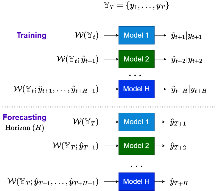
Figure 17.5 – DirRec strategy for multi-step forecasting

Now, let’s see how these regimes work for the DirRec strategy.

Training regime

Similar to the direct strategy, the DirRec strategy also has models for a forecasting horizon of , but with a twist. We start the process by using and train a model to predict one step ahead. In the recursive strategy, we used this forecasted timestep in the same model to predict the next timestep. But in DirRec, we train a separate model for , but using the forecast we generated in . To generalize at timestep , in addition to , we include all the forecasts generated by different models at timesteps to .

Forecasting regime

The forecasting regime is just like the training regime, but instead of training the models, we use the trained models to generate the forecasts in a recursive manner.

Iterative block-wise direct strategy

The iterative block-wise direct (IBD) strategy is also called the iterative multi-SVR strategy, paying homage to the research paper that suggested this (#2 in References). The direct strategy requires different models to train, and that makes it difficult to scale for long-horizon forecasting. The IBD strategy tries to tackle that shortcoming by using a block-wise iterative style of forecasting:

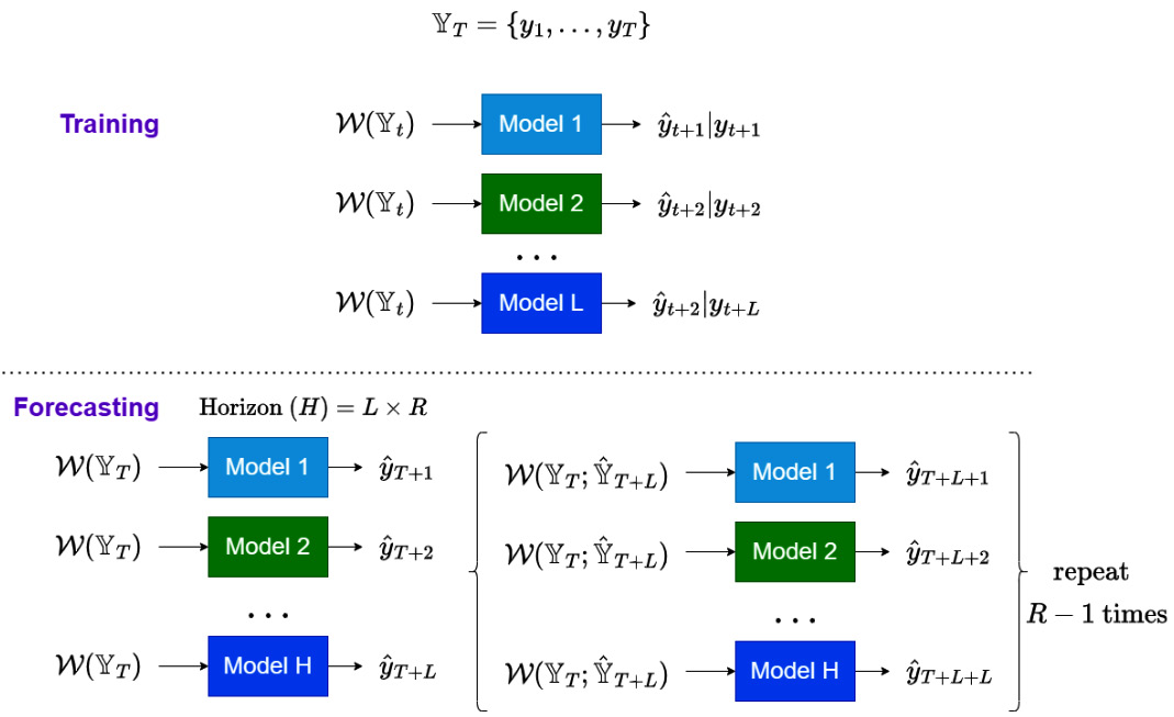
Figure 17.6 – IBD strategy for multi-step forecasting

Let’s understand the training and forecasting regimes for this strategy.

Training regime

In the IBD strategy, we split the forecast horizon, , into blocks of length , such that . And instead of training direct models, we train direct models.

Forecasting regime

While forecasting, we use the trained models to generate the forecast for the first timesteps ( to ) in using the window . Let’s denote this L forecast as . Now, we will use , along with , in the window function to draw a new window, . This new window is used to generate the forecast for the next timesteps ( to ). This process is repeated many times to complete the full horizon forecast.

Rectify strategy

The rectify strategy is another way we can combine direct and recursive strategies. It strikes a middle ground between the two by forming a two-stage training and inferencing methodology. We can see this as a model stacking approach (Chapter 9, Ensembling and Stacking) but between different multi-step forecasting strategies:

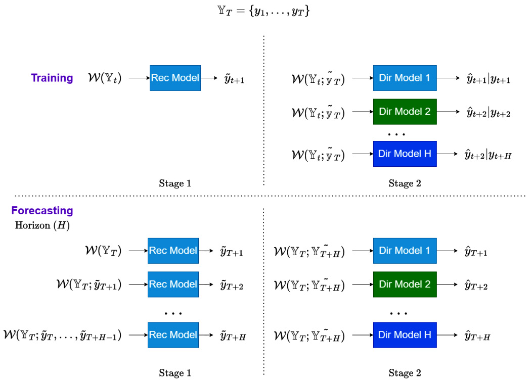
Figure 17.7 – Rectify strategy for multi-step forecasting

Let’s understand how this strategy works.

Training regime

The training happens in two steps. The recursive strategy is applied to the horizon and the forecast for all H timesteps is generated. Let’s call this . Now, we train direct models for each horizon using the original history, , and the recursive forecasts, , as inputs.

Forecasting regime

The forecasting regime is similar to the training, where the recursive forecasts are generated first and they, along with the original history, are used to generate the final forecasts.

RecJoint

True to its name, RecJoint is a mashup between the recursive and joint strategies, but applicable for single-output models:

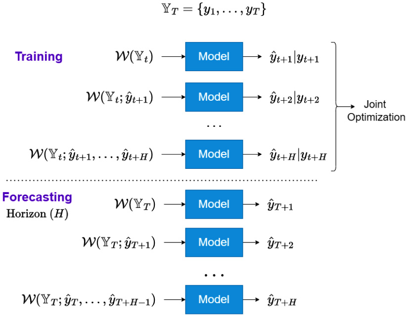
Figure 17.8 – RecJoint strategy for multi-step forecasting

The following sections detail the working of this strategy.

Training regime

The training in the RecJoint strategy is very similar to the recursive strategy in the way it trains a single model and recursively uses prediction at as an input to train , and so on. But the recursive strategy trains the model on just the next timestep. RecJoint generates the predictions for the entire horizon, and jointly optimizes the entire horizon forecasts while training. This forces the model to look at the next H timesteps and jointly optimize the entire horizon instead of the myopic one-step-ahead objective. We saw this strategy at play when we trained Seq2Seq models using an RNN encoder and decoder (Chapter 13, Common Modeling Patterns for Time Series).

Forecasting regime

The forecasting regime for RecJoint is exactly the same as for the recursive strategy.

Now that we have understood a few strategies, let’s also discuss the merits and demerits of these strategies.

How to choose a multi-step forecasting strategy?

Let’s summarize all the different strategies that we learned now in a table:

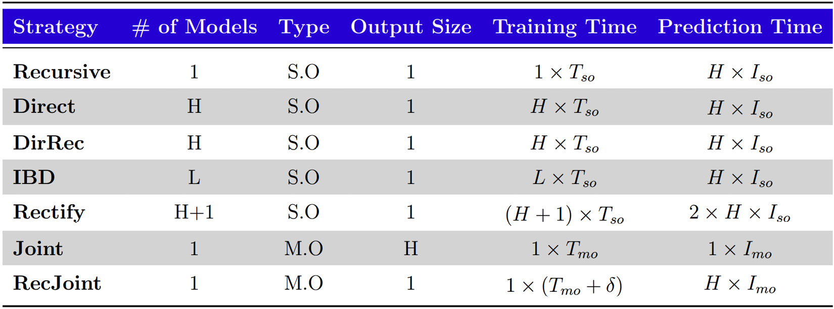
Figure 17.9 – Multi-step forecasting strategies – a summary

Here, the following applies:

• S.O: Single output
• M.O: Multi-output
• and : Training and inferencing time of a single output model
• and : Training and inferencing time of a multi-output model (practically, is larger than mostly because multi-output models are typically DL models and their training time is higher than standard ML models)
• : The horizon
• , where is the number of blocks in the IBD strategy
• is some positive real number

The table will help us understand and decide which strategy is better from multiple perspectives:

• Engineering complexity: Recursive, Joint, RecJoint << IBD << Direct, DirRec << Rectify
• Training time: Recursive << Joint (typically ) << RecJoint << IBD << Direct, DirRec << Rectify
• Inference time: Joint << Direct, Recursive, DirRec, IBD, RecJoint << Rectify

It also helps us to decide the kind of model we can use for each strategy. For instance, a joint strategy can only be implemented with a model that supports multi-output, such as a DL model. But we are yet to discuss how these strategies affect accuracies.

Although in ML, the final word goes to empirical evidence, there are ways we can analyze the different methods to provide us with some guidelines. Taieb et al. analyzed the bias and variance of these multi-step forecasting strategies, both theoretically and using simulated data. With this analysis, along with other empirical findings over the years, we do have an understanding of the strengths and weaknesses of these strategies, and some guidelines from these findings.

Reference check

The research paper by Taieb et al. is cited in References under 3.

Taieb et al. point out several disadvantages of the recursive strategy, contrasting with the direct strategy, based on the bias and variance components of error analysis. They further corroborated these observations through an empirical study as well.

The key points that elucidate the difference in performance are as follows:

• For the recursive strategy, the bias and variance components of error in step affect step . Because of this phenomenon, the errors that a recursive model makes tend to accumulate as we move further in the forecast horizon. But for the direct strategy, this dependence is not explicit and therefore doesn’t suffer the same deterioration that we see in the recursive strategy. This was also seen in the empirical study where the recursive strategy was very erratic and had the highest variance, which increased significantly as we moved further in the horizon.
• For the direct strategy, the bias and variance components of error in step do not affect . This is because each horizon, , is forecasted in isolation. Intuitively, a downside of this approach is the fact that this strategy can produce completely unrelated forecasts across the horizon leading to unrealistic forecasts. The complex dependencies that may exist between the forecast in the horizon are not captured in the direct strategy. For instance, a direct strategy on a time series with a non-linear trend may result in a broken curve because of the independence of each timestep in the horizon.
• Practically, in most cases, a direct strategy produces coherent forecasts.
• The bias for the recursive strategy was also amplified when the forecasting model produces forecasts that have large variations. Highly complex models are known to have low bias but a high amount of variations, and these high variations seem to amplify the bias for recursive strategy models.
• When we have very large datasets, the bias term of the direct strategy becomes zero, but the recursive strategy bias was still non-zero. This was further demonstrated in experiments – for long time series, the direct strategy almost always outperformed the recursive strategy. From the learning theory perspective, we are learning functions using the data for the direct strategy, whereas for recursive, we are just learning . So, with the same amount of data, it is harder to learn true functions than . This is amplified in low-data situations.
• Although the recursive strategy seems inferior to the direct strategy theoretically and empirically, it is not without some advantages:
  • For highly non-linear and noisy time series, learning direct functions for all the horizons can be hard. And in such situations, recursive can work better.
  • If the underlying data-generating process (DGP) is very smooth and can be easily approximated, the recursive strategy can work better.
  • When the time series is shorter, the recursive strategy can work better.
• We talked about the direct strategy generating possible unrelated forecasts for the horizon, but this is exactly the part that the joint strategy takes care of. The joint strategy can be thought of as an extension of the direct strategy, but instead of having different models, we have a single model produce outputs. We are learning a single function instead of H functions from the given data. Therefore, the joint strategy doesn’t have the same weakness as the direct strategy in short time series.
• One of the weaknesses of the joint strategy (and RecJoint) is the high bias on very short horizons (such as , and so on). We are learning a model that optimizes across all the timesteps in the horizon using a standard loss function such as the mean squared error. But these errors are at different scales. The errors that can occur further down the horizon are larger than the ones close by, and this implicitly puts more weight on the longer horizons, and the model learns a function that is skewed toward getting the longer horizons right.
• The joint and RecJoint strategies are comparable from the variance perspective. But the joint strategy can give us a lower bias because the RecJoint strategy learns a recursive function and it may not be flexible enough to capture the pattern. But the joint strategy uses the full power of the forecasting model to directly forecast the horizon.

Hybrid strategies, such as DirRec, IBD, and so on, try to balance the merits and demerits of fundamental strategies such as direct, recursive, and joint. With these merits and demerits, we can make an informed experimentation framework to come up with the best strategy for the problem at hand.

Summary

We touched upon a particular aspect of forecasting that is highly relevant for real-world use cases, but rarely talked about and studied. We saw why we needed multi-step forecasting and then went on to review a few popular strategies we can use. We understood the popular and fundamental strategies such as direct, recursive, and joint, and then went on to look at a few hybrid strategies such as DirRec, rectify, and so on. To top it off, we looked at the merits and demerits of these strategies and discussed a few guidelines for selecting the right strategy for your problem.

In the next chapter, we will be looking at another important aspect of forecasting – evaluation.

References

The following is the list of the references that we used throughout the chapter:

1. Taieb, S.B., Bontempi, G., Atiya, A.F., and Sorjamaa, A. (2012). A review and comparison of strategies for multi-step ahead time series forecasting based on the NN5 forecasting competition. Expert Syst. Appl., 39, 7067-7083: https://arxiv.org/pdf/1108.3259.pdf
2. Li Zhang, Wei-Da Zhou, Pei-Chann Chang, Ji-Wen Yang, Fan-Zhang Li. (2013). Iterated time series prediction with multiple support vector regression models. Neurocomputing, Volume 99, 2013: https://www.sciencedirect.com/science/article/pii/S0925231212005863
3. Taieb, S.B. and Atiya, A.F. (2016). A Bias and Variance Analysis for Multistep-Ahead Time Series Forecasting. in IEEE Transactions on Neural Networks and Learning Systems, vol. 27, no. 1, pp. 62-76, Jan. 2016: https://ieeexplore.ieee.org/document/7064712