2

Acquiring and Processing Time Series Data

In the previous chapter, we learned what a time series is and established a few standard notations and terminologies. Now, let’s switch tracks from theory to practice. In this chapter, we are going to get our hands dirty and start working with data. Although we said time series data is everywhere, we are still yet to get our hands dirty with a few time series datasets. We are going to start working on the dataset we have chosen to work on throughout this book, process it in the right way, and learn about a few techniques for dealing with missing values.

In this chapter, we will cover the following topics:

• Understanding the time series dataset
• pandas datetime operations, indexing, and slicing – a refresher
• Handling missing data
• Mapping additional information
• Saving and loading files to disk
• Handling longer periods of missing data

Technical requirements

You will need to set up the Anaconda environment following the instructions in the Preface of the book to get a working environment with all the packages and datasets required for the code in this book.

The code for this chapter can be found at https://github.com/PacktPublishing/Modern-Time-Series-Forecasting-with-Python-/tree/main/notebooks/Chapter02.

Handling time series data is like handling other tabular datasets, but with a focus on the temporal dimension. As with any tabular dataset, pandas is perfectly equipped to handle time series data as well.

Let’s start getting our hands dirty and work through a dataset from the beginning. We are going to use the London Smart Meters dataset throughout this book. If you have not downloaded the data already as part of the environment setup, go to the Preface and do that now.

Understanding the time series dataset

This is the key first step in any new dataset you come across, even before Exploratory Data Analysis (EDA), which we will be covering in Chapter 3, Analyzing and Visualizing Time Series Data. Understanding where the data is coming from, the data generating process behind it, and the source domain is essential to having a good understanding of the dataset.

London Data Store, a free and open data-sharing portal, provided this dataset, which was collected and enriched by Jean-Michel D and uploaded on Kaggle.

The dataset contains energy consumption readings for a sample of 5,567 London households that took part in the UK Power Networks-led Low Carbon London project between November 2011 and February 2014. Readings were taken at half-hourly intervals. Some metadata about the households is also available as part of the dataset. Let’s look at what metadata is available as part of the dataset:

• CACI UK segmented the UK’s population into demographic types, called Acorn. For each household in the data, we have the corresponding Acorn classification. The Acorn classes (Lavish Lifestyles, City Sophisticates, Student Life, and so on) are grouped into parent classes (Affluent Achievers, Rising Prosperity, Financially Stretched, and so on). A full list of Acorn classes can be found in Table 2.1. The complete documentation detailing each class is available at https://acorn.caci.co.uk/downloads/Acorn-User-guide.pdf.
• The dataset contains two groups of customers – one group who was subjected to dynamic time-of-use (dToU) energy prices throughout 2013, and another group who were on flat-rate tariffs. The tariff prices for the dToU were given a day ahead via the Smart Meter IHD or via text message.
• Jean-Michel D also enriched the dataset with weather and UK bank holidays data.

The following table shows the Acorn classes:

Table 2.1 – ACORN classification

Important note

The Kaggle dataset also preprocesses the time series data daily and combines all the separate files. Here, we will ignore those files and start with the raw files, which can be found in the hhblock_dataset folder. Learning to work with the raw files is an integral part of working with real-world datasets in the industry.

Preparing a data model

Once we understand where the data is coming from, we can look at the data, understand the information present in the different files, and figure out a mental model of how to relate the different files. You may call it old school, but Microsoft Excel is an excellent tool for gaining this first-level understanding. If the file is too big to open in Excel, we can also read it in Python and save a sample of the data to an Excel file and open it. However, keep in mind that Excel sometimes messes with the format of the data, especially dates, so we need to take care to not save the file and write back the formatting changes Excel made. If you are allergic to Excel, you can do it in Python as well, albeit with a lot more keystrokes. The purpose of this exercise is to see what the different data files contain, explore the relationship between the different files, and so on. We can make this more formal and explicit by drawing a data model, similar to the one shown in the following diagram:

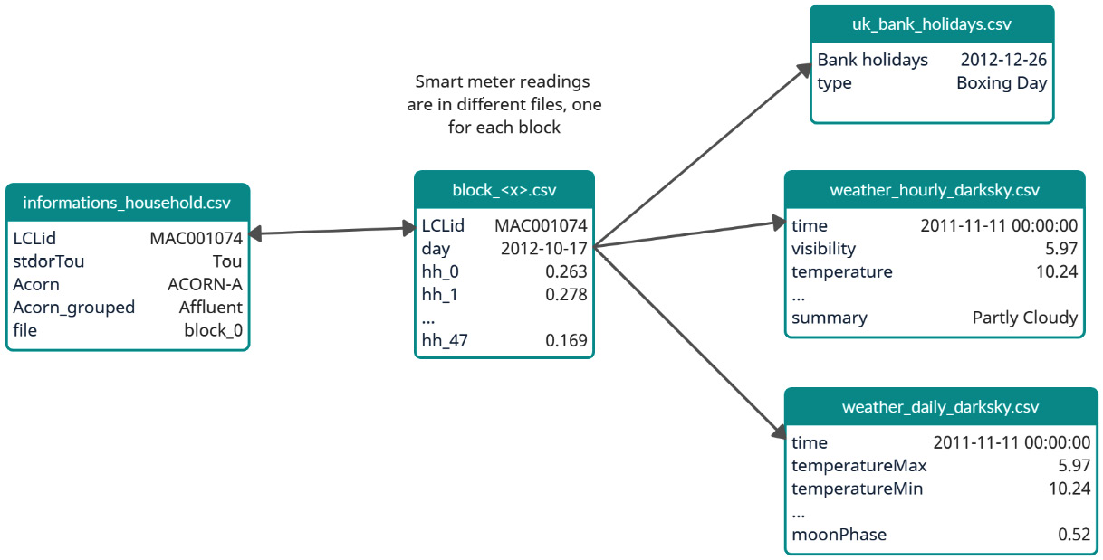
Figure 2.1 – Data model of the London Smart Meters dataset

The data model is more for us to understand the data rather than any data engineering purpose. Therefore, it only contains bare-minimum information, such as the key columns on the left and the sample data on the right. We also have arrows connecting different files, with keys used to link the files.

Let’s look at a few key column names and their meanings:

• LCLid: The unique consumer ID for a household
• stdorTou: Whether the household has dToU or standard
• Acorn: The ACORN class
• Acorn_grouped: The ACORN group
• file: The block number

Each LCLid has a unique time series attached to it. The time series file is formatted in a slightly tricky format – each day, there will be 48 observations at a half-hourly frequency in the columns of the file.

Notebook alert

To follow along with the complete code, use the 01 - Pandas Refresher & Missing Values Treatment.ipynb notebook in the chapter01 folder.

Before we start working with our dataset, there are a few concepts we need to establish. One of them is a concept in pandas DataFrames, which is of utmost importance – the pandas datetime properties and index. Let’s quickly look at a few pandas concepts that will be useful.

Important note

If you are familiar with the datetime manipulations in pandas, feel free to skip ahead to the next section.

pandas datetime operations, indexing, and slicing 
– a refresher

Instead of using our dataset, which is slightly complex, let’s pick an easy, well-formatted stock exchange price dataset from the UCI Machine Learning Repository and look at the functionality of pandas:

df = pd.read_excel("https://archive.ics.uci.edu/ml/machine-learning-databases/00247/data_akbilgic.xlsx", skiprows=1)

The DataFrame that we read looks as follows:

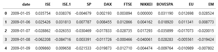
Figure 2.2 – The DataFrame with stock exchange prices

Now that we have read the DataFrame, let’s start manipulating it.

Converting the date columns into pd.Timestamp/DatetimeIndex

First, we must convert the date column (which may not always be parsed as dates automatically by pandas) into pandas datetime. For that, pandas has a handy function called pd.to_datetime. It infers the datetime format automatically and converts the input into a pd.Timestamp, if the input is a string, or into a DatetimeIndex if the input is a list of strings. So, if we pass a single date as a string, pd.to_datetime converts it into pd.Timestamp, while if we pass a list of dates, it converts it into DatetimeIndex:

>>> pd.to_datetime("13-4-1987").strftime("%d, %B %Y")
'13, April 1987'

Now, let’s look at a case where the automatic parsing fails. The date is January 4, 1987. Let’s see what happens when we pass the string to the function:

>>> pd.to_datetime("4-1-1987").strftime("%d, %B %Y")
'01, April 1987'

Well, that wasn’t expected, right? But if you think about it, anyone can make that mistake because we are not telling the computer whether the month or the day comes first, and pandas assumes the month comes first. Let’s rectify that:

>>> pd.to_datetime("4-1-1987", dayfirst=True).strftime("%d, %B %Y")
'04, January 1987'

Another case where automatic date parsing fails is when the date string is in a non-standard form. In that case, we can provide a strftime formatted string to help pandas parse the dates correctly:

>>> pd.to_datetime("4|1|1987", format="%d|%m|%Y").strftime("%d, %B %Y")
'04, January 1987'

A full list of strftime conventions can be found at https://strftime.org/.

Practitioner’s tip

Because of the wide variety of data formats, pandas may infer the time incorrectly. While reading a file, pandas will try to parse the dates automatically and create an error. There are many ways we can control this behavior: we can use the parse_dates flag to turn off date parsing, the date_parser argument to pass in a custom date parser, and year_first and day_first to easily denote two popular formats of dates.

Out of all these options, I prefer to use parse_dates=False in both pd.read_csv and pd.read_excel to make sure pandas is not parsing the data automatically. After that, you can convert the date using the format parameter, which lets you explicitly set the date format of the column using strftime conventions. There are two other parameters in pd.to_datetime that will also make inferring dates less error-prone – yearfirst and dayfirst. If you don’t provide an explicit date format, at least provide one of these.

Now, let’s convert the date column in our stock prices dataset into datetime:

df['date'] = pd.to_datetime(df['date'], yearfirst=True)

Now, the 'date' column, dtype, should be either datetime64[ns] or <M8[ns], which are both pandas/NumPy native datetime formats. But why do we need to do this?

It’s because of the wide range of additional functionalities this unlocks. The traditional min() and max() functions will start working because pandas knows it is a datetime column:

>>> df.date.min(),df.date.max()
(Timestamp('2009-01-05 00:00:00'), Timestamp('2011-02-22 00:00:00'))

Let’s look at a few cool features the datetime format gives us.

Using the .dt accessor and datetime properties

Since the column is now in date format, all the semantic information that is encoded in the date can be used through pandas datetime properties. We can access many datetime properties, such as month, day_of_week, day_of_year, and so on, using the .dt accessor:

>>> print(f"""
     Date: {df.date.iloc[0]}
     Day of year: {df.date.dt.day_of_year.iloc[0]}
     Day of week: {df.date.dt.dayofweek.iloc[0]}
     Week of Year: {df.date.dt.weekofyear.iloc[0]}
     Month: {df.date.dt.month.iloc[0]}
     Month Name: {df.date.dt.month_name().iloc[0]}
     Quarter: {df.date.dt.quarter.iloc[0]}
     Year: {df.date.dt.year.iloc[0]}
     ISO Week: {df.date.dt.isocalendar().week.iloc[0]}
     """)
Date: 2009-01-05 00:00:00
Day of year: 5
Day of week: 0
Week of Year: 2
Month: 1
Month Name: January
Quarter: 1
Year: 2009
ISO Week: 2

As of pandas 1.1.0, week_of_year has been deprecated because of the inconsistencies it produces at the end/start of the year. Instead, the ISO Calendar standards (which are commonly used in government and business) have been adopted and we can access the ISO calendar to get the ISO weeks.

Slicing and indexing

The real fun starts when we make the date column the index of the DataFrame. By doing this, you can use all the fancy slicing operations that pandas supports but on the datetime axis. Let’s take a look at few of them:

# Setting the index as the datetime column
df.set_index("date", inplace=True)
# Select all data after 2010-01-04(including)
df["2010-01-04":]
# Select all data between 2010-01-04 and 2010-02-06(not including)
df["2010-01-04": "2010-02-06"]
# Select data 2010 and before
df[: "2010"]
# Select data between 2010-01 and 2010-06(both including)
df["2010-01": "2010-06"]

In addition to the semantic information and intelligent indexing and slicing, pandas also provides tools for creating and manipulating date sequences.

Creating date sequences and managing date offsets

If you are familiar with range in Python and np.arange in NumPy, then you will know they help us create integer/float sequences by providing a start point and an end point. pandas has something similar for datetime – pd.date_range. The function accepts start and end dates, along with a frequency (daily or monthly, and so on) and creates the sequence of dates in between. Let’s look at a couple of ways of creating a sequence of dates:

# Specifying start and end dates with frequency
pd.date_range(start="2018-01-20", end="2018-01-23", freq="D").astype(str).tolist()
# Output: ['2018-01-20', '2018-01-21', '2018-01-22', '2018-01-23']
# Specifying start and number of periods to generate in the given frequency
pd.date_range(start="2018-01-20", periods=4, freq="D").astype(str).tolist()
# Output: ['2018-01-20', '2018-01-21', '2018-01-22', '2018-01-23']
# Generating a date sequence with every 2 days
pd.date_range(start="2018-01-20", periods=4, freq="2D").astype(str).tolist()
# Output: ['2018-01-20', '2018-01-22', '2018-01-24', '2018-01-26']
# Generating a date sequence every month. By default it starts with Month end
pd.date_range(start="2018-01-20", periods=4, freq="M").astype(str).tolist()
# Output: ['2018-01-31', '2018-02-28', '2018-03-31', '2018-04-30']
# Generating a date sequence every month, but month start
pd.date_range(start="2018-01-20", periods=4, freq="MS").astype(str).tolist()
# Output: ['2018-02-01', '2018-03-01', '2018-04-01', '2018-05-01']

We can also add or subtract days, months, and other values to/from dates using pd.TimeDelta:

# Add four days to the date range
(pd.date_range(start="2018-01-20", end="2018-01-23", freq="D") + pd.Timedelta(4, unit="D")).astype(str).tolist()
# Output: ['2018-01-24', '2018-01-25', '2018-01-26', '2018-01-27']
# Add four weeks to the date range
(pd.date_range(start="2018-01-20", end="2018-01-23", freq="D") + pd.Timedelta(4, unit="W")).astype(str).tolist()
# Output: ['2018-02-17', '2018-02-18', '2018-02-19', '2018-02-20']

There are a lot of these aliases in pandas, including W, W-MON, MS, and others. The full list can be found at https://pandas.pydata.org/docs/user_guide/timeseries.html#timeseries-offset-aliases.

In this section, we looked at a few useful features and operations we can perform on datetime indices and know how to manipulate DataFrames with datetime columns. Now, let’s review a few techniques we can use to deal with missing data.

Handling missing data

While dealing with large datasets in the wild, you are bound to encounter missing data. If it is not part of the time series, it may be part of the additional information you collect and map. Before we jump the gun and fill it with a mean value or drop those rows, let’s think about a few aspects:

• The first consideration should be whether the missing data we are worried about is missing or not. For that, we need to think about the Data Generating Process (DGP) (the process that is generating the time series). As an example, let’s look at sales at a local supermarket. You have been given the point-of-sale (POS) transactions for the last 2 years and you are processing the data into a time series. While analyzing the data, you found that there are a few products where there aren’t any transactions for a few days. Now, what you need to think about is whether the missing data is missing or whether there is some information that this missingness is giving you. If you don’t have any transactions for a particular product for a day, it will appear as missing data while you are processing it, even though it is not missing. What that tells us you that there were no sales for that item, and that you should fill such missing data with zeros.
• Now, what if you see that, every Sunday, the data is missing – that is, there is a pattern to the missingness. This becomes tricky because how you fill in such gaps depends on the model that you intend to use. If you fill in such gaps with zeros, a model that looks at the immediate past to predict the future will predict inaccurate results on Monday. However, if you tell the model that the previous day was Sunday, then the model still can learn to tell the difference.
• Lastly, what if you see zero sales on one of the best-selling products that always gets sold? This can happen because of something such as a POS machine malfunction, a data entry mistake, or an out-of-stock situation. These types of missing values can be imputed with a few techniques.

Let’s look at an Air Quality dataset published by the ACT Government, Canberra, Australia under the CC by Attribution 4.0 International License (https://www.data.act.gov.au/Environment/Air-Quality-Monitoring-Data/94a5-zqnn) and see how we can impute such values using pandas (there are more sophisticated techniques available, all of which will be covered later in this chapter).

Practitioner’s tip

When reading data using a method such as read_csv, pandas provides a few handy ways to handle missing values. pandas treats many values such as #N/A, null, and so on as NaN by default. We can control this list of allowable NaN values using the na_values and keep_default_na parameters.

We have chosen region Monash and PM2.5 readings and introduced some missing values, as shown in the following diagram:

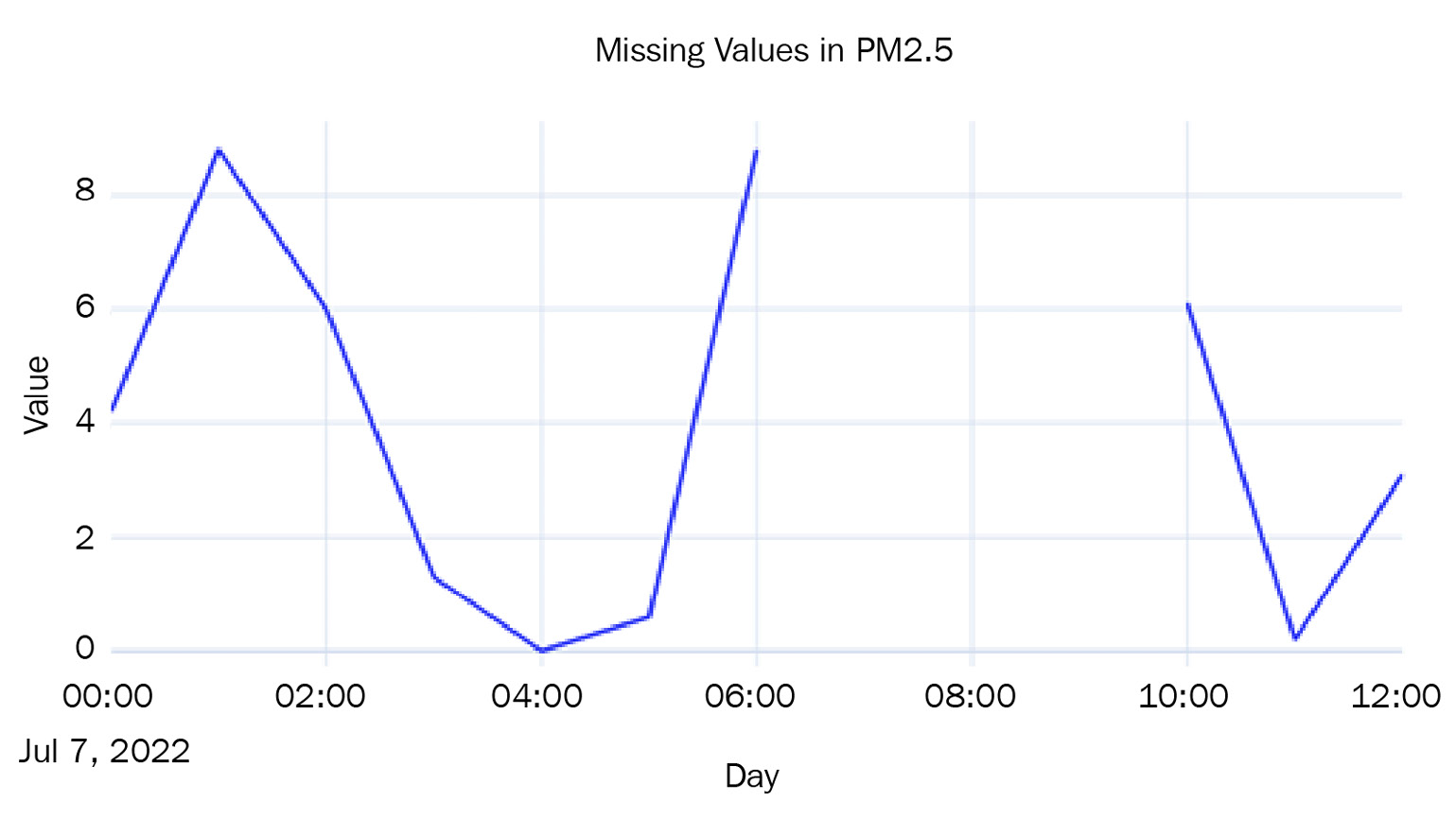
Figure 2.3 – Missing values in the Air Quality dataset

Now, let’s look at a few simple techniques we can use to fill the missing values:

• Last Observation Carried Forward or Forward Fill: This imputation technique takes the last observed value and uses that to fill all the missing values until it finds the next observation. It is also called forward fill. We can do this like so:

  df['pm2_5_1_hr'].ffill()
• Next Observation Carried Backward of Backward Fill: This imputation technique takes the next observation and backtracks to fill in all the missing values with this value. This is also called backward fill. Let’s see how we can do this in pandas:

  df['pm2_5_1_hr'].bfill()
• Mean Value Fill: This imputation technique is also pretty simple. We calculate the mean of the entire series and wherever we find missing values, we fill it with the mean value:

  df['pm2_5_1_hr'].fillna(df['pm2_5_1_hr'].mean())

Let’s plot the imputed lines we get from using these three techniques:

Figure 2.4 – Imputed missing values using forward, backward, and mean value fill

Another family of imputation techniques covers interpolation:

• Linear Interpolation: Linear interpolation is just like drawing a line between the two observed points and filling the missing values so that they lie on this line. This is how we do it:

  df['pm2_5_1_hr'].interpolate(method="linear")
• Nearest Interpolation: This is intuitively like a combination of the forward and backward fill. For each missing value, the closest observed value is found and is used to fill in the missing value:

  df['pm2_5_1_hr'].interpolate(method="nearest")

Let’s plot the two interpolated lines:

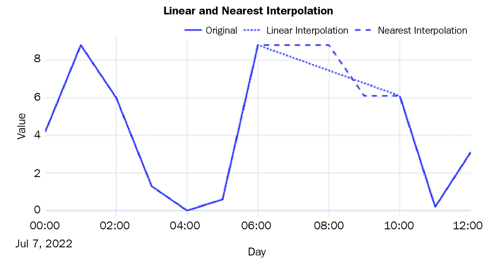
Figure 2.5 – Imputed missing values using linear and nearest interpolation

There are a few non-linear interpolation techniques as well:

• Spline, Polynomial, and Other Interpolations: In addition to linear interpolation, pandas also supports non-linear interpolation techniques that call a SciPy routine at the backend. Spline and polynomial interpolations are similar. They fit a spline/polynomial of a given order to the data and use that to fill in missing values. While using spline or polynomial as the method in interpolate, we should always provide order as well. The higher the order, the more flexible the function that is used will be to fit the observed points. Let’s see how we can use spline and polynomial interpolation:

  df['pm2_5_1_hr'].interpolate(method="spline", order=2)

  df['pm2_5_1_hr'].interpolate(method="polynomial", order=5)

Let’s plot these two non-linear interpolation techniques:

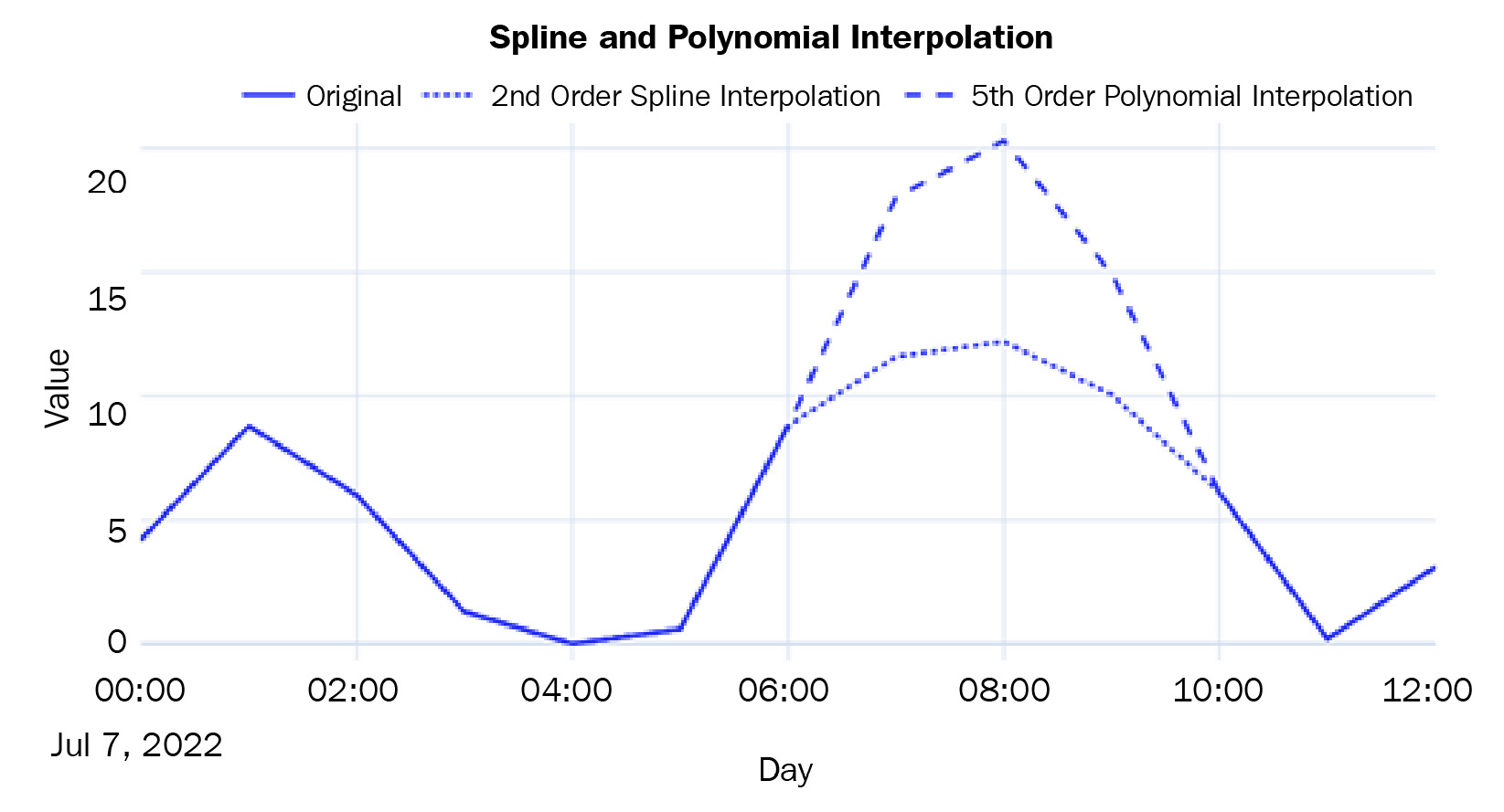
Figure 2.6 – Imputed missing values using spline and polynomial interpolation

For a complete list of interpolation techniques supported by interpolate, go to https://pandas.pydata.org/pandas-docs/stable/reference/api/pandas.Series.interpolate.html and https://docs.scipy.org/doc/scipy/reference/generated/scipy.interpolate.interp1d.html#scipy.interpolate.interp1d.

Now that we are more comfortable with the way pandas manages datetime, let’s go back to our dataset and convert the data into a more manageable form.

Notebook alert

To follow along with the complete code for pre-processing, use the 02 - Preprocessing London Smart Meter Dataset.ipynb notebook in the chapter01 folder.

Converting the half-hourly block-level data (hhblock) into time series data

Before we start processing, let’s understand a few general categories of information we will find in a time series dataset:

• Time Series Identifiers: These are identifiers for a particular time series. It can be a name, an ID, or any other unique feature – for example, the SKU name or the ID of a retail sales dataset or the consumer ID in the energy dataset that we are working with are all time series identifiers.
• Metadata or Static Features: This information does not vary with time. An example of this is the ACORN classification of the household in our dataset.
• Time-Varying Features: This information varies with time – for example, the weather information. For each point in time, we have a different value for weather, unlike the Acorn classification.

Next. Let’s discuss formatting of a dataset.

Compact, expanded, and wide forms of data

There are many ways to format a time series dataset, especially a dataset with many related time series, like the one we have now. Apart from the standard terminology of wide data, we can also look at two non-standard ways of formatting time series data. Although there is no standard nomenclature for those, we will refer to them as compact and expanded in this book.

Compact form data is when any particular time series occupies only a single row in the pandas DataFrame – that is, the time dimension is managed as an array within a DataFrame row. The time series identifiers and the metadata occupy the columns with scalar values and then the time series values; other time-varying features occupy the columns with an array. Two additional columns are included to extrapolate time – start_datetime and frequency. If we know the start datetime and the frequency of the time series, we can easily construct the time and recover the time series from the DataFrame. This only works for regularly sampled time series. The advantage is that the DataFrames take up much less memory and are easy and faster to work with:

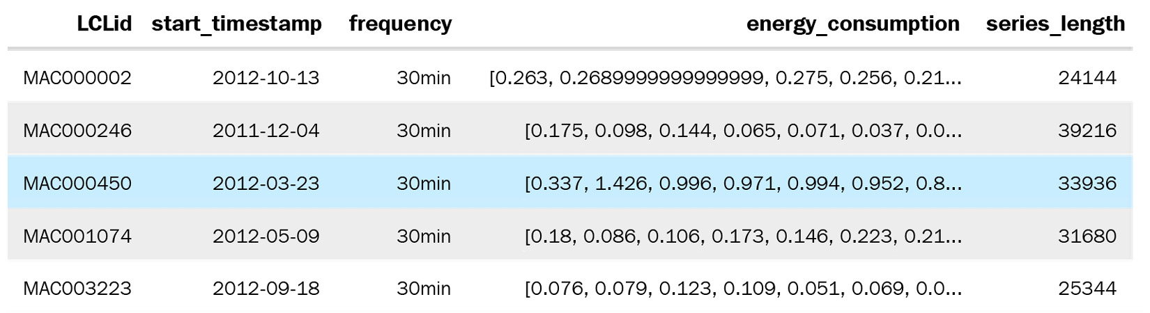
Figure 2.7 – Compact form data

The expanded form is when the time series is expanded along the rows of a DataFrame. If there are n steps in the time series, it occupies n rows in the DataFrame. The time series identifiers and the metadata get repeated along all the rows. The time-varying features also get expanded along the rows. And instead of the start date and frequency, we have the datetime as a column:

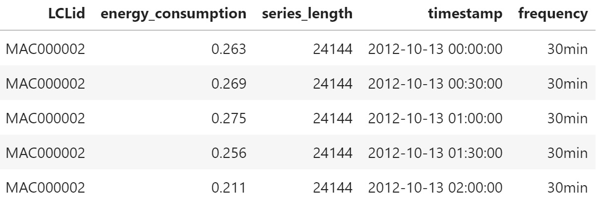
Figure 2.8 – Expanded form data

If the compact form had a time series identifier as the key, the time series identifier and the datetime column would be combined and become the key.

Wide-format data is more common in traditional time series literature. It can be considered a legacy format, which is limiting in many ways. Do you remember the stock data we saw earlier (Figure 2.2)? We have the date as an index or as one of the columns and the different time series as different columns of the DataFrame. As the number of time series increases, they become wider and wider, hence the name. This data format does not allow us to include any metadata about the time series. For instance, in our data, we have information about whether a particular household is under standard or dynamic pricing. There is no way for us to include such metadata in the wide format. From an operational perspective, the wide format also does not play well with relational databases because we have to keep adding columns to the table when we get new time series. We won’t be using this format in this book.

Enforcing regular intervals in time series

One of the first things you should check and correct is whether the regularly sampled time series data that you have has equal intervals of time. In practice, even regularly sampled time series have some samples missing in between because of some data collection error or some other peculiar way data is collected. So, while working with the data, we will make sure we enforce regular intervals in the time series.

Best practice

While working with datasets with multiple time series, it is best practice to check the end dates of all the time series. If they are not uniform, we can align them with the latest date across all the time series in the dataset.

In our smart meters dataset, some LCLid columns end much earlier than the rest. Maybe the household opted out of the program, or they moved out and left the house empty; the reason could be anything. However, we need to handle that while we enforce regular intervals.

We will learn how to convert the dataset into a time series format in the next section. The code for this process can be found in the 02 - Preprocessing London Smart Meter Dataset.ipynb notebook.

Converting the London Smart Meters dataset into a time series format

For each dataset that you come across, the steps you would have to take to convert it into either a compact or expanded form would be different. It depends on how the original data is structured. Here, we will look at how the London Smart Meters dataset can be transformed so that we can transfer those learnings to other datasets.

There are two steps we need to do before we can start processing the data into either compact or expanded form:

1. Find the Global End Date: We must find the maximum date across all the block files so that we know the global end date of the time series.
2. Basic Preprocessing: If you remember how hhblock_dataset is structured, you will remember that each row had a date and that along the columns, we have half-hourly blocks. We need to reshape that into a long form, where each row has a date and a single half-hourly block. It’s easier to handle that way.

Now, let’s define separate functions for converting the data into compact and expanded forms and apply that function to each of the LCLid columns. We will do this for each LCLid separately since the start date for each LCLid is different.

Expanded form

The function for converting into expanded form does the following:

1. Finds the start date.
2. Create a standard DataFrame using the start date and the global end date.
3. Left merges the DataFrame for LCLid to the standard DataFrame, leaving the missing data as np.nan.
4. Returns the merged DataFrame.

Once we have all the LCLid DataFrames, we must perform a couple of additional steps to complete the expanded form processing:

1. Concatenate all the DataFrames into a single DataFrame.
2. Create a column called offset, which is the numerical representation of the half-hour blocks; for example, hh_3 → 3.
3. Create a timestamp by adding a 30-minute offset to the day and dropping the unnecessary columns.

For one block, this representation takes up ~47 MB of memory.

Compact form

The function for converting into compact form does the following:

1. Finds the start date and time series identifiers.
2. Creates a standard DataFrame using the start date and the global end date.
3. Left merges the DataFrame for LCLid to the standard DataFrame, leaving the missing data as np.nan.
4. Sorts the values on the date.
5. Returns the time series array, along with the time series identifier, start date, and the length of the time series.

Once we have this information for each LCLid, we can compile it into a DataFrame and add 30min as the frequency.

For one block, this representation takes up only ~0.002 MB of memory.

We are going to use the compact form because it is easy to work with and much less resource hungry.

Mapping additional information

From the data model that we prepared earlier, we know that there are three key files that we have to map: Household Information, Weather, and Bank Holidays.

The informations_households.csv file contains metadata about the household. There are static features that are not dependent on time. For this, we just need to left merge informations_households.csv to the compact form based on LCLid, which is the time series identifier.

Best practice

While doing a pandas merge, one of the most common and unexpected outcomes is that the number of rows before and after the operation is not the same (even if you are doing a left merge). This typically happens because there are duplicates in the keys on which you are merging. As a best practice, you can use the validate parameter in the pandas merge, which takes in inputs such as one_to_one and many_to_one so that this check is done while merging and will throw an error if the assumption is not met. For more information, go to https://pandas.pydata.org/docs/reference/api/pandas.merge.html.

Bank Holidays and Weather, on the other hand, are time-varying features and should be dealt with accordingly. The most important aspect to keep in mind is that while we map this information, it should perfectly align with the time series that we have already stored as an array.

uk_bank_holidays.csv is a file that contains the dates of the holidays and the kind of holiday. The holiday information is quite important here because the energy consumption patterns would be different on a holiday when the family members are at home spending time with each other or watching television, and so on. Follow these steps to process this file:

1. Convert the date column into the datetime format and set it as the index of the DataFrame.
2. Using the resample function we saw earlier, we must ensure that the index is resampled every 30 minutes, which is the frequency of the times series.
3. Forward fill the holidays within a day and fill in the rest of the NaN values with NO_HOLIDAY.

Now, we have converted the holiday file into a DataFrame that has a row for each 30-minute interval. On each row, we have a column that specifies whether that day was a holiday or not.

weather_hourly_darksky.csv is a file that is, once again, at the daily frequency. We need to downsample it to a 30-minute frequency because the data that we need to map to this is at a half-hourly frequency. If we don’t do this, the weather will only be mapped to the hourly timestamps, leaving the half-hourly timestamps empty.

The steps we must follow to process this file are also similar to the way we processed holidays:

1. Convert the date column into the datetime format and set it as the index of the DataFrame.
2. Using the resample function, we must ensure that the index is resampled every 30 minutes, which is the frequency of the times series.
3. Forward fill the weather features to fill the missing values that were created while resampling.

Now that you have made sure the alignment between the time series and the time-varying features is ensured, you can loop over each of the time series and extract the weather and bank holiday array before storing it in the corresponding row of the DataFrame.

Saving and loading files to disk

The fully merged DataFrame in its compact form takes up only ~10 MB. But saving this file requires a little bit of engineering. If we try to save the file in CSV format, it will not work because of the way we have stored arrays in pandas columns (since the data is in its compact form). We can save it in pickle or parquet format, or any of the binary forms of file storage. This can work, depending on the size of the RAM available in our machines. Although the fully merged DataFrame is just ~10 MB, saving it in pickle format will make the size explode to ~15 GB.

What we can do is save this as a text file while making a few tweaks to accommodate the column names, column types, and other metadata that is required to read the file back into memory. The resulting file size on disk still comes out to ~15 GB but since we are doing it as an I/O operation, we are not keeping all that data in our memory. We call this the time series (.ts) format. The functions for saving a compact form in .ts format, reading the .ts format, and converting the compact form into expanded form are available in this book’s GitHub repository under src/data_utils.py.

If you don’t need to store all of the DataFrame in a single file, you can split it into multiple chunks and save them individually in a binary format, such as parquet. For our datasets, let’s follow this route and split the whole DataFrame into chunks of blocks and save them as parquet files. This is the best route for us because of a few reasons:

• It leverages the compression that comes with the format
• It reads in parts of the whole data for quick iteration and experimentation
• The data types are retained between the read and write operations, leading to less ambiguity

Now that we have processed the dataset and stored it on disk, let’s read it back into memory and look at a few more techniques to handle missing data.

Handling longer periods of missing data

We saw some techniques for handling missing data earlier – forward and backward filling, interpolation, and so on. Those techniques usually work if there are one or two missing data points. But if a large section of data is missing, then these simple techniques fall short.

Notebook alert

To follow along with the complete code for missing data imputation, use the 03 - Handling Missing Data (Long Gaps).ipynb notebook in the chapter02 folder.

Let’s read blocks 0-7 parquet from memory:

block_df = pd.read_parquet("data/london_smart_meters/preprocessed/london_smart_meters_merged_block_0-7.parquet")

The data that we have saved is in compact form. We need to convert it into expanded form because it is easier to work with time series data in that form. Since we only need a subset of the time series (for faster demonstration purposes), we are just extracting one block from these seven blocks. To convert compact form into expanded form, we can use a helpful function in src/utils/data_utils.py called compact_to_expanded:

#Converting to expanded form
exp_block_df = compact_to_expanded(block_df[block_df.file=="block_7"], timeseries_col = 'energy_consumption',
static_cols = ["frequency", "series_length", "stdorToU", "Acorn", "Acorn_grouped", "file"],
time_varying_cols = ['holidays', 'visibility', 'windBearing', 'temperature', 'dewPoint',
       'pressure', 'apparentTemperature', 'windSpeed', 'precipType', 'icon',
       'humidity', 'summary'],
ts_identifier = "LCLid")

One of the best ways to visualize the missing data in a group of related time series is by using a very helpful package called missingno:

# Pivot the data to set the index as the datetime and the different time series along the columns
plot_df = pd.pivot_table(exp_block_df, index="timestamp", columns="LCLid", values="energy_consumption")
# Generate Plot. Since we have a datetime index, we can mention the frequency to decide what do we want on the X axis
msno.matrix(plot_df, freq="M")

The preceding code produces the following output:

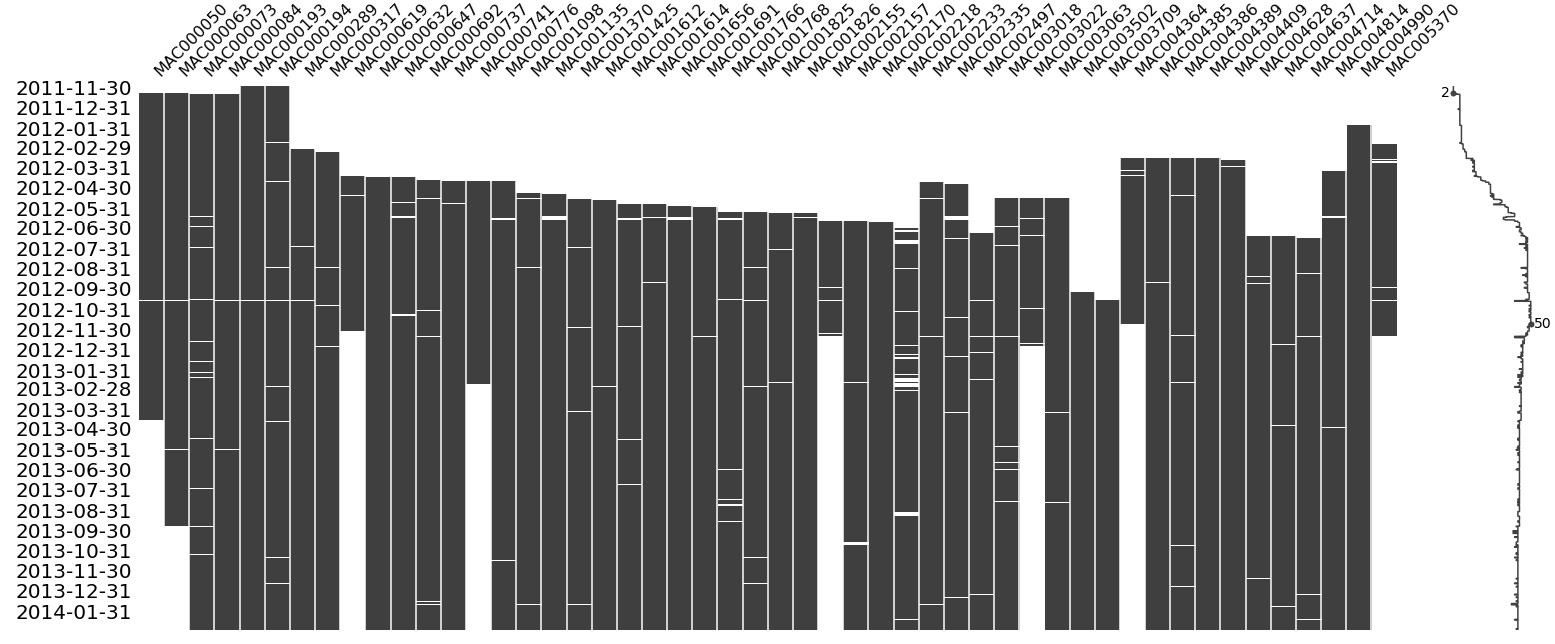
Figure 2.9 – Visualization of the missing data in block 7

Important note

Only attempt the missingno visualization on related time series where there are less than 25 time series. If you have a dataset that contains thousands of time series (such as in our full dataset), applying this visualization will give us an illegible plot and a frozen computer.

This visualization tells us a lot of things at a single glance. The Y-axis contains the dates that we are plotting the visualization for, while the X-axis contains the columns, which in this case are the different households. We know that all the time series are not perfectly aligned – that is, not all of them start at the same time and end at the same time. The big white gaps we can see at the beginning of many of the time series show that data collection for those consumers started later than the others. We can also see that a few time series finish earlier than the rest, which means either they stopped being consumers or the measurement phase stopped. There are also a few smaller white lines in many time series, which are real missing values. We can also notice a sparkline to the right, which is a compact representation of the number of missing columns for each row. If there are no missing values (all time series have some value), then the sparkline would be at the far right. Finally, if there are a lot of missing values, the line will be to the left.

Just because there are missing values, we are not going to fill/impute them because the decision of whether to impute missing data or not comes later in the workflow. For some models, we do not need to do the imputation, while for others, we do. There are multiple ways of imputing missing data and which one to choose is another decision we cannot make beforehand.

So, for now, let’s pick one LCLid and dig deeper. We already know that there are some missing values between 2012-09-30 and 2012-10-31. Let’s visualize that period:

# Taking a single time series from the block
ts_df = exp_block_df[exp_block_df.LCLid=="MAC000193"].set_index("timestamp")
msno.matrix(ts_df["2012-09-30": "2012-10-31"], freq="D")

The preceding code produces the following output:

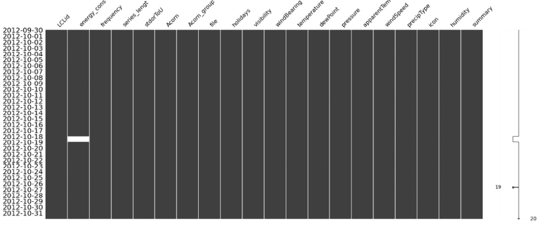
Figure 2.10 – Visualization of missing data of MAC000193 between 2012-09-30 and 2012-10-31

Here, we can see that the missing data is really between 2012-10-18 and 2012-10-19. Normally, we would go ahead and impute the missing data in this period, but since we are looking at this with an academic lens, we will take a slightly different route. Let’s introduce an artificial missing data section and see how the different techniques we are going to look at impute the missing data:

# The dates between which we are nulling out the time series
window = slice("2012-10-07", "2012-10-08")
# Creating a new column and artificially creating missing values
ts_df['energy_consumption_missing'] = ts_df.energy_consumption
ts_df.loc[window, "energy_consumption_missing"] = np.nan

Now, let’s plot the missing area in the time series:

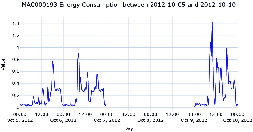
Figure 2.11 – The energy consumption of MAC000193 between 2012-10-05 and 2012-10-10

We are missing 2 whole days of energy consumption readings, which means there are 96 missing data points (half-hourly). If we use one of the techniques we saw earlier, such as interpolation, we will see that it will mostly be a straight line because none of the methods are complex enough to capture the pattern over a long time.

There are a few techniques that we can use to fill in such large missing gaps in data. We will cover these now.

Imputing with the previous day

Since this is a half-hourly time series of energy consumption, it stands to reason that there might be a pattern that is repeating day after day. The energy consumption between 9:00 A.M. and 10:00 A.M. might be higher as everybody gets ready to go to the office and a slump during the day when most houses may be empty. So, the simplest way to fill in the missing data would be to use the last day energy readings so that the energy reading at 10:00 A.M. 2012-10-18 can be filled with the energy reading at 10:00 A.M. 2012-10-17:

#Shifting 48 steps to get previous day
ts_df["prev_day"] = ts_df['energy_consumption'].shift(48)
#Using the shifted column to fill missing
ts_df['prev_day_imputed'] =  ts_df['energy_consumption_missing']
ts_df.loc[null_mask,"prev_day_imputed"] = ts_df.loc[null_mask,"prev_day"]
mae = mean_absolute_error(ts_df.loc[window, "prev_day_imputed"], ts_df.loc[window, "energy_consumption"])

Let’s see what the imputation looks like:

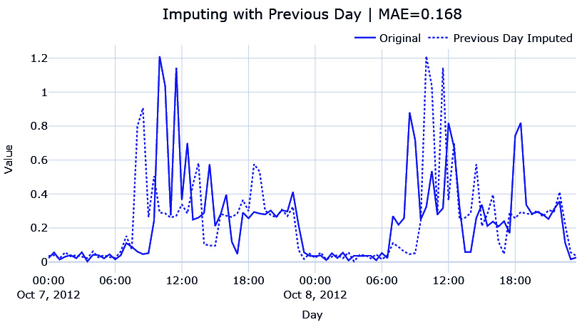
Figure 2.12 – Imputing with the previous day

While this looks better, this is also very brittle. When we are copying the previous day, we are also assuming that any kind of variation or anomalous behavior is also repeated. We can already see that the patterns for the day before and the day after are not the same.

Hourly average profile

A better approach would be to calculate an hourly profile from the data – the mean consumption for every hour – and use the average to fill the missing data:

#Create a column with the Hour from timestamp
ts_df["hour"] = ts_df.index.hour
#Calculate hourly average consumption
hourly_profile = ts_df.groupby(['hour'])['energy_consumption'].mean().reset_index()
hourly_profile.rename(columns={"energy_consumption": "hourly_profile"}, inplace=True)
#Saving the index because it gets lost in merge
idx = ts_df.index
#Merge the hourly profile dataframe to ts dataframe
ts_df = ts_df.merge(hourly_profile, on=['hour'], how='left', validate="many_to_one")
ts_df.index = idx
#Using the hourly profile to fill missing
ts_df['hourly_profile_imputed'] = ts_df['energy_consumption_missing']
ts_df.loc[null_mask,"hourly_profile_imputed"] = ts_df.loc[null_mask,"hourly_profile"]
mae = mean_absolute_error(ts_df.loc[window, "hourly_profile_imputed"], ts_df.loc[window, "energy_consumption"])

Let’s see if this is better:

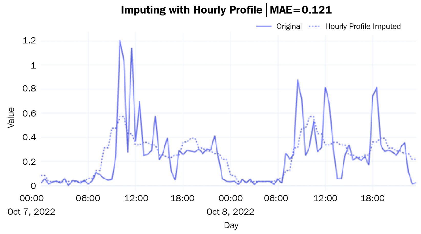
Figure 2.13 – Imputing with an hourly profile

This is giving us a much more generalized curve that does not have the spikes that we saw for the individual days. The hourly ups and downs have also been captured as per our expectations. The mean absolute error (MAE) is also lower than before.

The hourly average for each weekday

We can further refine this rule by introducing a specific profile for each weekday. It stands to reason that the usage pattern on a weekday is not going to be the same on a weekend. Hence, we can calculate the average hourly consumption for each weekday separately so that we have one profile for Monday, another for Tuesday, and so on:

#Create a column with the weekday from timestamp
ts_df["weekday"] = ts_df.index.weekday
#Calculate weekday-hourly average consumption
day_hourly_profile = ts_df.groupby(['weekday','hour'])['energy_consumption'].mean().reset_index()
day_hourly_profile.rename(columns={"energy_consumption": "day_hourly_profile"}, inplace=True)
#Saving the index because it gets lost in merge
idx = ts_df.index
#Merge the day-hourly profile dataframe to ts dataframe
ts_df = ts_df.merge(day_hourly_profile, on=['weekday', 'hour'], how='left', validate="many_to_one")
ts_df.index = idx
#Using the day-hourly profile to fill missing
ts_df['day_hourly_profile_imputed'] = ts_df['energy_consumption_missing']
ts_df.loc[null_mask,"day_hourly_profile_imputed"] = ts_df.loc[null_mask,"day_hourly_profile"]
mae = mean_absolute_error(ts_df.loc[window, "day_hourly_profile_imputed"], ts_df.loc[window, "energy_consumption"])

Let’s see what this looks like:

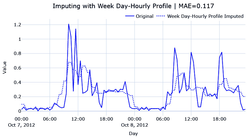
Figure 2.14 – Imputing the hourly average for each weekday

This looks very similar to the other one, but this is because the day we are imputing is a weekday and the weekday profiles are similar. The MAE is also lower than the day profile. The weekend profile is slightly different, which you can see in the associated Jupyter Notebook.

Seasonal interpolation

Although calculating seasonal profiles and using them to impute works well, there are instances, especially when there is a trend in the time series, where such a simple technique falls short. The simple seasonal profile doesn’t capture the trend at all and ignores it completely. For such cases, we can do the following:

1. Calculate the seasonal profile, similar to how we calculated the averages earlier.
2. Subtract the seasonal profile and apply any of the interpolation techniques we saw earlier.
3. Add the seasonal profile back to the interpolated series.

This process has been implemented in this book’s GitHub repository in the src/imputation/interpolation.py file. We can use it as follows:

from src.imputation.interpolation import SeasonalInterpolation
# Seasonal interpolation using 48*7 as the seasonal period.
recovered_matrix_seas_interp_weekday_half_hour = SeasonalInterpolation(seasonal_period=48*7,decomposition_strategy="additive", interpolation_strategy="spline", interpolation_args={"order":3}, min_value=0).fit_transform(ts_df.energy_consumption_missing.values.reshape(-1,1))
ts_df['seas_interp_weekday_half_hour_imputed'] = recovered_matrix_seas_interp_weekday_half_hour

The key parameter here is seasonal_period, which tells the algorithm to look for patterns that repeat every seasonal_period. If we mention seasonal_period=48, it will look for patterns that repeat every 48 data points. In our case, they are after each day (because we have 48 half-hour timesteps in a day). In addition to this, we need to specify what kind of interpolation we need to perform.

Additional information

Internally, we use something called seasonal decomposition (statsmodels.tsa.seasonal.seasonal_decompose), which will be covered in Chapter 3, Analyzing and Visualizing Time Series Data, to isolate the seasonality component.

Here, we have done seasonal interpolation using 48 (half-hourly) and 48*7 (weekday to half-hourly) and plotted the resulting imputation:

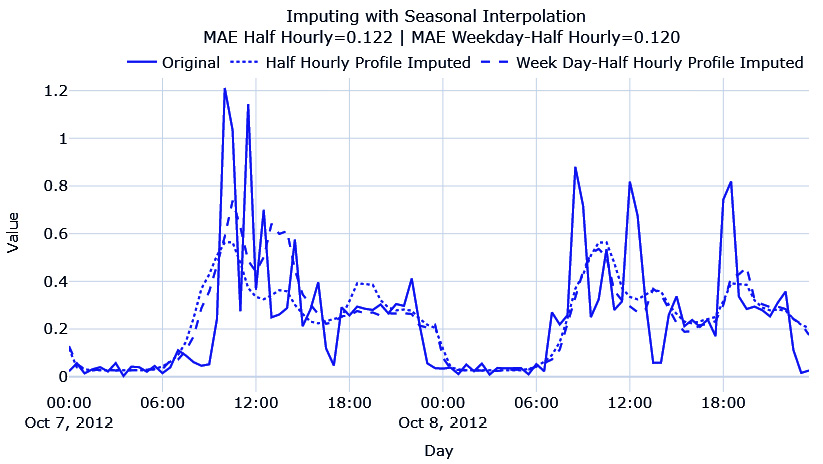
Figure 2.15 – Imputing with seasonal interpolation

Here, we can see that both have captured the seasonality patterns, but the half-hourly profile every weekday has captured the peaks in the first day better, so they have a lower MAE. There is no improvement in terms of hourly averages, mostly because there is no strong increasing or decreasing patterns in the time series.

With this, we have come to the end of this chapter. We are now officially into the nitty-gritty of juggling time series data, cleaning it, and processing it. Congratulations on finishing this chapter!

Summary

After a short refresher on pandas DataFrames, especially on the datetime manipulations and simple techniques for handling missing data, we learned about the two forms of storing and working with time series data – compact and expanded. With all this knowledge, we took our raw dataset and built a pipeline to convert it into compact form. If you have run the accompanying notebook, you should have the preprocessed dataset saved on disk. We also had an in-depth look at some techniques for handling long gaps of missing data.

Now that we have the processed datasets, in the next chapter, we will learn how to visualize and analyze a time series dataset.