14

Attention and Transformers for Time Series

In the previous chapter, we rolled up our sleeves and implemented a few deep learning (DL) systems for time series forecasting. We used the common building blocks we discussed in Chapter 12, Building Blocks of Deep Learning for Time Series, put them together in an encoder-decoder architecture, and trained them to produce the forecast we desired.

Now, let’s talk about another key concept in DL that has taken the field by storm over the past few years—attention. Attention has a long-standing history, which has culminated in it being one of the most sought-after tools in the DL toolkit. This chapter takes you on a journey to understand attention and transformer models from the ground up from a theoretical perspective and solidify that understanding with practical examples.

In this chapter, we will be covering these main topics:

• What is attention?
• Generalized attention model
• Forecasting with sequence-to-sequence models and attention
• Transformers – Attention is all you need
• Forecasting with Transformers

Technical requirements

If you have not set up the Anaconda environment following the instructions in the Preface, please do that in order to get a working environment with all the packages and datasets required for the code in this book.

You need to run the following notebooks for this chapter:

• 02 - Preprocessing London Smart Meter Dataset.ipynb in Chapter02
• 01-Setting up Experiment Harness.ipynb in Chapter04
• 01-Feature Engineering.ipynb in Chapter06
• 02-One-Step RNN.ipynb and 03-Seq2Seq RNN.ipynb in Chapter13 (for benchmarking)
• 00-Single Step Backtesting Baselines.ipynb and 01-Forecasting with ML.ipynb in Chapter08

The associated code for the chapter can be found at https://github.com/PacktPublishing/Modern-Time-Series-Forecasting-with-Python-/tree/main/notebooks/Chapter14.

What is attention?

The idea of attention was inspired by human cognitive function. At any moment, the optic nerves in our eyes, the olfactory nerves in our noses, and the auditory nerves in our ears send a massive amount of sensory input to the brain. This is way too much information, definitely more than the brain can handle. But our brains have developed a mechanism that helps us to pay attention to only the stimuli that matter—such as a sound or a smell that doesn’t belong. Years of evolution have trained our brains to pick out anomalous sounds or smells because that was key for us surviving in the wild where predators roamed free.

Apart from this kind of instinctive attention, we are also able to control our attention by what we call focusing on something. You are doing it right now by choosing to ignore all the other stimuli that you are getting and focusing your attention on the contents of this book. While you are reading, your mobile phone pings you, and the screen lights up. And your brain decides to focus its attention on the mobile screen, even though the book is still open in front of you. This feature of the human cognitive function has been the inspiration behind the attention mechanism in DL. Giving learning machines the ability to acquire this kind of attention has led to big breakthroughs in all fields of AI today.

The idea was first applied to DL in Seq2Seq models, which we learned about in Chapter 13, Common Modeling Patterns for Time Series. In the chapter, we saw how the handshake between the encoder and decoder was done. For the recurrent neural network (RNN) family of models, we use the hidden states from the encoder at the end of the sequence as the initial hidden states in the decoder. Let’s call this handshake—the context. The assumption here is that all the information required for the decoding task is encoded in the context. This creates a kind of information bottleneck (Figure 14.1). There may be information in previous hidden states that can be useful for the decoding task. In 2015, Bahdanau et al. proposed the first known attention model in the context of DL. They proposed to learn attention weights, , for each hidden state corresponding to the input sequence and combine them into a single context vector while decoding. And these attention weights are re-calculated for each decoding step using the similarity between the hidden states during decoding and all the hidden states in the input sequence (Figure 14.2):

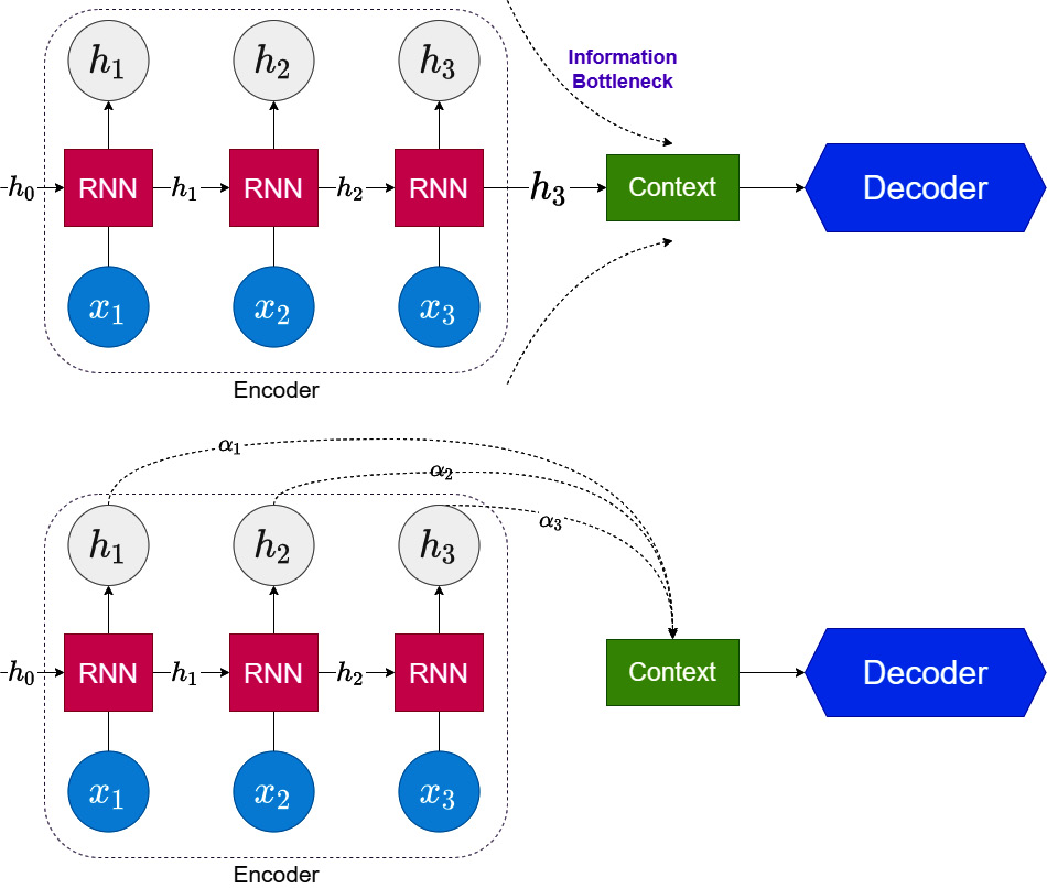
Figure 14.1 – Traditional (top) versus attention model (bottom) in Seq2Seq models

To make things clearer, let’s adopt a formal way of describing the mechanism. Let be the hidden states generated during the encoding process and be the hidden states generated during decoding. The context vector will be :

Figure 14.2 – Decoding using attention

So, now we have the hidden states from the encoding stage (), and we need to have a way to use this information at each step of decoding. The key here is that at each step of the decoding process, information from different hidden states might be relevant. And this is exactly what attention weights do. So, for decoding step , we use and calculate attention weights (we’ll look at how attention weights are learned in detail soon) , using the similarity between and each hidden state in . Now, we calculate the context vector, which combines the information in in the right way:

There are two main ways we can use this context vector, which we will go into in detail later in the chapter. This breaks the information bottleneck that was present in the traditional Seq2Seq model and allows the models to access a larger pool of information and decide which information is relevant at each step of the decoding process.

Now, let’s see how these attention weights, , are calculated.

The generalized attention model

Over the course of years, researchers have come up with different ways of calculating attention weights and using attention in DL models. Sneha Choudhari et al. published a survey paper on attention models that proposes a generalized attention model that tries to incorporate all the variations in a single framework. Let’s structure our discussion around this generalized framework.

We can think of an attention model as learning an attention distribution () for a set of keys, K, using a set of queries, q. In the example we discussed in the last section, the query would be —the hidden state from the last timestep during decoding—and the keys would be —all the hidden states generated using the input sequence. In some cases, the generated attention distribution is applied to another set of inputs called values, V. In many cases, K and V are the same, but to maintain the general form of the framework, we consider these separately. Using these terminologies, we can define an attention model as a function of q, K, and V:

Here, is an alignment function that calculates a similarity or a notion of similarity between the queries and keys. In the example we discussed in the previous section, this alignment function calculates how relevant an encoder hidden state is to a decoder hidden state, and is a distribution function that converts this score into attention weights that sum up to 1.

Reference check

The research papers by Sneha Choudhari et al. are cited in the References section under 8.

Since we have the generalized attention model now, let’s also see how we can implement this in PyTorch. The full implementation can be found in the Attention class in src/dl/attention.py, but we will cover the key parts of it here.

The only information we require beforehand to initialize such a module is the hidden dimension of the queries and keys (encoder and decoder). So, the class definition and the __init__ function of the class look like this:

class Attention(nn.Module, metaclass=ABCMeta):
    def __init__(self, encoder_dim: int, decoder_dim: int):
        super().__init__()
        self.encoder_dim = encoder_dim
        self.decoder_dim = decoder_dim

Now, we need to define a forward function, which takes in two inputs:

• query: The query vector of size (batch size, decoder dimension), which we are going to use to find the attention weights with which to combine the keys. This is the in .
• key: The key vector of size (batch size, sequence length, encoder dimension), which is the sequence of hidden states across which we will be calculating the attention weights. This is the in .

We are assuming keys and values are the same because in most cases, they are. So, from the generalized attention model, we know that there are a few steps we need to perform:

1. Calculate an alignment score——for each query and key combination.
2. Convert the scores to weights by applying a function—.
3. Use the learned weights to combine the values—.

So, let’s see those steps in code in the forward method:

def forward(
        self,
        query: torch.Tensor,  # [batch_size, decoder_dim]
        values: torch.Tensor,  # [batch_size, seq_length, encoder_dim]
    ):
        scores = self._get_scores(query, values)  # [batch_size, seq_length]
        weights = torch.nn.functional.softmax(scores, dim=-1)
        return (values*weights.unsqueeze(-1)).sum(dim=1)  # [batch_size, encoder_dim]

The three lines of code in the forward method correspond to the three steps we discussed earlier. The first step, which is calculating the scores, is the key step that has led to many different types of attention, and therefore we have generalized that into a _get_scores abstract method that must be implemented by any class inheriting the Attention class. For the second line, we have used the softmax function for converting the scores to weights, and in the last line, we are doing an element-wise multiplication (*) between weights and values and summing across the sequence length to get the weighted value.

Now let’s turn our attention toward alignment functions.

Alignment functions

There are many variations of the alignment function that have come up over the years. Let’s review a few popular ones that are used today.

Dot product

This is probably the simplest alignment function of all. Luong et al. proposed this form of attention in 2015. From linear algebra intuition, we know that a dot product between two vectors tells us what amount of one vector goes in the direction of another. It measures some kind of similarity between the two vectors, and this similarity considers both the magnitude of the vectors and the angle between them in the vector space. Therefore, when we take a dot product between our query and key vectors, we get a notion of similarity between them. One thing to note here is that the hidden dimensions of the query and key should be the same for dot product attention to be applied. Formally, the similarity function can be defined as follows:

We need to calculate this score for each of the elements in the key, , and instead of running a loop over each element in K, we can use a clever matrix multiplication trick to calculate the scores for all the keys in K in one shot. Let’s see how we can define the _get_scores function for dot product attention.

We know from the previous section that the query and values (which are the same as keys in our case) are of (batch size, decoder dimension) and (batch size, sequence length, encoder dimension) dimensions respectively, and will be called q and v in the _get_scores function. And in this particular case, the decoder dimension and the encoder dimension are the same, so the scores can be calculated as follows:

scores = (q @ v.transpose(1,2))

Here, @ is shorthand for torch.matmul, which does matrix multiplication. The entire implementation is named DotProductAttention and can be found in src/dl/attention.py.

Scaled dot product attention

In 2017, Vaswani et al. proposed this type of attention in the seminal paper, Attention is All you Need. We will delve into that paper later in this chapter, but now, let’s understand one key modification they suggested to the dot product attention. The modification is motivated by the concern that when the input is large, the softmax function we use to convert scores to weights may have very small gradients and hence makes efficient learning difficult.

This is because the softmax function is not scale-invariant. The exponential function in the softmax function is the reason for this behavior. So, the higher we scale the inputs to the function, the more the largest input dominates the output, and this throttles the gradient flow in the network. If we assume and are dimensional vectors with 0 mean and a variance of 1, then their dot product would have a mean of zero and a variance of . Therefore, if we scale the output of the dot product by , then we bring the variance of the dot product back to 1. So, by controlling for the scale of the inputs to the softmax function, we manage a healthy gradient flow through the network. The Further reading section has a link to a blog post that goes into this in more depth. Therefore, the scaled dot product alignment function can be defined as follows:

And consequently, the only change we will have to make in the PyTorch implementation is one additional line:

scores = scores/math.sqrt(encoder_dim)

This has been implemented as a parameter in DotProductAttention in src/dl/attention.py. If you pass scaled=True while initializing the class, it will perform scaled dot product attention. We need to keep in mind that similar to dot product attention, the scaled variant also requires the query and values to have the same dimensions.

General attention

In 2015, Luong et al. also proposed a slight variation of dot product attention by introducing a learnable matrix into the calculation. They called it general attention. We can think of it as an attention mechanism that allows for the query to be projected into a learned plane of the same dimension as the values/keys using the matrix before computing the similarity score using a dot product. The alignment function can be written as follows:

The corresponding PyTorch implementation can be found under the name GeneralAttention in src/dl/attention.py. The key line calculating the attention scores can be written as follows:

scores = (q @ self.W) @ v.transpose(1,2)

Here, self.W is a tensor of size (encoder hidden dimension x decoder hidden dimension). General attention can be used in cases where the query and key/value dimensions are different.

Additive/concat attention

In 2015, Bahdanau et al. proposed additive attention, which was one of the first attempts at introducing attention to DL systems. Instead of using a defined similarity function such as the dot product, Bahdanau et al. proposed that the similarity function can be learned, giving the network more flexibility in deciding what it deems to be similar. They suggested that we can concatenate the query and the key into a single tensor and use a learnable matrix, , to calculate the attention scores. This alignment function can be written as follows:

Here, , and are learnable matrices. In cases where the query and key have different hidden dimensions, we can use and to project them into a single dimension and then perform a similarity calculation on them. In the case that the query and key have the same hidden dimension, this is also equivalent to the variant of attention used in Luong et al., which they call concat attention, represented as follows:

It is simple linear algebra to see that both are the same and for engineering simplicity. The Further reading section has a link to a Stack Overflow answer that explains the equivalence.

We have included both implementations in src/dl/attention.py under ConcatAttention and AdditiveAttention.

For AdditiveAttention, the key lines calculating the score are these:

q = q.repeat(1, v.size(1), 1)  # [batch_size, seq_length, decoder_dim]
scores = self.W_q(q) + self.W_v(v)  # [batch_size, seq_length, decoder_dim]
torch.tanh(scores) @ self.v  # [batch_size, seq_length]

The first line repeats the query vector to the sequence length. This is just a linear algebra trick to calculate the score for all the encoder hidden states in a single operation rather than looping through them. Line 2 projects both query and value into the same dimension using self.W_q and self.W_v, and line 3 applies the tanh activation function and uses matrix multiplication with self.v to produce the final scores. self.W_q, self.W_v, and self.v are learnable matrices, defined as follows:

self.W_q = torch.nn.Linear(self.decoder_dim, self.decoder_dim)
self.W_v = torch.nn.Linear(self.encoder_dim, self.decoder_dim)
self.v = torch.nn.Parameter(torch.FloatTensor(self.decoder_dim)

The only difference in ConcatAttention is that instead of two separate weights—self.W_q and self.W_v—we just have a single weight—self.W—defined as follows:

self.W = torch.nn.Linear(self.decoder_dim + self.encoder_dim, self.decoder_dim)

And instead of adding the projections (line 2), we use the following line:

scores = self.W(
            torch.cat([q, v], dim=-1)
        )  # [batch_size, seq_length, decoder_dim]

Therefore, we can think of AdditiveAttention and ConcatAttention doing the same operation, but AdditiveAttention is adapted to handle different encoder and decoder dimensions.

Reference check

The research papers by Luong et al., Badahnau et al., and Vaswani et al. are cited in the References section under 2, 1, and 5 respectively.

Now that we have learned about a few popular alignment functions, let’s turn our attention toward the distribution function of the attention model.

The distribution function

The primary goal of the distribution function is to convert the learned scores from the alignment function into a set of weights that add up to 1. The softmax function is the most popular choice as a distribution function. It converts the score into a set of weights that sum up to one. This also gives us the freedom to interpret the learned weights as probabilities—the probability that the corresponding element is the most relevant.

Although softmax is the most popular choice, it is not without its drawbacks. The softmax weights are typically dense. What that means is that there will be some probability mass (some weight) assigned to every element in the sequence over which we calculated the attention. The weights can be low, but still not 0. There are situations where sparsity in the distribution function is desirable. Maybe we want to make sure we don’t give any weights some implausible options. Maybe we want to make the attention mechanism more interpretable.

There are alternate distribution functions such as sparsemax (Martins et al. 2016) and entmax (Peters et al. 2019) that are capable of assigning probability mass to a select few relevant elements and assigning zero to the rest of them. When we know that the output is only dependent on a few timesteps in the encoder, we can use such distribution functions to encode that knowledge into the model.

Reference check

The research papers by Martins et al. and Peters et al. are cited in the References section under 3 and 4 respectively.

Now that we have learned about a few attention mechanisms, it’s time to put them into practice.

Forecasting with sequence-to-sequence models and attention

Let’s pick up the thread from Chapter 13, Common Modeling Patterns for Time Series, where we used Seq2Seq models to forecast a sample household (if you have not read the previous chapter, I strongly suggest you do it now) and modify the Seq2SeqModel class to also include an attention mechanism.

Notebook alert

To follow along with the complete code, use the notebook named 01-Seq2Seq RNN with Attention.ipynb in the Chapter14 folder and the code in the src folder.

We are still going to inherit the BaseModel class we have defined in src/dl/models.py, and the overall structure is going to be very similar to the Seq2SeqModel class. The key difference will be that in our new model, with attention, we do not accept a fully connected layer as the decoder. It is not because it is not possible, but for convenience and brevity of the implementation. In fact, implementing a Seq2Seq model with a fully connected decoder can be some homework you can take up to really internalize the concept.

Similar to the Seq2SeqConfig class, we define a very similar Seq2SeqwAttnConfig class that has the exact same set of parameters, but with some additional validation checks. One of the validation checks is disallowing a fully connected decoder. Another validation check would be making sure the decoder input size allows for the attention mechanism as well. We will see those requirements in detail shortly.

In addition to Seq2SeqwAttnConfig, we also define a Seq2SeqwAttnModel class to enable attention-enabled decoding. The only additional parameter here is attention_type, which is a string parameter that takes the following values:

• dot—Dot product attention
• scaled dot—Scaled dot product attention
• general—General attention
• additive—Additive attention
• concat—Concat attention

The entire code is available in src/dl/models.py. We will be covering only the forward function in detail in the book because that is the only place where there is a key difference. The rest of the class is about defining the right attention model based on input parameters and so on.

The encoder part is exactly the same as SeqSeqModel, which we saw in the last chapter. The only difference is in the decoding where we will be using attention.

Now, let’s talk about how we are going to use the attention output in decoding.

As I mentioned before, there are two schools of thought on how to use attention while decoding. Using the same terminology we have been using for attention, let’s see the difference.

Luong et al. use the decoder hidden state at step , , to calculate the similarity between itself and all the encoder hidden states, , to calculate the context vector, . This context vector, , is then concatenated with the decoder hidden state, , and this combined tensor is used as the input to the linear layer that generates the output.

Bahdanau et al. use attention in another way. They use the decoder hidden state from the previous timestep, , and calculate the similarity with all the encoder hidden states, , to calculate the context vector, . And now, this context vector, , is concatenated with the input to decoding step j, . It is this concatenated input that is used in the decoding step that uses an RNN.

We can see the differences visually in Figure 14.3. The Further reading section also has another brilliant animation of attention under Attn: Illustrated Attention. That can also help you understand the mechanism well:

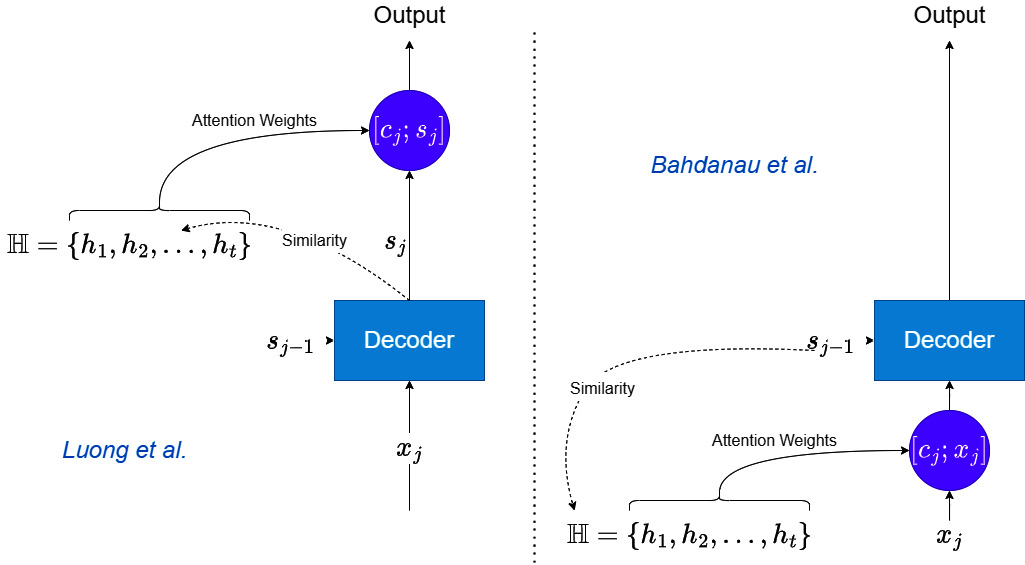
Figure 14.3 – Attention-based decoding: Bahdanau versus Luong

In our implementation, we have chosen the Bahdanau way of decoding, where we use the concatenated context vector and input as the input for decoding. And because of that, there is a condition the decoder must satisfy: the input_size parameter of the decoder should be equal to the sum of the input_size parameter of the encoder and the hidden_size parameter of the encoder. This validation is inbuilt into Seq2SeqwAttnConfig.

The following code block has all the code necessary for decoding with attention and has line numbers so that we can go line by line and explain what we are doing:

01        y_hat = torch.zeros_like(y, device=y.device)
02        dec_input = x[:, -1:, :]
03        for i in range(y.size(1)):
04            top_h = self._get_top_layer_hidden_state(h)
05            context = self.attention(
06                top_h.unsqueeze(1), o
07            )
08            dec_input = torch.cat((dec_input, context.unsqueeze(1)), dim=-1)
09            out, h = self.decoder(dec_input, h)
10            out = self.fc(out)
11            y_hat[:, i, :] = out.squeeze(1)
12            teacher_force = random.random() < self.hparams.teacher_forcing_ratio
13            if teacher_force:
14                dec_input = y[:, i, :].unsqueeze(1)
15            else:
16                dec_input = out

Lines 1 and 2 are the same as in the Seq2SeqModel class where we set up the variable to store the prediction and extract the starting input to be passed to the decoder, and line 3 starts the loop for decoding step by step.

Now, in each step, we need to use the hidden state from the previous timestep to calculate the context vector. If you remember the output shapes of an RNN (Chapter 12, Building Blocks of Deep Learning for Time Series), we know that it is (number of layers, batch size, hidden size). But we need our query hidden state to be of the dimension (batch size, hidden size). Luong et al. suggested using the hidden states from the top layer of a stacked RNN model as the query, and we are doing just that here:

hidden_state[-1, :, :]

If the RNN is bi-directional, we would need to slightly alter the retrieval because now, the last two rows of the tensor would be the output from the last layer (one forward and one backward). There are many ways we can combine these into a single tensor—we can concatenate them, we can sum them, or we can even mix them using a linear layer. Here, we just concatenate them:

torch.cat((hidden_state[-1, :, :], hidden_state[-2, :, :]), dim=-1)

And now that we have the hidden state, we use it as the query in the attention layer (line 5). In line 8, we concatenate the context with the input. Lines 9 to 16 do the rest of the decoding similar to Seq2SeqModel.

The notebook trains a multi-step Seq2Seq model (the best-performing variant with teacher forcing) with all the different types of attention we covered in the chapter using the same setup we developed in the last chapter. The results are summarized in the following table:

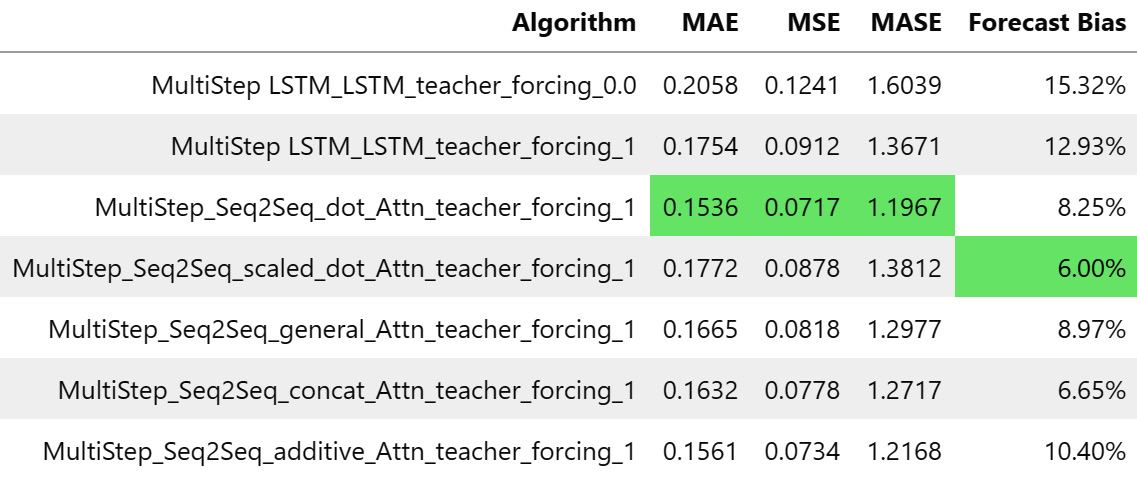
Figure 14.4 – Summary table for Seq2Seq models with attention

We can see that it is showing considerable improvements in MAE, MSE, and MASE by including attention, and out of all the variants of attention, the simple dot product attention performed the best, closely followed by additive attention. At this point, some of you might have a question in your mind—Why didn’t the scaled dot product work better than dot product attention? Scaling was supposed to make the dot product work better, wasn’t it?

There is a lesson to be learned here (which applies to all machine learning (ML)). No matter how much better a particular technique is in theory, you can always find examples in which it performs worse. And here, we saw just one household, and it is not surprising that we saw that scaled dot product attention didn’t work better than the normal dot product attention. But if we had evaluated at scale and realized that this is a pattern across multiple datasets, then it would be concerning.

So, we have seen that attention does make the models better. There was a lot of research done on using attention in various forms to enhance the performance of neural network (NN) models. Most of that research was carried out in natural language processing (NLP), specifically in language translation and language modeling. Soon, researchers stumbled upon a surprising result that changed the course of DL progress drastically.

Transformers – Attention is all you need

While the introduction of attention was a shot in the arm for RNNs and Seq2Seq models, they still had one problem. The RNNs were recurrent, and that meant it needed to process each word in a sentence in a sequential manner. And for popular Seq2Seq model applications such as language translation, it meant processing long sequences of words became really time-consuming. In short, it was difficult to scale them to a large corpus of data. In 2017, Vaswani et al. authored a seminal paper titled Attention Is All You Need. Just as the title of the paper implies, they explored an architecture that used attention (scaled dot product attention) and threw away recurrent networks altogether. And to the surprise of NLP researchers around the world, these models (which were dubbed Transformers) outperformed the then state-of-the-art Seq2Seq models in language translation.

This spurred a flurry of research activity around this new class of models, and pretty soon, in 2018, Devlin et al. from Google developed a bi-directional version of Transformers and trained the now famous language model, BERT (which stands for Bidirectional Encoder Representations from Transformers), and broke many state-of-the-art results across multiple tasks. This is considered to be the moment when Transformers as a model class really arrived. Fast-forward to 2022—Transformer models are ubiquitous. They are used in almost all tasks in NLP, and in many other sequence-based tasks such as time series forecasting, reinforcement learning (RL), and so on. They have also been successfully used in computer vision (CV) tasks as well.

There have been numerous modifications and adaptations to the vanilla Transformer model to make it more suitable for time series forecasting. But let’s understand the vanilla Transformer architecture that Vaswani et al. proposed in 2017 first.

Attention is all you need

The model Vaswani et al. proposed (hereby referred to as the vanilla Transformer) is also an encoder-decoder model, but both the encoder and decoder are non-recurrent. They are entirely comprised of attention mechanisms and feed-forward networks. Since the Transformer model was developed first for text sequences, let’s use the same example to understand and then adapt to the time series context.

There are a few key components of the model that need to be understood to put the whole thing together. Let’s take them one by one.

Self-attention

We saw how scaled dot product attention works earlier in this chapter (in the Alignment functions section), but there, we were calculating attention between the encoder and decoder hidden states. Self-attention is when we have an input sequence, and we calculate the attention scores between that input sequence itself. Intuitively, we can think of this operation as enhancing the contextual information and enabling the downstream components to use this enhanced information for further processing.

We saw the PyTorch implementation for encoder-decoder attention earlier, but that implementation was more aligned toward the step-by-step decoding of an RNN. Computing the attention scores for each query-key pair in one shot is something very simple to achieve using standard matrix multiplication and is essential to computing efficiency.

Notebook alert

To follow along with the complete code, use the notebook named 02-Self-Attention and Multi-Headed Attention.ipynb in the Chapter14 folder.

In NLP, it is standard practice to represent each word as a learnable vector called an embedding. This is because text or strings have no place in a mathematical model. For our example’s sake, let’s assume we use an embedding vector of size 512 for each word, and let’s assume that the attention mechanism has an internal dimension of 64. Let’s elucidate the attention mechanism using a sentence with 10 words.

After embedding, the sentence would be a tensor with dimensions (10, 512). We need to have three learnable weight matrices, , , and , to project the input embedding into the attention dimension (64). See Figure 14.5:

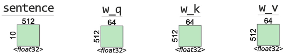
Figure 14.5 – Self-attention layer: input sentence and the learnable weights

The first operation projects the sentence tensor into a query, key, and value with dimensions equal to (sequence length, attention dim). This is done by using a matrix multiplication between the sentence tensor and learnable matrices. See Figure 14.6:

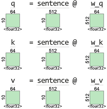
Figure 14.6 – Self-attention layer: query, key, and value projection

Now that we have the query, key, and value, we can calculate the attention weights of every query-key pair using matrix multiplication between the query and the transpose of the keys. The matrix multiplication is nothing but the dot product of each query with each of the values and gives us a square matrix of (sequence length, sequence length). See Figure 14.7:

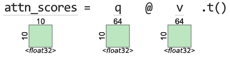
Figure 14.7 – Self-attention layer: attention scores between Q and K

Converting the attention scores to attention weights is just about scaling and applying the softmax function, as we discussed in the Scaled dot product attention section.

Now that we have the attention weights, we can use them to combine the value. The element-wise multiplication and then summing across the weights can be done efficiently using another matrix multiplication. See Figure 14.8:

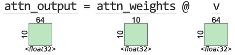
Figure 14.8 – Self-attention layer: combining V using the learned attention weights

Now, we have seen how attention is applied to all the query-key pairs in monolithic matrix operations rather than doing the same operation for each query in a sequential way. But Attention is All you Need proposed something even better.

Multi-headed attention

Since Transformers intended to take away the entire recurrent architecture, they needed to beef up the attention mechanism because that was the workhorse of the model. So, instead of using a single attention head, the authors of the paper proposed multiple attention heads acting together in different subspaces. We know that attention helps the model focus on a few elements from the many. Multi-headed attention (MHA) does the same thing but focuses on different aspects or different sets of elements, thereby increasing the capacity of the model. If we want to draw an analogy to the human mind, we consider many aspects of a situation before we take a decision.

For instance, if we decide to step out of the house, we will pay attention to the weather, we will pay attention to the time so that whatever we want to accomplish is still possible, we will pay attention to how punctual that friend you made a plan with has been in the past, and leave our house accordingly. Each of those aspects you can think of as one head of attention. Therefore, MHA enables Transformers to attend to multiple aspects at the same time.

Normally, if there are eight heads, we would assume that we would have to do the computation that we saw in the last section eight times. But thankfully, that is not the case. There are clever ways of accomplishing this MHA using the same kind of matrix multiplication, but now with larger matrices. Let’s see how that is done.

We will continue the same example and see a case where we have eight attention heads. There is one condition that needs to be satisfied to do this efficient calculation of MHA—the attention dimension should be divisible by the number of heads we are using.

The initial steps are exactly the same. We take in the input sentence tensor and project it into the query, key, and value. Now, we split the query, key, and value into separate query, key, and value subspaces for each head by doing some basic tensor re-arrangement. See Figure 14.9:

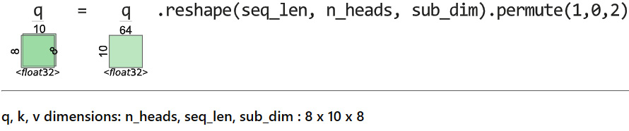
Figure 14.9 – Multi-headed attention: reshaping Q, K, and V into subspaces for each head

Now, we calculate the attention scores for each head in a single operation and combine them with the value to get the attention output for each head. See Figure 14.10:

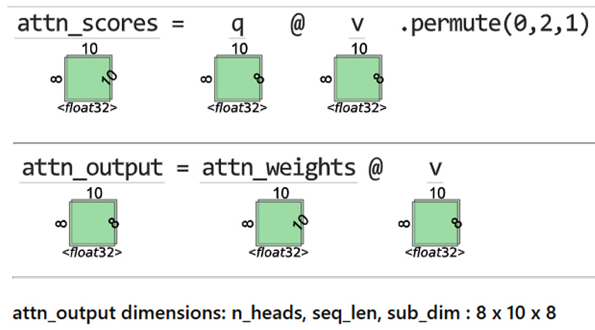
Figure 14.10 – Multi-headed attention: calculating attention weights and combining the value

We have the attention output of each head in the attn_output variable. Now, all we need to do is to reshape the array so that we stack the outputs from all the attention heads in a single dimension. See Figure 14.11:

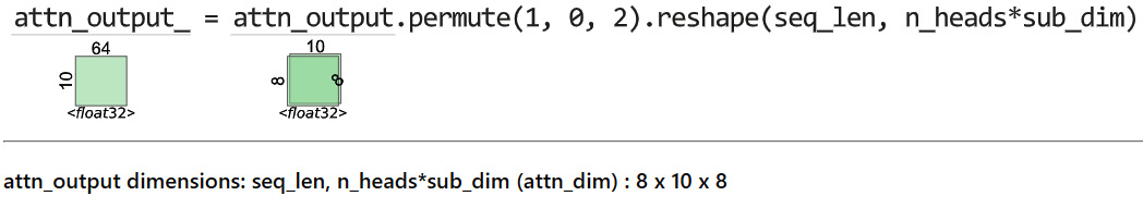
Figure 14.11 – Multi-headed attention: reshaping and stacking all the attention head outputs

In this way, we can do MHA in a fast and efficient manner. Now, let’s look at another key innovation that makes Transformers work.

Positional encoding

Transformers successfully avoided the recurrence and unlocked a performance bottleneck of sequential operations. But now there is a problem. By processing all the positions in a sequence in parallel, the model also loses the ability to understand the relevance of the position. For the Transformer, each position is independent of the other, and hence one key aspect we would seek from a model that processes sequences is missing. The original authors did propose a way to make sure we do not lose this information—positional encoding.

There have been many variants of positional encoding that have come up in subsequent years of research, but the most common one is still the variant that is used in the vanilla Transformer.

The solution proposed by Vaswani et al. was to add a particular vector, which encodes the position mathematically using sine and cosine functions, to each of the input tokens before processing them through the self-attention layer. If the input, is a -dimensional embedding for tokens in a sequence, positional embeddings, , is a matrix of the same size(). The element on the row and or column is defined as follows:

Although this looks a little complicated and counterintuitive, let’s break this down to understand it better.

From 20,000 feet, we know that these positional encodings capture the positional information, and we add them to the input embeddings. But why do we add them to the input embeddings? Let’s make that intuition clearer. Let’s assume the embedding dimension is just 2 (this is for ease of visualization and grabbing the concept better), and we have a word, A, represented using this token. For our experiment, let’s assume that we have the same word, A, repeated several times in our sequence. What happens if we add the positional encoding to it?

We know that the sine or cosine functions vary between 0 and 1. So, each of these encodings we add to the word embedding just perturbs the word embedding within a unit circle. As increases, we can see the position-encoded word embedding trace a unit circle around the original embedding (Figure 14.12):

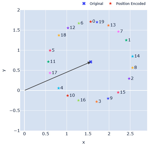
Figure 14.12 – Position encoding: intuition

In Figure 14.12, we have assumed a random embedding for a word, A (represented by the cross marker), and added position embedding assuming A is in different positions. And these position-encoded vectors are represented by star markers with the corresponding positions mentioned in numbers next to them. We can see how each position is a slightly perturbed point of the original vector, and it happens in a cyclical manner in a clockwise direction. We can see position 0 right at the top with 1, 2, 3, and so on in the clockwise direction. By having this representation, the model can figure out the word in different locations, and still retain the overall position in the semantic space.

Now that we know why we are adding the positional encodings to the input embeddings and have seen the intuition of why it works, let’s get down into more details and see how the terms inside the sine and cosine are calculated. represents the position of the token in the sequence. If the maximum length of the sequence is 128, varies from 0 to 127. represents the position along the embedding dimension, and because of the way the formula has been defined, for each value of , we have two values—a sine and a cosine. Therefore, will be half the number of dimensions, , and will go from 0 to .

With all this information, we know that the term inside the sine and cosine functions approaches 0 as we go toward the end of the embedding dimension. It also increases from 0 as we move along the sequence dimension. For each pair ( and ) of positions in the embedding dimension, we have a complementary sine and cosine wave, as Figure 14.13 shows:

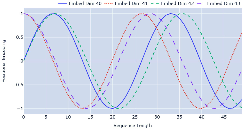
Figure 14.13 – Positional encoding: sine and cosine terms

We can see that embedding dimensions 40 and 41 are sine and cosine waves of the same frequency, and embedding dimensions 40 and 42 are sine waves with a slight increase in frequency. By using the combination of sine and cosine waves of varying frequencies, the positional encoding can encode rich positional information as a vector. If we plot a heatmap of the whole positional encoding vector (Figure 14.14), we can see how the values change and encode the positional information:

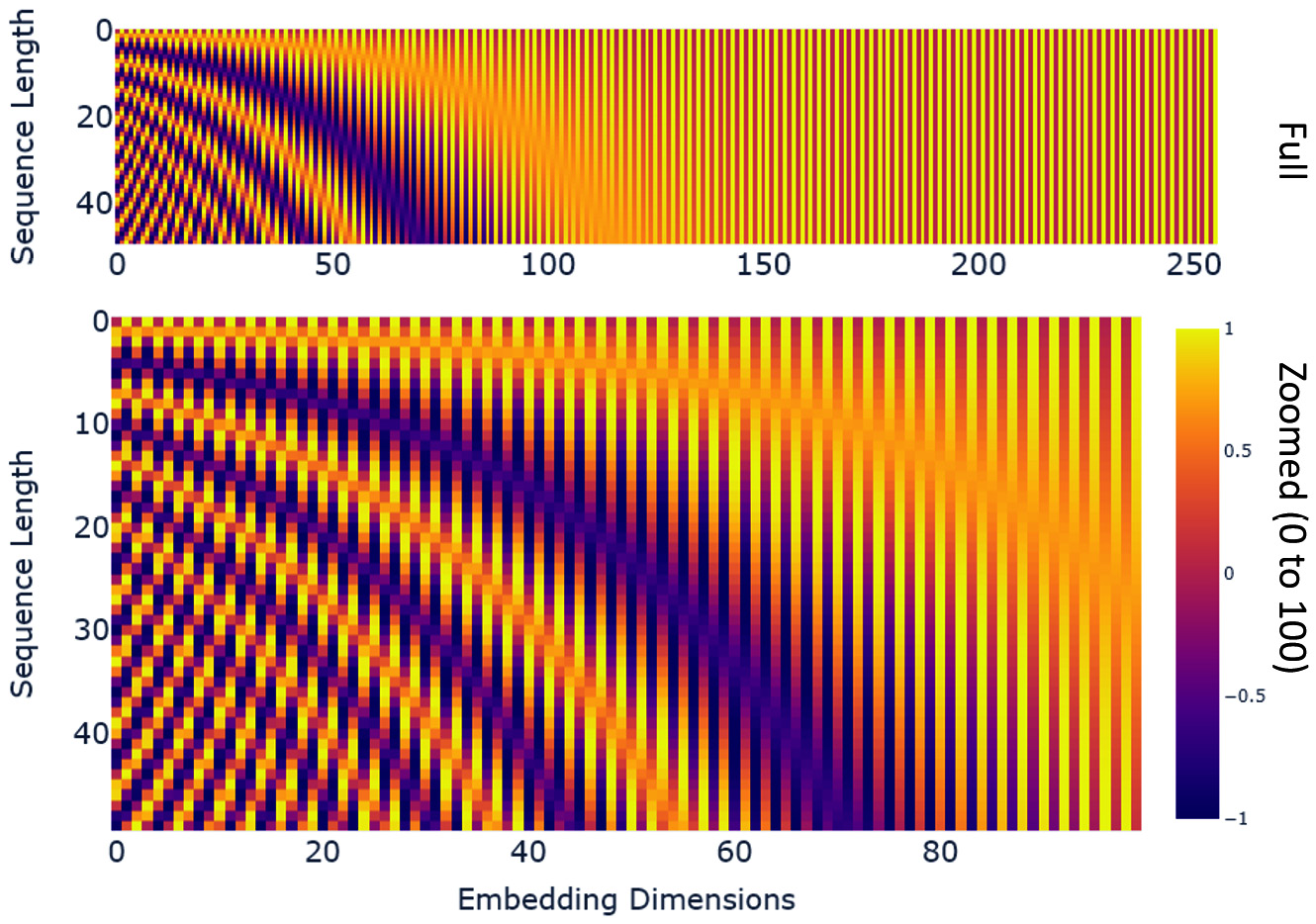
Figure 14.14 – Positional encoding: heatmap of the entire vector

Another interesting observation is that the positional encoding quickly shrinks to 0/1 as we move forward in the embedding dimension because the term inside the sine or cosine functions (angle in radians) quickly becomes zero on account of the large denominator. The zoomed plot shows the color differences more clearly.

Now for the last component in the Transformer model.

Position-wise feed-forward layer

We have already covered what feed-forward networks are in Chapter 12, Building Blocks of Deep Learning for Time Series. The only thing to be noted here is that the position-wise feed-forward layer is when we apply the same feed-forward layer in each position, independently. If we have 12 positions (or words), we will have a single feed-forward network to process each of these positions.

Vaswani et al. defined this as a two-layer feed-forward network where the transformations were defined in a way that the input dimensions get expanded to four times the input dimension, with a ReLU activation function applied at that stage, and then transformed back to the input dimension again. The exact operation can be written as a mathematical formula:

Here, is a matrix of dimensions (input size, 4*input size), is a matrix of dimensions (4*input size, input size), and are corresponding biases, and is the standard ReLU operator.

There have been studies where researchers have tried replacing ReLU with other activation functions, more specifically Gated Linear Units (GLUs), which have shown promise. Noam Shazeer from Google has a paper on the topic, and if you want to know more about these new activation functions, I recommend checking out his paper in the Further reading section.

Now that we know all the necessary components of a Transformer model, let’s see how they are put together.

Encoder

The vanilla Transformer model is an encoder-decoder model. There are N blocks of encoders, and each block contains an MHA layer and a position-wise feed-forward layer with residual connections in between (Figure 14.15):

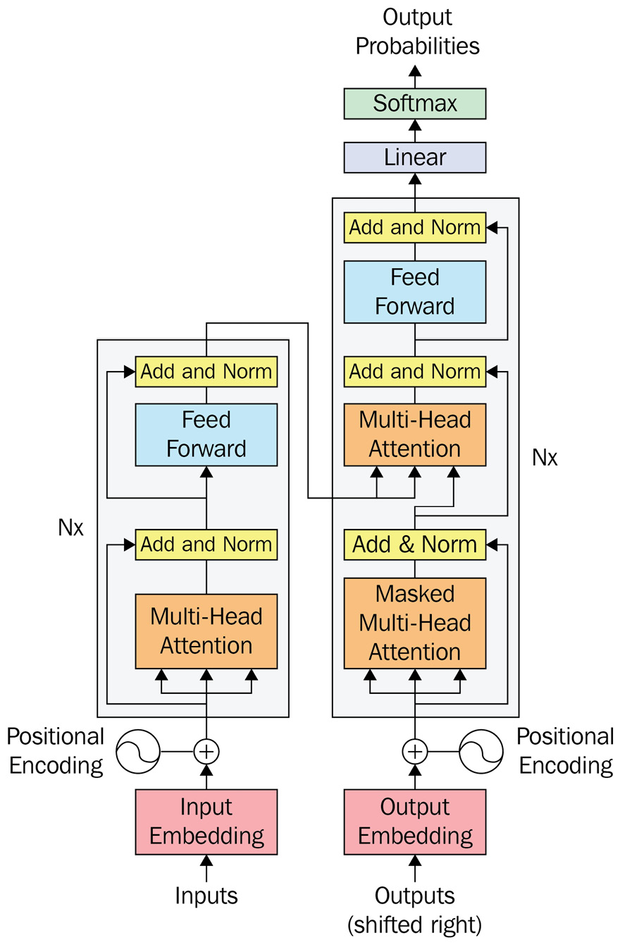
Figure 14.15 – Transformer model from Attention is All you Need by Vaswani et al.

For now, let’s focus on the left side of Figure 14.15, which is the encoder. The encoder takes in the input embeddings, with the positional encoding vector added to it, as the input. The three-pronged arrow that goes into MHA denotes the query, key, and value split. The output from the MHA goes into a block named Add & Norm. Let’s quickly see what that does.

There are two key operations that happen here—residual connections and layer normalization.

Residual connections

Residual connections (or skip connections) are a family of techniques that were introduced to DL to make learning deep networks easier. The primary benefit of the technique is that it makes the gradient flow through the network better and thereby encourages learning in all parts of the network. They incorporate a pass-through memory highway in the network. We have already seen one instance where a skip connection (although not an apparent one) resolved gradient flow issues—long short-term memory networks (LSTMs). The cell state in the LSTM serves as this highway to let gradients flow through the network without getting into vanishing gradient issues.

But nowadays, when we say residual connections, we typically think of ResNets, which made a splash in the history of DL through a convolutional NN (CNN) architecture that won major image classification challenges, including ImageNet in 2015. They introduced residual connections to train much deeper architectures than those prevalent at the time. The concept is deceptively simple. Let’s look at it visually:

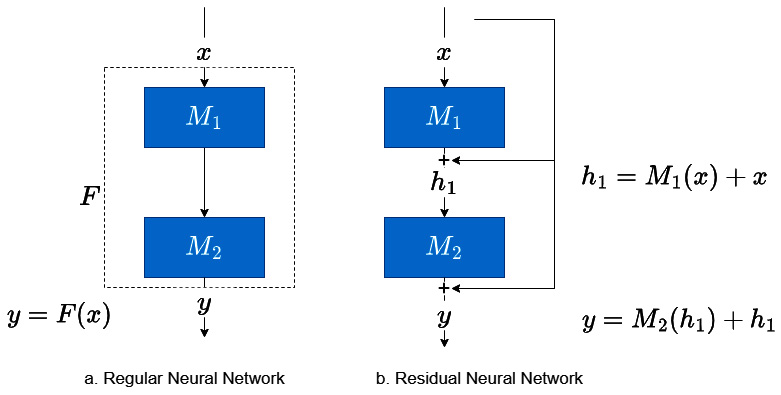
Figure 14.16 – Residual networks

Let’s assume a DL model with two layers with functions, and . In a regular NN, the input, , passes through the two layers to give us the output, . These two individual functions can be considered as a single function that converts to : .

In residual networks, we change this paradigm into saying that each individual function (or layer) only learns the difference between the input to the function and the expected output. That is where the name residual connections came from. So, if is the desired output and is the input, then . Rewriting that, we get . And this is what is most used as residual connections.

Among many benefits such as better gradient flows, residual connections also make the loss surface smooth (Li et al. 2018) and more amenable to gradient-based optimization. For more details and intuition around residual networks, I urge you to check out the blog linked in the Further reading section.

So, the Add in the Add & Norm block in the Transformer is actually the residual connection.

Layer normalization

Normalization in deep NNs (DNNs) has been an active field of research. Among many benefits, normalization leads to faster training, higher learning rates, and even a bit of regularization. Batch normalization is the most common normalization technique in use, typically in CV, which makes the input have approximately zero mean and unit variance by subtracting the input mean in the current batch and dividing it by the standard deviation.

But in NLP, researchers prefer layer normalization, where the normalization is happening across each feature. The difference can be seen in Figure 14.17:

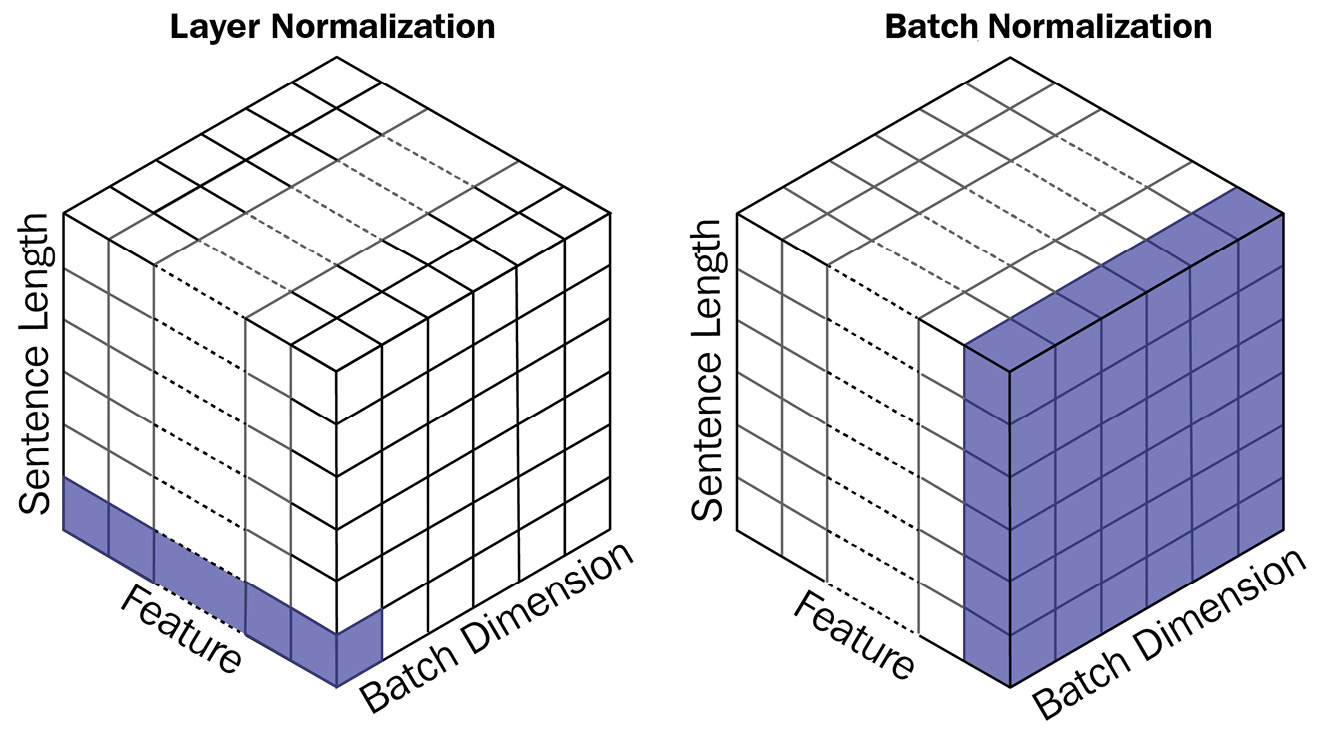
Figure 14.17 – Batch normalization versus layer normalization

This preference for layer normalization emerged empirically, but there have been studies and intuitions around the reason for this preference. NLP data usually has a higher variance as opposed to CV data, and this variance causes some problems for batch normalization. Layer normalization, on the other hand, is immune to this because it doesn’t rely on batch-level variance.

Either way, Vaswani et al. decided to use layer normalization in their Add & Norm block.

Now, we know the Add & Norm block is nothing but a residual connection that is then passed through a layer normalization. So, we can see that the position-encoded inputs are first used in the MHA layer, and the output from the MHA is added with the position-encoded inputs again and passed through a layer normalization. And now, this output is passed through the position-wise feed-forward network and another Add & Norm layer, and this becomes one block of the encoder. An important point to keep in mind is that the architecture of all the elements in the encoder is designed in such a way that the dimension of the input at each position is preserved throughout. In other words, if the embedding vector is of dimension 100, the output from the encoder will also have a dimension of 100. This is a convenient way to make it possible to have residual connections and stack as many layers on top of each other as possible. Now, there are multiple such encoder blocks stacked on top of each other to form the encoder of the Transformer.

Decoder

The decoder block is also very similar to the encoder block, but with one key addition. Instead of a single self-attention layer, the decoder block has a self-attention layer, which operates on the decoder input, and an encoder-decoder attention layer. The encoder-decoder attention layer takes the query from the decoder at each stage and the key and values from the top encoder block.

There is something peculiar to the self-attention that is applied in the decoder block. Let’s see what that is.

Masked self-attention

We talked about how the Transformer can process sequences in parallel and be computationally efficient. But the decoding paradigm poses another challenge. Suppose we have an input sequence, , and the task is to predict the next step. So, in the decoder, if we give the sequence, , because of the parallel-processing architecture, each sequence is processed at once using self-attention. And we know self-attention is agnostic to sequence order. If left unrestricted, the model will cheat by using information from the future timesteps to predict the current timestep. This is where masked attention becomes important.

We saw earlier in the Self-attention section how calculate a square matrix (if the query and key have the same length) of attention weights, and it is with these weights that we combine the information from the value vector. This self-attention has no concept of temporality, and all the tokens will attend to all other tokens irrespective of their position. Let’s see Figure 14.18 to solidify our intuition:

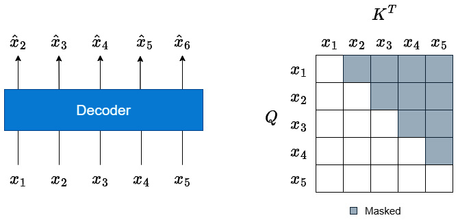
Figure 14.18 – Masked self-attention

We have the sequence, , and we are still trying to predict one step ahead. So, the expected output from the decoder would be . When we use self-attention, the attention weights that will be learned will be a square matrix of dimension. But if we look at the upper triangle of the square matrix (the part that is shaded in Figure 14.18), those combinations of tokens violate the temporal sanctity.

We can take care of this simply by adding a pre-generated mask that has zeros in all the white cells and -inf in all the shaded cells to the generated attention energies (the stage before applying softmax). This makes sure the attention weights for the shaded region will be zero, and this in turn ensures that no future information is used while calculating the weighted sum of the value vector.

Now, to wrap everything up, the output from the decoder is passed to a standard task-specific head to generate the output we desire.

We discussed the Transformer in the context of NLP, but it is a very small leap to adapt it to time series data.

Transformers in time series

Time series have a lot of similarities with NLP because of the fact that both deal with information in sequences. This can be further evidenced by the phenomenon that most of the popular techniques that are used in NLP are promptly adapted to a time series context. Transformers are no exception to that.

Instead of looking at tokens at each position, we have real numbers in each position. And instead of talking about input embeddings, we can talk in terms of input features. The vector of features at each timestep can be considered the equivalent of an embedding vector in NLP. And instead of making causal decoding an optional step (in NLP, that really depends on the task at hand), we have a strict requirement for causal decoding. There, it is trivial to adapt Transformers to time series, although in practice, there are many challenges because in time series we typically encounter sequences that are much longer than the ones in NLP, and this creates a problem because the complexity of self-attention is scaled quadratically with respect to the input sequence length. There have been many alternate proposals for self-attention that make it feasible to use it for long sequences as well, and we will be covering a few of them in Chapter 16, Specialized Deep Learning Architectures for Forecasting.

Now, let’s try to put everything we have learned about Transformers into practice.

Forecasting with Transformers

For some continuity, we will continue with the same household we were forecasting with RNNs and RNNs with attention.

Notebook alert

To follow along with the complete code, use the notebook named 03-Transformers.ipynb in the Chapter14 folder and the code in the src folder.

Although we learned about the vanilla Transformer as a model with an encoder-decoder architecture, it was really designed for language translation tasks. In language translation, the source sequence and target sequence are quite different, and therefore the encoder-decoder architecture made sense. But soon after, researchers figured out that using the decoder part of the Transformer alone does well. It is called a decoder-only Transformer in literature. The naming is a bit confusing because if you think about it, the decoder is different from the encoder in two things—masked self-attention and encoder-decoder attention. So, in a decoder-only Transformer, how do we have the encoder-decoder attention? The short answer is that we don’t. The architecture of the decoder-only Transformer resembles the encoder block more, but we call it decoder-only because we use masked self-attention to make our model respect the temporal sanctity of our sequences.

We are also going to implement a decoder-only Transformer. The first thing we need to do is to define a config class, TransformerConfig, with the following parameters:

• input_size—This parameter defines the number of features the Transformer is expecting.
• d_model—This parameter defines the hidden dimension of the Transformer or the dimension over which all the attention calculation and subsequent operations happen.
• n_heads—This parameter defines how many heads we have in the MHA mechanism.
• n_layers—This parameter defines how many blocks of encoders we are going to stack on top of each other.
• ff_multiplier—This parameter defines the scale of expansion within the position-wise feed-forward layers.
• activation—This parameter lets us define which activation we need to use in the position-wise feed-forward layers. It can be either relu or gelu.
• multi_step_horizon—This parameter lets us define how many timesteps into the future we should be forecasting.
• dropout—This parameter lets us define the magnitude of dropout regularization to be applied in the Transformer model.
• learning_rate—This defines the learning rate of the optimization procedure.
• optimizer_params, lr_scheduler, lr_scheduler_params—These are parameters that let us tweak the optimization procedure. Let’s not worry about these for now because all of them have been set to intelligent defaults.

Now, we are going to inherit the BaseModel class we defined in src/dl/models.py and define a TransformerModel class.

The first method we need to implement is _build_network. The entire model can be found in src/dl/models.py, but we will be covering the important aspects here as well.

The first module we need to define is a linear projection layer that takes in the input_size parameter and projects it into d_model:

self.input_projection = nn.Linear(
            self.hparams.input_size, self.hparams.d_model, bias=False
        )

This is an additional step we have introduced to adapt the Transformers to the time series forecasting paradigm. In the vanilla Transformer, this is not needed because each word is represented by an embedding vector that typically has dimensions such as 200 or 500. But while doing time series forecasting, we might have to do the forecasting with just one feature (which is the history), and this seriously restricts our ability to provide capacity to the model because, without the projection layer, d_model can only be equal to input_size. Therefore, we have introduced a linear projection layer that decouples the number of features available and d_model.

Now, we need to have a module that adds positional encoding. We have packaged the same code we saw earlier into a PyTorch module and added it to src/dl/models.py. We just use that module and define our positional encoding operator, like so:

self.pos_encoder = PositionalEncoding(self.hparams.d_model)

We said earlier that we are going to use a decoder-only approach to building the model, and for that, we are using the TransformerEncoderLayer and TransformerEncoder modules defined in PyTorch. Just keep in mind that when using these layers, we will be using masked self-attention, and that makes it a decoder-only Transformer. The code is presented here:

self.encoder_layer = nn.TransformerEncoderLayer(
            d_model=self.hparams.d_model,
            nhead=self.hparams.n_heads,
            dropout=self.hparams.dropout,
            dim_feedforward=self.hparams.d_model * self.hparams.ff_multiplier,
            activation=self.hparams.activation,
            batch_first=True,
        )
        self.transformer_encoder = nn.TransformerEncoder(
            self.encoder_layer, num_layers=self.hparams.n_layers
        )

The last module we need to define is a linear layer that converts the output from the Transformer into the number of timesteps we are forecasting:

self.decoder = nn.Sequential(nn.Linear(self.hparams.d_model, 100),
            nn.ReLU(),
            nn.Linear(100, self.hparams.multi_step_horizon)
        )

That concludes the definition of the model. Now, let’s define a forward pass in the forward method.

The first step is to generate a mask we need to apply masked self-attention:

mask = self._generate_square_subsequent_mask(x.shape[1]).to(x.device)

We define the mask to have the same length as the input sequence. _generate_square_subsequent_mask is a method we have defined that generates a mask. Assuming the sequence length is 5, we can look at the two steps in preparing the mask:

mask = (torch.triu(torch.ones(5, 5)) == 1).transpose(0, 1)

torch.ones(sz,sz) creates a square matrix with all ones, and torch.triu(torch.ones(sz,sz)) makes the matrix with a top triangle (including the diagonal) as ones and the rest as zeros. And by using an equality operator with one condition and transposing it, we get a mask that has True in all the bottom triangles, including the diagonal, and False everywhere else. The output of the previous statement will be this:

tensor([[ True, False, False, False, False],
        [ True,  True, False, False, False],
        [ True,  True,  True, False, False],
        [ True,  True,  True,  True, False],
        [ True,  True,  True,  True,  True]])

We can see that this matrix has False at all the places where we need to mask attention. Now, all we need to do is to fill all True instances with 0 and all False instances with -inf:

mask = (
                mask.float()
                .masked_fill(mask == 0, float("-inf"))
                .masked_fill(mask == 1, float(0.0))
            )

These two lines of code are packaged into the _generate_square_subsequent_mask method, which we can use while training the model.

Now that we have created the mask for masked self-attention, let’s start processing the input, x:

# Projecting input dimension to d_model
x_ = self.input_projection(x)
# Adding positional encoding
x_ = self.pos_encoder(x_)
# Encoding the input
x_ = self.transformer_encoder(x_, mask)
# Decoding the input
y_hat = self.decoder(x_)

In these four lines of code, we project the input to d_model dimensions, add positional encoding, pass it through the Transformer model, and lastly use the linear layer to convert the output to the predictions we want.

Now we have y_hat, which is the prediction from the model. All we need to think of now is how to train this output to be the desired output.

We know that the Transformer model processes all tokens in one shot, and if we have N elements in the sequence, we will have N predictions as well (each prediction corresponding to the next timestep). And if each prediction is of the next H timesteps, the shape of y_hat would be (B, N, H), where B is the batch size. There are a few ways we can use this output to compare with the target. The most simple and naïve way is to just take the prediction from the last position (which will have H timesteps) and compare it with y (which also has H timesteps).

But this is not the most efficient way of using all the information we have, is it? We are discarding N-1 predictions and not giving any signal to the model on all those N-1 predictions. So, while training, it makes sense to use all these N-1 predictions also so that the model has a much richer signal feeding back while learning.

We can do that by using the original input sequence, x, but offsetting it by one. When H=1, we can think of this as a simple task where each position’s prediction is compared with the target for the next position (one step ahead). We can easily accomplish this by concatenating x[:,1:,:] (the input sequence offset by 1) with y (the original target) and treating this as the target. But when H>1, this becomes slightly complicated, but we can still do it by using a helpful function from PyTorch called unfold:

y = torch.cat([x[:, 1:, :], y], dim=1).squeeze(-1).unfold(1, y.size(1), 1)

We first concatenate the input sequence (offset by one) with y and then use unfold to create siding windows of size=H. This gives us a target of the same shape, (B,N,H).

But during inference (when we are predicting using a trained model), we do not need the output of all the other positions, and hence we discard them, as seen here:

y_hat = y_hat[:, -1, :].unsqueeze(1)

Our BaseModel class that we defined also lets us define a slightly different prediction step by using a predict method. You can look over the complete model in src/dl/models.py once again to solidify your understanding now.

Now that we have defined the model, we can use the same framework we have been using to train TransformerModel. The full code is available in the notebook, but we will just look at a summary table with the results:

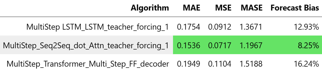
Figure 14.19 – Metrics for Transformer model on MAC000193 household

We can see that the model is not doing as well as its RNN cousins. There can be many reasons for this, but the most probable one is that Transformers are really data-hungry. Transformers have far fewer inductive biases and therefore only shine where there is lots of data available to learn from. When forecasting just one household alone, our model has access to far less data and may not work very well. This is true, to an extent, for all the DL models we have seen so far. In Chapter 10, Global Forecasting Models, we talked about how we can train a single model for multiple households together, but that discussion was limited to classical ML models. DL is also perfectly capable of global forecasting models and that is exactly what we will be talking about in the next chapter—Chapter 15, Strategies for Global Deep Learning Forecasting Models.

For now, congratulations on getting through another concept-heavy and information-packed chapter. The concept of attention, which has taken the field by storm, should be clearer in your mind now than when you started the chapter. I urge you to take a second stab at the chapter, read through the Further reading section, and do some of your own googling if it’s not clear because the future chapters assume you have this understanding.

Summary

We have been storming through the world of DL in the last few chapters. We started off with the basic premise of DL, what it is, and why it became so popular. Then, we saw a few common building blocks that are typically used in time series forecasting and got our hands dirty, learning how we can put what we have learned into practice using PyTorch. Although we talked about RNNs, LSTMs, GRUs, and so on, we purposefully left out attention and Transformers because they deserved a separate chapter.

We started the chapter by learning about the generalized attention model, helping you put a framework around all the different schemes of attention out there, and then went into detail on a few common attention schemes, such as scaled dot product, additive, and general attention. Right after incorporating attention into the Seq2Seq models we were playing with in Chapter 12, Building Blocks of Deep Learning for Time Series, we started with the Transformer. We went into detail on all the building blocks and architecture decisions involved in the original Transformer from the point of view of NLP, and after understanding the architecture, we adapted it to a time-series setting.

And finally, we capped it off by training a Transformer model for forecasting on a sample household. And now, by finishing this chapter, we have all the basic ingredients to really start using DL for time series forecasting.

In the next chapter, we are going to elevate what we have been doing and move on to the global forecasting model paradigm.

References

Following is the list of the references used in this chapter:

1. Dzmitry Bahdanau, KyungHyun Cho, and Yoshua Bengio (2015). Neural Machine Translation by Jointly Learning to Align and Translate. In 3rd International Conference on Learning Representations. https://arxiv.org/pdf/1409.0473.pdf
2. Thang Luong, Hieu Pham, and Christopher D. Manning (2015). Effective Approaches to Attention-based Neural Machine Translation. In Proceedings of the 2015 Conference on Empirical Methods in Natural Language Processing. https://aclanthology.org/D15-1166/
3. André F. T. Martins, Ramón Fernandez Astudillo (2016). From Softmax to Sparsemax: A Sparse Model of Attention and Multi-Label Classification. In Proceedings of the 33rd International Conference on Machine Learning. http://proceedings.mlr.press/v48/martins16.html
4. Ben Peters, Vlad Niculae, André F. T. Martins (2019). Sparse Sequence-to-Sequence Models. In Proceedings of the 57th Annual Meeting of the Association for Computational Linguistics. https://aclanthology.org/P19-1146/
5. Ashish Vaswani, Noam Shazeer, Niki Parmar, Jakob Uszkoreit, Llion Jones, Aidan N. Gomez, Lukasz Kaiser, and Illia Polosukhin (2017). Attention is All you Need. In Advances in Neural Information Processing Systems. https://papers.nips.cc/paper/2017/hash/3f5ee243547dee91fbd053c1c4a845aa-Abstract.html
6. Jacob Devlin, Ming-Wei Chang, Kenton Lee, and Kristina Toutanova (2019). BERT: Pre-training of Deep Bidirectional Transformers for Language Understanding. In Proceedings of the 2019 Conference of the North American Chapter of the Association for Computational Linguistics: Human Language Technologies, Volume 1 (Long and Short Papers). https://aclanthology.org/N19-1423/
7. Hao Li, Zheng Xu, Gavin Taylor, Christoph Studer, and Tom Goldstein (2018). Visualizing the Loss Landscape of Neural Nets. In Advances in Neural Information Processing Systems. https://proceedings.neurips.cc/paper/2018/file/a41b3bb3e6b050b6c9067c67f663b915-Paper.pdf
8. Sneha Chaudhari, Varun Mithal, Gungor Polatkan, and Rohan Ramanath (2021). An Attentive Survey of Attention Models. ACM Trans. Intell. Syst. Technol. 12, 5, Article 53 (October 2021). https://doi.org/10.1145/3465055

Further reading

Here are a few resources for further reading:

• The Illustrated Transformer by Jay Alammar: https://jalammar.github.io/illustrated-transformer/
• Transformer Networks: A mathematical explanation why scaling the dot products leads to more stable gradients: https://towardsdatascience.com/transformer-networks-a-mathematical-explanation-why-scaling-the-dot-products-leads-to-more-stable-414f87391500
• Why is Bahdanau’s attention sometimes called concat attention?: https://stats.stackexchange.com/a/524729
• Noam Shazeer (2020). GLU Variants Improve Transformer. arXiv preprint: Arxiv-2002.05202. https://arxiv.org/abs/2002.05202
• What is Residual Connection? by Wanshun Wong: https://towardsdatascience.com/what-is-residual-connection-efb07cab0d55
• Attn: Illustrated Attention by Raimi Karim: https://towardsdatascience.com/attn-illustrated-attention-5ec4ad276ee3