
12
Building Blocks of Deep Learning for Time Series
While we laid the foundations of deep learning in the previous chapter, it was very general. Deep learning is a vast field with applications in all possible domains, but the focus of this book is time series forecasting.
So, in this chapter, let’s strengthen the foundation by looking at a few building blocks of deep learning that are commonly used in time series forecasting. Even though the global machine learning models perform well in time series problems, some deep learning approaches have also shown good promise. They are a good addition to your toolset due to the flexibility they allow when modeling.
In this chapter, we will cover the following topics:
- Understanding the encoder-decoder paradigm
- Feed-forward networks
- Recurrent neural networks
- Long short-term memory (LSTM) networks
- Gated recurrent unit (GRU)
- Convolution networks
Technical requirements
You will need to set up the Anaconda environment following the instructions in the Preface of the book to get a working environment with all the packages and datasets required for the code in this book.
The associated code for this chapter can be found at https://github.com/PacktPublishing/Modern-Time-Series-Forecasting-with-Python-/tree/main/notebooks/Chapter12.
Understanding the encoder-decoder paradigm
In Chapter 5, Time Series Forecasting as Regression, we saw that machine learning is all about learning a function that maps our inputs to the desired output:

Adapting this to time series forecasting (considering univariate time series forecasting to keep it simple), we can rewrite it as follows:

Here, t is the current timestep and N is the total amount of history available at time t.
Deep learning, like any other machine learning approach, is tasked with learning this function, which maps history to the future. In Chapter 11, Introduction to Deep Learning, we saw how deep learning learns good features using representation learning and then uses the learned features to carry out the task at hand. This understanding can be further refined to the time series perspective by using the encoder-decoder paradigm.
Like everything in research, it is not entirely clear when and who proposed this idea of the encoder-decoder architecture. In 1997, Ramon Neco and Mikel Forcada proposed an architecture for machine translation that had ideas reminiscent of the encoder-decoder paradigm. In 2013, Nal Kalchbrenner and Phil Blunsom proposed an encoder-decoder model for machine translation, although they did not call it that. But it is when Ilya Sutskever et al. (2014) and Cho et al. (2014) proposed two new models for machine translation, which worked independently, that this idea took off. Cho et al. called it the encoder-decoder architecture, while Sutskever et al. called it the Seq2Seq architecture. The key innovation it drove was the ability to model variable-length inputs and outputs in an end-to-end fashion.
The research papers by Ramon Neco et al., Nal Kalchbrenner et al., Cho et al., and Ilya Sutskever et al. are cited in the References section as 1, 2, 3, and 4, respectively.
The idea is very straightforward, but before we get into that, we need to have a high-level understanding of latent spaces and feature/input spaces.
The feature space, or the input space, is the vector space where your data resides. If the data has 10 dimensions, then the input space is the 10-dimensional vector space. Latent space is an abstract vector space that encodes a meaningful internal representation of the feature space. To understand this, we can think about how we, as humans, recognize a tiger. We do not remember every minute detail of a tiger; we just have a general idea of what a tiger looks like and its prominent features, such as its stripes. It is a compressed understanding of this concept that helps our brain process and recognize a tiger faster.
Now that we have an idea about latent spaces, let’s see what an encoder-decoder architecture does.
An encoder-decoder architecture has two main parts – an encoder and a decoder:
- Encoder: The encoder takes in the input vector, x, and encodes it into a latent space. This encoded representation is called the latent vector, z.
- Decoder: The decoder takes in the latent vector, z, and decodes it into the kind of output we need (
 ).
).
The following diagram shows the encoder-decoder setup visually:
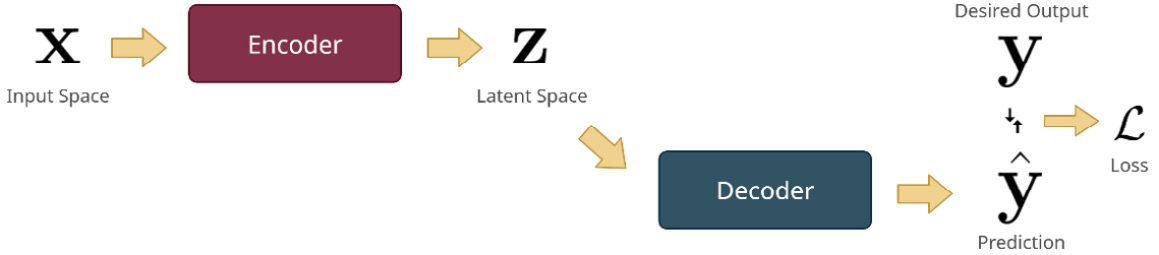
Figure 12.1 – The encoder-decoder architecture
In the context of time series forecasting, the encoder consumes the history and retains the information that is required for the decoder to generate the forecast. As we learned previously, time series forecasting can be written as follows:

Now, using the encoder-decoder paradigm, we can rewrite it as follows:


Here, h is the encoder and g is the decoder.
Each encoder and decoder can be some special architecture suited for time series forecasting. Let’s look at a few common components that are used in the encoder-decoder paradigm.
Feed-forward networks
Feed-forward networks (FFNs) or fully connected networks are the most basic architecture a neural network can take. We discussed perceptrons in Chapter 11, Introduction to Deep Learning. If we stack multiple perceptrons (both linear units and non-linear activations) and create a network of such units, we get what we call an FFN. The following diagram will help us understand this:
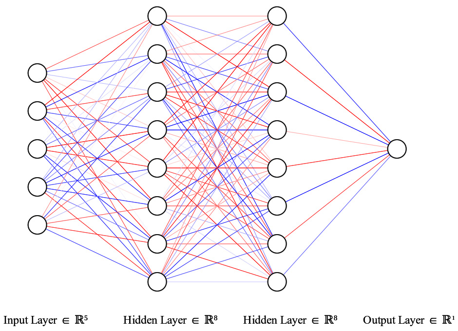
Figure 12.2 – Feed-forward network
An FFN takes a fixed-size input vector and passes it through a series of computational layers leading up to the desired output. This architecture is called feed-forward because the information is fed forward through the network. This is also called a fully connected network because every unit in a layer is connected to every unit in the previous layer and every unit in the next layer.
The first layer is called the input layer, and this is equal to the dimension of the input. The last layer is called the output layer, which is defined as per our desired output. If we need a single output, we will need one unit, while if we need 10 outputs, we will need 10 units. All the layers in between are called hidden layers. Two hyperparameters define the structure of the network – the number of hidden layers and the number of units in each layer. For instance, in Figure 12.2, we have a network with two hidden layers and eight units per layer.
In the time series forecasting context, an FFN can be used as an encoder as well as a decoder. As an encoder, we can use an FFN just like we used machine learning models in Chapter 5, Time Series Forecasting as Regression. We embed time and convert a time series problem into a regression problem before feeding it into the FFN. As a decoder, we use it on the latent vector (the output from the encoder) to get to the output (this is the most common usage of an FFN in time series forecasting).
Additional reading
We are going to be using PyTorch throughout this book to work with deep learning. If you are not comfortable with PyTorch, don’t worry – I’ll try and explain the concepts when necessary. To get a head start, you can go through the 01-PyTorch Basics.ipynb notebook in Chapter12, where we have explored the basic functionalities of tensors and trained a very small neural network from scratch using PyTorch. I also suggest heading over to the Further reading section at the end of this chapter, where you’ll find a few resources to learn PyTorch.
Now, let’s put on our practical hats and see some of these in action. PyTorch is an open source deep learning framework developed primarily by the Facebook AI Research Lab (FAIR). Although it is a library that can manipulate tensors (which are n-dimensional matrices) and accelerate such manipulations with a GPU, a large part of the use case for such a library is in building and training deep learning systems. Because of that, PyTorch provides a lot of ready-to-use components that we can use to build a deep learning system. Let’s see how we can use PyTorch for an FFN.
Notebook alert
To follow along with the complete code, use the 02-Building Blocks.ipynb notebook in the Chapter12 folder and the code in the src folder.
As we learned earlier in the section, an FFN is a network of linear and non-linear units arranged in a network. A linear operation consists of multiplying the input vector, ![]() , with a weight matrix,
, with a weight matrix, ![]() , and adding a bias term, b. This operation,
, and adding a bias term, b. This operation, ![]() , is encapsulated in a Linear class in the nn module of the PyTorch library. We can import this from the library using torch.nn import Linear. But usually, we must import the nn module as a whole because we would be using a lot of components from that module. For non-linearity, let’s use ReLU (as introduced in Chapter 11, Introduction to Deep Learning), which is also a class in the nn module.
, is encapsulated in a Linear class in the nn module of the PyTorch library. We can import this from the library using torch.nn import Linear. But usually, we must import the nn module as a whole because we would be using a lot of components from that module. For non-linearity, let’s use ReLU (as introduced in Chapter 11, Introduction to Deep Learning), which is also a class in the nn module.
Before moving on, let’s create a random walk time series whose length is 20:
N = 20
df = pd.DataFrame({
    "date": pd.date_range(periods=N, start="2021-04-12", freq="D"),
    "ts": np.random.randn(N)
})
We can use this tensor directly in the FFN, but usually, we use a sliding window technique to split the tensor and train the networks. We do this for multiple reasons:
- We can see this as a data augmentation technique that is creating a greater number of samples as opposed to using the entire sequence just once.
- It helps us reduce and restrict computation by limiting the calculation to a fixed window.
Let’s do that now:
ts = torch.from_numpy(df.ts.values).float()
window = 15
# Creating windows of 15 over the dataset
ts_dataset = ts.unfold(0, size=window, step=1)
Now, we have a tensor, ts_dataset, whose size is 6x15 (this can create 6 samples of 15 input features each when we move the sliding window across the length of the series). For a standard FFN, the input shape is specified as batch size x input features. So, 6 becomes our batch size and 15 becomes the input feature size.
Now, let’s define the layers in the FFN. For this exercise, let’s assume the network’s structure is as follows:
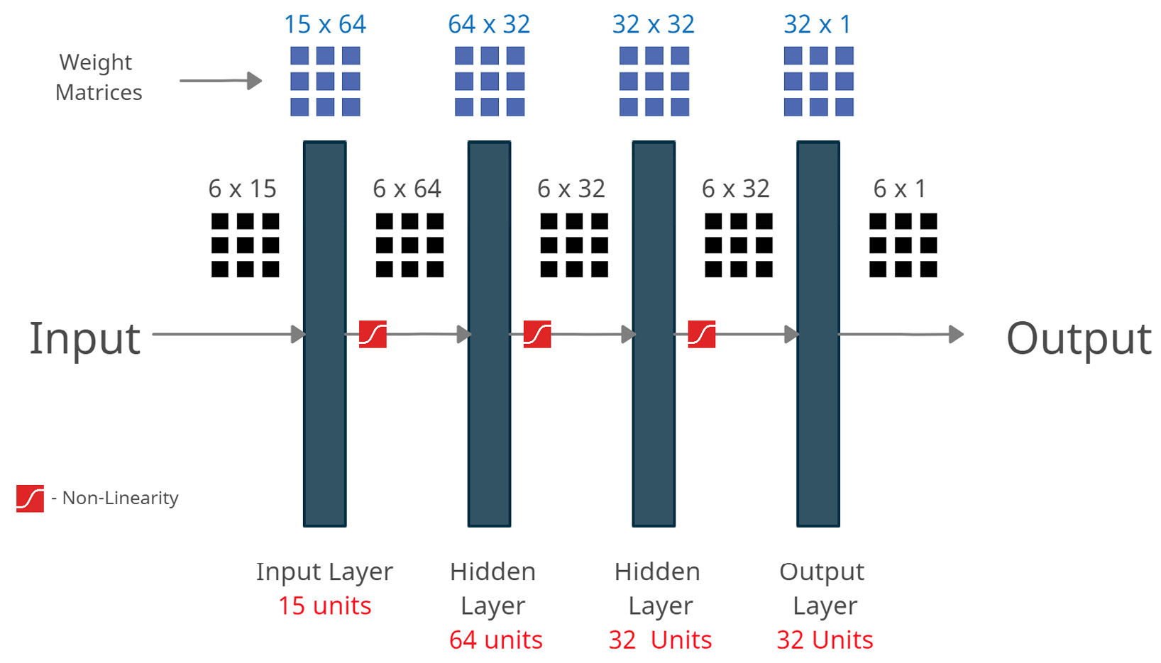
Figure 12.3 – FFNs – a matrix multiplication perspective
The input data (6x15) will be passed through these layers one by one. Here, we can see how the tensor dimensions are changing as it flows through the network. Each of the linear layers is essentially a matrix multiplication that converts the input into the output of a specified dimension. After each linear transformation, we stack a non-linear activation function in there. These alternative linear and non-linear modules are what give the neural network the expressive power it has. The linear layers are an affine transformation of the vector space (rotation, translation, and so on), and the non-linearity squashes the vector space. Together, they can morph the input space so that it’s useful for the task at hand. Now, let’s see how we can code this in PyTorch. We are going to use a handy module from PyTorch called Sequential, which allows us to stack different sub-components together and use them with ease:
# The FFN we define would have this architecture
# window(windowed input) >> 64 (hidden layer 1) >> 32 (hidden layer 2) >> 32 (hidden layer 2) >> 1 (output)
ffn = nn.Sequential(
    nn.Linear(in_features=window,out_features=64), # (batch-size x window) --> (batch-size x 64)
    nn.ReLU(),
    nn.Linear(in_features=64,out_features=32), # (batch-size x 64) --> (batch-size x 32)
    nn.ReLU(),
    nn.Linear(in_features=32,out_features=32), # (batch-size x 32) --> (batch-size x 32)
    nn.ReLU(),
    nn.Linear(in_features=32,out_features=1), # (batch-size x 32) --> (batch-size x 1)
)
Now that we have defined the FFN, let’s see how we can use it:
ffn(ts_dataset)
# or more explicitly
ffn.forward(ts_dataset)
This will return a tensor whose shape is based on batch size x output units. We can have any number of output units, not just one. Therefore, when using an encoder, we can have an arbitrary dimension for the latent vector. Then, when we are using it as a decoder, we can have the output units equal the number of time steps we are forecasting.
Sneak peek
We have not seen multi-step forecasting until now because it will be covered in more detail in Part 4, Mechanics of Forecasting. But for now, just understand that there are cases where we will need to forecast multiple time steps into the future. The classical statistical models do this out of the box. But for machine learning and deep learning, we need to design systems that can do that. Fortunately, there are a few different techniques to do so which will be covered in Part 4 of the book.
FFNs are designed for non-temporal data. We can use FFNs by embedding our data temporally and then passing that to the network. Also, the computational cost in an FFN is directly proportional to the memory we use in the embedding (the number of previous time steps we include as features). We will also not be able to handle variable-length sequences in this setting.
Now, let’s look at another common architecture that is specifically designed for temporal data.
Recurrent neural networks
Recurrent neural networks (RNNs) are a family of neural networks specifically designed to handle sequential data. They were first proposed by Rumelhart et al. (1986) in their seminal work, Learning Representations by Back-Propagating Errors. The work borrows ideas such as parameter sharing and recurrence from previous work in statistics and machine learning to come up with a neural network architecture that helps overcome many of the disadvantages FFNs have when processing sequential data.
Parameter sharing is when we use the same set of parameters for different parts of the model. Apart from a regularization effect (restricting the model to using the same set of weights for multiple tasks, which regularizes the model by constraining the search space while optimizing the model), parameter sharing enables us to extend and apply the model to examples of different forms. RNNs can scale to much longer sequences because of this. In an FFN, each timestep (each feature) has a fixed weight and even if the motif we are looking for shifts by one timestep, the network may not capture it correctly. In an RNN enabled by parameter sharing, they are captured in a much better way.
In sentences (which are also sequences), we want the model to recognize that “Tomorrow I will go to the bank” and “I will go to the bank tomorrow” are the same thing. An FFN can’t do this, but an RNN will be able to because it uses the same parameters at all positions and will be able to identify the motif “I will go to the bank” wherever it occurs. Intuitively, we can think of RNNs as applying the same FFN at each time window but enhanced with some kind of memory to store relevant information for the task at hand.
Let’s visualize how an RNN processes inputs:
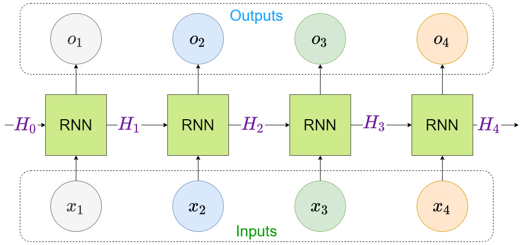
Figure 12.4 – How an RNN processes input sequences
Let’s assume we are talking about a sequence with four elements in it, ![]() . Any RNN block (let’s consider it as a black box for now) consumes input and a hidden state (memory) and produces an output. In the beginning, there is no memory, so we start with an initial memory (
. Any RNN block (let’s consider it as a black box for now) consumes input and a hidden state (memory) and produces an output. In the beginning, there is no memory, so we start with an initial memory (![]() ), which is typically an array filled with zeroes. Now, the RNN block takes in the first input (
), which is typically an array filled with zeroes. Now, the RNN block takes in the first input (![]() ) along with the initial hidden state (
) along with the initial hidden state (![]() ) and produces an output (
) and produces an output (![]() ) and a hidden state (
) and a hidden state (![]() ).
).
To process the second element in the sequence, the same RNN block takes in the hidden state from the previous timestep (![]() ) and the input at the current timestep (
) and the input at the current timestep (![]() ) to produce the output at the second timestep (
) to produce the output at the second timestep (![]() ) and a new hidden state (
) and a new hidden state (![]() ). This process continues until we reach the end of the sequence. After processing the entire sequence, we will have all the outputs at each timestep (
). This process continues until we reach the end of the sequence. After processing the entire sequence, we will have all the outputs at each timestep (![]() ) and the final hidden state (
) and the final hidden state (![]() ).
).
These outputs and the hidden state will have encoded the information contained in the sequence and can be used for further processing, such as to predict the next step using a decoder. The RNN block can also be used as a decoder that takes in the encoded representation and produces the outputs. Because of this flexibility, the RNN blocks can be arranged to suit a wide variety of input and output combinations, such as the following:
- Many-to-one, where we have many inputs and a single output – for instance, single-step forecasting or time series classification
- Many-to-many, where we have many inputs and many outputs – for instance, multi-step forecasting
Now let’s look at what happens inside an RNN.
Let the input to the RNN at time ![]() be
be ![]() , and the hidden state from the previous timestep be
, and the hidden state from the previous timestep be ![]() . The updated equations are as follows:
. The updated equations are as follows:
Here, U, V, and W are learnable weight matrices and ![]() and
and ![]() are two learnable bias vectors. U, V, and W can be easily remembered as input-to-hidden, hidden-to-output, and hidden-to-hidden matrices based on the kind of transformation they perform, respectively. Intuitively, we can think of the operation that the RNN is doing as a kind of learning and forgetting the information as it sees fit. The tanh activation, as we saw in Chapter 11, Introduction to Deep Learning, produces a value between -1 and 1, which acts analogous to forgetting and remembering. So, the RNN transforms the input into a latent dimension, uses the tanh activation to decide what information from the current timestep and previous memory to keep and forget, and uses this new memory to generate an output.
are two learnable bias vectors. U, V, and W can be easily remembered as input-to-hidden, hidden-to-output, and hidden-to-hidden matrices based on the kind of transformation they perform, respectively. Intuitively, we can think of the operation that the RNN is doing as a kind of learning and forgetting the information as it sees fit. The tanh activation, as we saw in Chapter 11, Introduction to Deep Learning, produces a value between -1 and 1, which acts analogous to forgetting and remembering. So, the RNN transforms the input into a latent dimension, uses the tanh activation to decide what information from the current timestep and previous memory to keep and forget, and uses this new memory to generate an output.
In standard backpropagation, we backpropagate the gradients from one unit to another. But in recurrent nets, we have a special situation where we have to backpropagate the gradients within a single unit, but through time or the different time steps. A special case of backpropagation, called Back Propagation Through Time (BPTT), has been developed for RNNs. Thankfully, all the major deep learning frameworks are capable of doing this without any problems. For a more detailed understanding and mathematical foundations of BPTT, please to the Further reading section.
PyTorch has made RNNs available as ready-to-use modules – all you need to do is import one of the modules from the library and start using it. But before we do that, we need to understand a few more concepts.
The first concept we will look at is the possibility of stacking multiple layers of RNNs on top of each other so that the outputs at each timestep become the input to the RNN in the next layer. Each layer will have a hidden state or memory. This enables hierarchical feature learning, which is one of the bedrocks of the successes of deep learning today.
Another concept is bidirectional RNNs, introduced by Schuster and Paliwal in 1997. Bidirectional RNNs are very similar to RNNs. In a vanilla RNN, we process the inputs sequentially from start to end (forward). However, a bidirectional RNN uses one set of input-to-hidden and hidden-to-hidden weights to process the inputs from start to end and another set to process the inputs in reverse (end to start) and concatenate the hidden states from both directions. It is on this concatenated hidden state that we apply the output equation.
Reference check
The research papers by Rumelhart et al and Schuster and Paliwal are cited in the References section as 5 and 6, respectively.
The RNN layer in PyTorch
Now, let’s understand the PyTorch implementation for RNN. As with the Linear module, the RNN module is also available from torch.nn. Let’s look at the different parameters the implementation provides while initializing:
- input_size: The number of expected features in the input. If we are using just the history of the time series, then this would be 1. However, when we use history along with some other features, then this will be >1.
- hidden_size: The dimension of the hidden state. This defines the size of the input-to-hidden and hidden-to-hidden matrices.
- num_layers: This is the number of RNNs that will be stacked on top of each other. The default is 1.
- nonlinearity: The non-linearity to use. Although tanh is the originally proposed non-linearity, PyTorch also allows us to use ReLU (relu). The default is ‘tanh’.
- bias This parameter decides whether or not to add bias to the update equations we discussed earlier. If the parameter is False, there will be no bias. The default is True.
- batch_first: There are two input data configurations that the RNN cell can use – we can have the input as (batch size, sequence length, number of features) or (sequence length, batch size, number of features). batch_first = True selects the former as the expected input dimensions. The default is False.
- dropout: This parameter, if non-zero, uses a dropout layer on the outputs of each RNN layer except the last. Dropout is a popular regularization technique where randomly selected neurons are ignored during training (the Further reading section contains a link to the paper that proposed this). The dropout probability will be equal to dropout. The default is 0.
- bidirectional: This parameter enables a bidirectional RNN. If True, a bidirectional RNN is used. The default is False.
To continue applying the model to the same synthetic data we generated earlier in this chapter, let’s initialize the RNN model, as follows:
rnn = nn.RNN(
    input_size=1,
    hidden_size=32,
    num_layers=1,
    batch_first=True,
    dropout=0,
    bidirectional=False,
)
Now, let’s look at the inputs and outputs that are expected from an RNN cell.
As opposed to the Linear layer we saw earlier, the RNN cell takes in two inputs – the input sequence and the hidden state vector. The input sequence can be either (batch size, sequence length, number of features) or (sequence length, batch size, number of features), depending on whether we have set batch_first=True. The hidden state is a tensor whose size is (D*number of layers, batch size, hidden size), where D = 1 for bidirectional=False and D = 2 for bidirectional=True. The hidden state is an optional input and will default to zero tensors if left blank.
There are two outputs of the RNN cell: an output and a hidden state. The output can be either (batch size, sequence length, D*hidden size) or (sequence length, batch size, D*hidden size), depending on batch_first. The hidden state has the dimension of (D*number of layers, batch size, hidden size). Here, D = 1 or 2 is based on the bidirectional parameter.
So, let’s run our sequence through an RNN and look at the inputs and outputs (for more detailed steps, refer to the accompanying notebook):
#input dim: torch.Size([6, 15, 1])
# batch size = 6, sequence length = 15 and number of features = 1, batch_first = True
output, hidden_states = rnn(rnn_input)
# output.shape -> torch.Size([6, 15, 32])
# hidden_states.shape -> torch.Size([1, 6, 32]))
Important note
Although we saw that the RNN cell contains the output as well as the hidden state, we also know that the output is just an affine transformation of the hidden state. Therefore, to provide flexibility to the users, PyTorch only implements the update equations regarding the hidden states in the module. There are cases where we have no use for the outputs at each timestep (such as in a many-to-one scenario) and we can save computation if we do not do the output update at each step. Therefore, output from the PyTorch RNN is just the hidden states at each timestep and hidden_states is the latest hidden state.
We can verify this by checking whether the hidden state tensor is equal to the last output tensor:
torch.equal(hidden_states[0], output[:,-1]) # -> True
To make this clearer, let’s look at it visually:
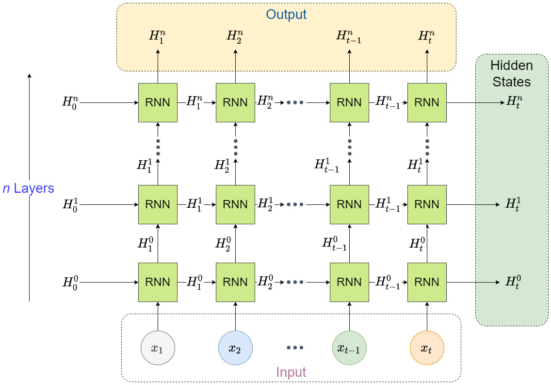
Figure 12.5 – PyTorch implementation of stacked RNNs
The hidden states at each timestep are used as input for the subsequent layer of RNNs and the hidden states of the last layer of RNNs are collected as the output. But each layer has a hidden state (that’s not shared with the others) and the PyTorch RNN collects the last hidden state from each layer and gives us that as well. Now, it is up to us to decide how to use these outputs. For instance, in a one-step-ahead forecast, we can use the output hidden states and stack a few linear layers on top of it to get the next timestep prediction. Alternatively, we can use the hidden states to transfer memory into another RNN as a decoder and generate predictions for multiple time steps. There are many more ways we can use this output and PyTorch gives us that flexibility.
RNNs, while very effective in modeling sequences, have one big flaw. Because of BPTT, the number of units through which you need to backpropagate increases drastically with the length of the sequence to be used for training. When we have to backpropagate through such a long computational graph, we will encounter vanishing or exploding gradients. This is when the gradient, as it is backpropagated through the network, either shrinks to zero or explodes to a very high number. The former makes the network stop learning, while the latter makes the learning unstable.
We can think of what’s happening as akin to what happens when we multiply a scalar number repeatedly by itself. If the number is less than one, with every subsequent multiplication, the number becomes smaller and smaller until it is practically zero. If the number is greater than one, then the number becomes larger and larger at an exponential scale. This was discovered, independently, by Hochreiter in his diploma thesis (1991) and Yoshua Bengio et al. in two papers published in 1993 and 1994. Over the years, many tweaks to the model and training process have been proposed to tackle this disadvantage. Nowadays, vanilla RNNs are hardly used in practice and have been replaced almost completely by their newer cousins.
Reference check
The references for Hochreiter (1991) and Bengio et al. (1993, 1994) are cited in the References section as 7, 8, and 9, respectively.
Now, let’s look at two key improvements that have been made to the RNN architecture that have shown good performance and gained popularity in the machine learning community.
Long short-term memory (LSTM) networks
Hochreiter and Schmidhuber proposed a modification of the classical RNNs in 1997 – LSTM networks. It aimed to resolve the vanishing and exploding gradients in vanilla RNNs. The design of the LSTM was inspired by the logic gates of a computer. It introduces a new component, called a memory cell, which serves as long-term memory and is used in addition to the hidden state memory of classical RNNs. In an LSTM, multiple gates are tasked with reading, adding, and forgetting information from these memory cells. This memory cell acts as a gradient highway, allowing the gateways to pass relatively unhindered through the network. This is the key innovation that avoided vanishing gradients in RNNs.
Let the input to the LSTM at time ![]() be
be ![]() , and the hidden state from the previous timestep be
, and the hidden state from the previous timestep be ![]() . Now, there are three gates that process information. Each gate is nothing but two learnable weight matrices (one for the input and one for the hidden state from the last step) and a bias term that is multiplied/added to the input and hidden state and finally passed through a sigmoid activation. The output of these gates will be a real number between 0 and 1. Let’s look at each of these gates in detail:
. Now, there are three gates that process information. Each gate is nothing but two learnable weight matrices (one for the input and one for the hidden state from the last step) and a bias term that is multiplied/added to the input and hidden state and finally passed through a sigmoid activation. The output of these gates will be a real number between 0 and 1. Let’s look at each of these gates in detail:
- Input gate: The function of this gate is to decide how much information to read from the current input and previous hidden state. The update equation for this is:

- Forget gate: The forget gate decides how much information to forget from long-term memory. The updated equation for this is:

- Output gate: The output gate decides how much of the current cell state should be used to create the current hidden state, which is the output of the cell. The update equation for this is:

Here, ![]() are learnable weight parameters and
are learnable weight parameters and  are learnable bias parameters.
Now, we can introduce a new long-term memory (cell state), ![]() . The three gates mentioned previously serve to update and forget from this memory. If the cell state from the previous timestep is
. The three gates mentioned previously serve to update and forget from this memory. If the cell state from the previous timestep is ![]() , then the LSTM cell calculates a candidate cell state,
, then the LSTM cell calculates a candidate cell state, ![]() , using another gate, but this time with tanh activation:
, using another gate, but this time with tanh activation:

Here, ![]() are learnable weight parameters and
are learnable weight parameters and ![]() is the learnable bias parameter.
is the learnable bias parameter.
Now, let’s look at the key update equation, which updates the cell state or long-term memory of the cell:
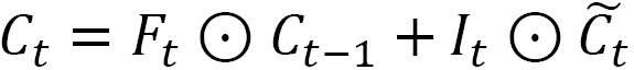
Here, ![]() is elementwise multiplication. Here, we use the forget gate to decide how much information from the previous timestep to carry forward, and the input gate to decide how much of the current candidate cell state will be written into long-term memory.
is elementwise multiplication. Here, we use the forget gate to decide how much information from the previous timestep to carry forward, and the input gate to decide how much of the current candidate cell state will be written into long-term memory.
Last but not least, we use the newly created current cell state and the output gate to decide how much information to pass on to the predictor through the current hidden state:

A visual representation of this process can be seen in Figure 12.6.
The LSTM layer in PyTorch
Now, let’s understand the PyTorch implementation of LSTM. It is very similar to the RNN implementation we saw earlier, but it has one key difference: the parameters to initialize the class are pretty much the same. The API for this can be found at https://pytorch.org/docs/stable/generated/torch.nn.LSTM.html#torch.nn.LSTM. The key difference here is how the hidden states are used. While the RNN has a single tensor as a hidden state, the LSTM expects a tuple of tensors of the same dimensions: (hidden state, cell state). LSTMs, just like RNNs, have stacked and bidirectional variants, and PyTorch handles them in the same way.
Now, let’s initialize some LSTM modules and use the synthetic data we have been using to see them in action:
lstm = nn.LSTM(
    input_size=1,
    hidden_size=32,
    num_layers=5,
    batch_first=True,
    dropout=0,
    # bidirectional=True,
)
output, (hidden_states, cell_states) = lstm(rnn_input)
output.shape # -> [6, 15, 32]
hidden_states.shape # -> [5, 6, 32]
cell_states.shape # -> [5, 6, 32]
Now, let’s look at another modification that’s been made to vanilla RNNs that has resolved the vanishing and exploding gradient problems.
Gated recurrent unit (GRU)
In 2014, Cho et al. proposed another variant of the RNN that has a much simpler structure than an LSTM, called a gated recurrent unit (GRU). The intuition behind this is similar to when we use a bunch of gates to regulate the information that flows through the cell, but a GRU eliminates the long-term memory component and uses just the hidden state to propagate information. So, instead of the memory cell becoming the gradient highway, the hidden state itself becomes the “gradient highway.” In keeping with the same notation convention we used in the previous section, let’s look at the updated equations for a GRU.
While we had three gates in an LSTM, we only have two in a GRU:
- Reset gate: This gate decides how much of the previous hidden state will be considered as the candidate's hidden state of the current timestep. The equation for this is:

- Update gate: The update gate decides how much of the previous hidden state should be carried forward and how much of the current candidate’s hidden state will be written into the hidden state. The equation for this is:

Here ![]() are learnable weight parameters and
are learnable weight parameters and ![]() are learnable bias parameters.
are learnable bias parameters.
Now, we can calculate the candidate’s hidden state (![]() ) as follows:
) as follows:

Here, ![]() are learnable weight parameters and
are learnable weight parameters and ![]() is the learnable bias parameter. Here, we use the reset gate to throttle the information flow from the previous hidden state to the current candidate’s hidden state.
is the learnable bias parameter. Here, we use the reset gate to throttle the information flow from the previous hidden state to the current candidate’s hidden state.
Finally, the current hidden state (the output that goes to a predictor) is computed using the following equation:

We use the update gate to decide how much from the previous hidden state and how much from the current candidate will be passed to the next timestep or predictor.
Reference check
The research papers for LSTM and GRUs are cited in the References section as 10 and 11, respectively.
A visual representation of this process can be found in Figure 12.6:
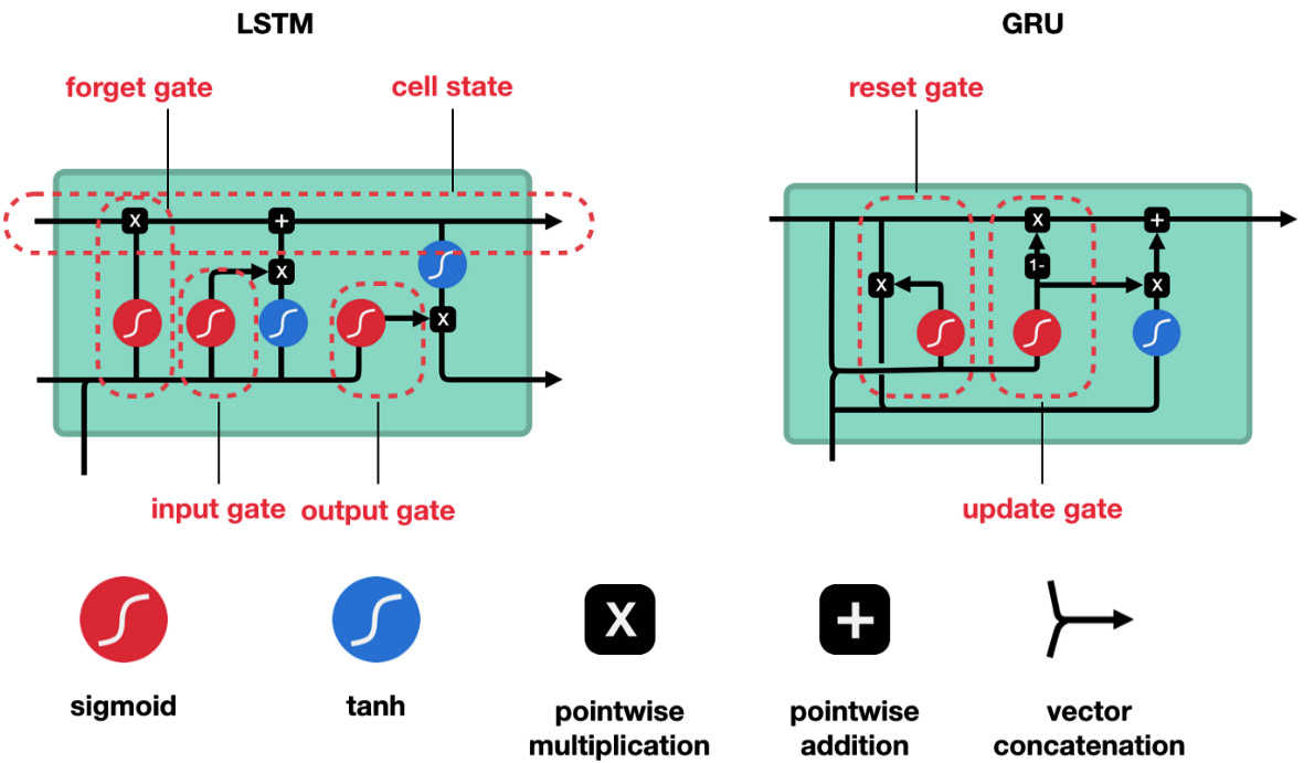
Figure 12.6 – A gating diagram of LSTM versus GRU
The GRU layer in PyTorch
Now, let’s understand the PyTorch implementation of the GRU. The APIs, inputs, and outputs are the same as with an RNN. The API for this can be referenced here: https://pytorch.org/docs/stable/generated/torch.nn.GRU.html#torch.nn.GRU. The key difference is the internal workings of the modules, where the GRU update equations are used instead of the standard RNN ones.
Now, let’s initialize a GRU module and use the synthetic data we have been using to see it in action:
Gru = nn.GRU(
    input_size=1,
    hidden_size=32,
    num_layers=5,
    batch_first=True,
    dropout=0,
    # bidirectional=True,
)
output, hidden_states = gru(rnn_input)
output.shape # -> [6, 15, 32]
hidden_states.shape # -> [5, 6, 32]
Now, let’s look at another major component that can be used for sequential data.
Convolution networks
Convolution networks, also called convolutional neural networks (CNNs), are like neural networks for processing data in the form of a grid. This grid can be 2D, such as an image, 1D, such as a time series, 3D, such as data from LIDAR sensors, and so on. The basic idea behind CNNs is inspired by how human vision works. In 1979, Fukushima proposed Neocognitron. It was a one-of-a-kind architecture that was directly inspired by how human vision works. But CNNs came into existence as we know them today in 1989 when Yann LeCun used backpropagation to learn such a network and proved it by getting state-of-the-art results in handwritten digit recognition. In 2012, when AlexNet (a CNN architecture for image recognition) won the annual challenge of image recognition called ImageNet, that too by a large margin between it and competing non-deep learning approaches, the interest and research in CNNs peaked. People soon figured out that, apart from images, CNNs are effective with sequences, such as language and time series data.
Convolution
At the heart of CNNs is a mathematical operation called convolution. The mathematical interpretation of a convolution operation is beyond the scope of this book, but there are a couple of links in the Further reading section if you want to learn more. For our purposes, we’ll develop an intuitive understanding of the convolution operation. Since CNNs rose to popularity on image data, let’s start by discussing the image domain and then transition to the sequence domain.
Any image (for simplicity, let’s assume it’s grayscale) can be considered as a grid of pixel values, each value denoting how bright that point is, with 1 being pure white and 0 being pure black. Before we start talking about convolution, let’s understand what a kernel is. For now, let’s think of a kernel as a 2D matrix with some values in it. Typically, the kernel’s size is smaller than the image’s size we are using. Since the kernel is smaller than the image, we can “fit” the kernel inside the image. Let’s start with the kernel aligned on the left top edge. With the kernel at the current position, there is a set of values in the image that this kernel is superpositioned over. We can perform element-wise multiplication between this subset of the image and the kernel, and then sum up all the elements into a single scalar. Now, we can repeat this process by “sliding” the kernel into all positions in the image. For instance, the following shows a sample image input whose size is 4x4 and how a convolution operation is carried out on that using a kernel whose size is 2x2:

Figure 12.7 – A convolution operation on 2D and 1D inputs
So, if we place the 2x2 kernel at the top left position and perform the element-wise multiplication and the summation, we get the top left item in the 3x3 output. If we slide the kernel by one position to the right, we get the next element in the top row of the output, and so on. Similarly, if we slide the kernel by one position down, we get the second element in the first column in the output.
While this is interesting, we want to understand convolutions from a time series perspective. To do so, let’s shift our paradigm to 1D convolutions – convolutions performed on 1-dimensional data such as a sequence. In the preceding diagram, we can also see an example of a 1D convolution where we take the 1D kernel and slide it across the sequence to get an output of 1x3.
Although we have set the kernel weights so that they’re convenient to understand and compute, in practice, these weights are learned by the network from data. If we set the kernel size as ![]() and all the kernel weights as
and all the kernel weights as ![]() , what would such a convolution give us? This is something we covered in Chapter 6, Feature Engineering for Time Series Forecasting. Yes, they result in the rolling means with a window of
, what would such a convolution give us? This is something we covered in Chapter 6, Feature Engineering for Time Series Forecasting. Yes, they result in the rolling means with a window of ![]() . Remember, we learned this as a feature engineering technique for machine learning models. So, 1D convolutions can be thought of as a more powerful feature generator, where the features are learned from data. With different weights on the kernels, we will be extracting different features. It is this intuition that we should hold on to while learning CNNs for time series data.
. Remember, we learned this as a feature engineering technique for machine learning models. So, 1D convolutions can be thought of as a more powerful feature generator, where the features are learned from data. With different weights on the kernels, we will be extracting different features. It is this intuition that we should hold on to while learning CNNs for time series data.
Padding, stride, and dilations
Now that we have understood what a convolution operation is, we need to understand a few more terms, such as padding, stride, and dilations.
Before we start talking about these terms, let’s look at an equation that gives the output dimensions (![]() ) of a convolutional layer, given the input dimensions (
) of a convolutional layer, given the input dimensions (![]() ), kernel size (
), kernel size (![]() ), padding size (
), padding size (![]() for left padding and
for left padding and ![]() for right padding), stride (
for right padding), stride (![]() ), and dilation (
), and dilation (![]() ):
):

The default values (padding, strides, and dilations are special cases of a convolution process) of these terms are ![]() . Don’t worry if you don’t understand the formula or the terms in it – just keep the default values in mind so that when we understand each term, we can negate the others.
. Don’t worry if you don’t understand the formula or the terms in it – just keep the default values in mind so that when we understand each term, we can negate the others.
In Figure 12.7, we noticed that the convolution operation always reduces the size of the input. So, in the default case, the formula becomes ![]() . This is because the earliest position we can place the kernel in the sequence is from
. This is because the earliest position we can place the kernel in the sequence is from ![]() to
to ![]() . Then, by convolving through the sequence, we get
. Then, by convolving through the sequence, we get ![]() terms in the output. Padding is when we add some values to the beginning or the end of the sequence. The value we use for padding is dependent on the problem. Typically, we choose zero as a padding value. So, padding a sequence essentially increases the size of the input. So, in the preceding formula, we can think of
terms in the output. Padding is when we add some values to the beginning or the end of the sequence. The value we use for padding is dependent on the problem. Typically, we choose zero as a padding value. So, padding a sequence essentially increases the size of the input. So, in the preceding formula, we can think of ![]() as the effective length of the sequence after padding.
as the effective length of the sequence after padding.
The next two terms (stride and dilation) are closely related to the receptive field of the convolutional layer. The receptive field of a convolutional layer is the region in the input space that influences the feature that’s generated by the convolutional layer. Or, in other words, it is the size of the window of input over which we have performed the convolution operation. For a single convolutional layer (with default settings), this is pretty much the kernel size. For multi-layered CNNs, this calculation becomes a bit more complicated because of the hierarchical structure (the Further reading section contains a link to a paper by Arujo et al. who derived a formula to calculate the receptive field of a CNN). But generally, increasing the receptive field of a CNN is associated with an increase in the accuracy of the CNN. For computer vision, Araujo et al. noted the following:
In time series, this is important because if the receptive field of a CNN is smaller than the long-term dependency, such as the seasonality, that we want to capture, then the network will fail to do so. Making the CNN deeper by stacking more convolutional layers on top of the others is one way to increase the receptive field of a network. But there are a few ways to increase the receptive field of a single convolutional layer. Strides and dilations are two such ways:
- Stride: Earlier, when we talked about sliding the kernel over the sequence, we mentioned that we move the kernel by one position at a time. This is called the stride of the convolutional layer and there is no necessity that the stride should be 1. If we set the stride to 2, the convolution operation would be performed by skipping a position in between, as shown in Figure 12.8. This can make each layer in the convolutional network look at a larger slice of history, thereby increasing the receptive field.
- Dilation: Another way we can tweak the basic convolutional layer is by dilating the input connections. In the standard convolutional layer with a kernel size of 3, we apply the kernel to three consecutive elements in the input with a dilation of 1. If we increase the dilation to 2, then the kernel will be dilated spatially and will be applied. Instead of being applied to three consecutive elements, an element in between will be skipped. Figure 12.8 shows how this works. As we can see, this can also increase the receptive field of the network.
Both these techniques are similar but different and are compatible with each other. The following diagram shows what happens when we apply strides and dilations together (although this doesn’t happen frequently):
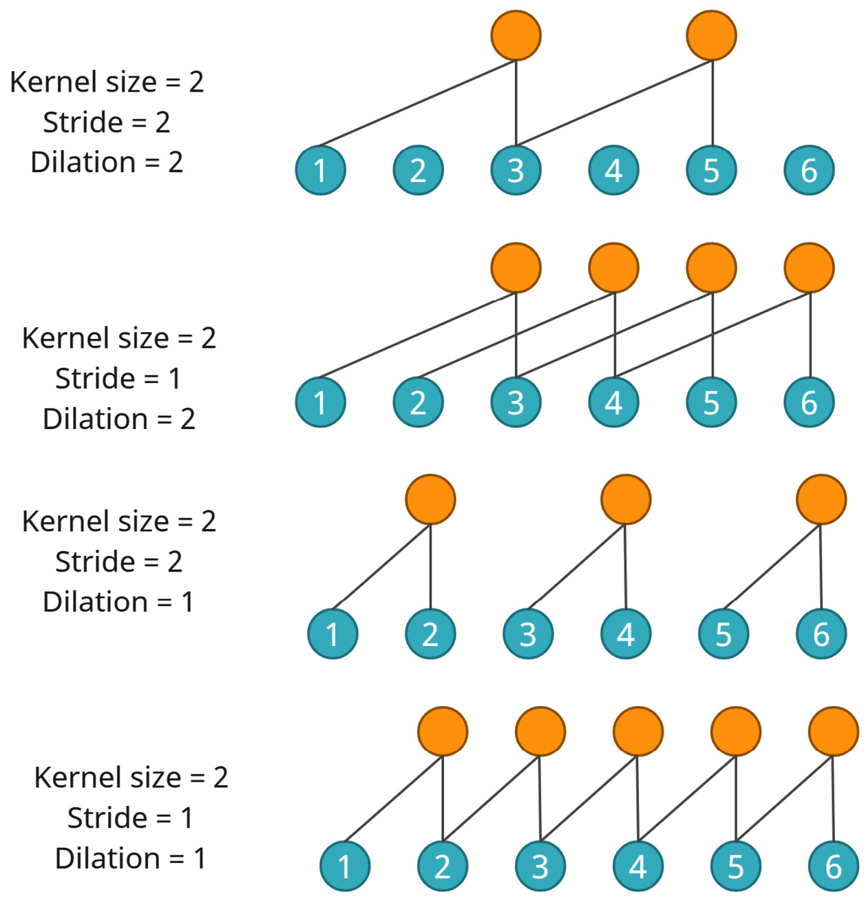
Figure 12.8 – Strides and dilations in convolutions
Now, what if we want to make the output dimensions the same as the input dimensions? By using some basic algebra and rearranging the previous formula, we get the following:

And in time series, we typically pad on the left rather than the right because of the strong autocorrelation that is typically present. Padding the latest few entries with zeros or some other values will make the learning of the prediction function very hard because the latest hidden states are directly influenced by the padded values. The Further reading section contains a link to an article by Kilian Batzner about autoregressive convolutions. It is a must-read if you wish to really understand the concepts we have discussed here and also understand a few limitations. The Further reading section also contains a link to a GitHub repository that contains animations of convolutions for 2D inputs, which will give you a good intuition of what is happening.
There is just one more term that you may hear often in convolutions, especially in time series – causal convolutions. But all you have to keep in mind is that causal convolutions are not special types of convolutions. So long as we ensure that we won’t be using future time steps to predict the current timestep while training, we are performing causal operations. This is typically done by offsetting the target and padding the inputs.
The convolution layer in PyTorch
Now, let’s understand the PyTorch implementation of the CNN (a one-dimensional CNN, which is typically used for sequences such as time series). Let’s look at the different parameters the implementation provides while initializing. We have just discussed the following terms, so they should be familiar to you by now:
- in_channels: The number of expected features in the input. If we are using just the history of the time series, then this would be 1. But when we use history along with some other features, then this will be >1. For subsequent layers, out_channels you have used in the previous layer become your in_channels in the current layer.
- out_channels: The number of kernels or filters applied to the input. Each kernel/filter produces a convolution operation with its own weights.
- kernel_size: This is the size of the kernel we use for convolving.
- stride: The stride of the convolution. The default is 1.
- padding: This is the padding that is added to both sides. If we set the value as 2, the sequence that we pass to the layer will have a padded position on both the left and right. We can also give valid or same as input. These are easy ways of mentioning the kind of padding we need to add. padding=’valid’ is the same as no padding. padding=’same’ pads the input so that the output has the shape as the input. However, this mode doesn’t support any stride values other than 1. The default is 0.
- padding_mode: This defines how the padded positions should be filled with values. The most common and default option is zeros, where all the padded tokens are filled with zeros. Another useful mode that is relevant for time series is replicate, which behaves like forward and backward fill in pandas. The other two options – reflect and circular – are more esoteric and are only used for specific use cases. The default is zeros.
- dilation: The dilation of the convolution. The default is 1.
- groups: This parameter lets you control the way input channels are connected to output channels. The number specified in groups specifies how many groups will be formed so that the convolutions happen within a group and not across. For instance, group=2 means that half the input channels will be convolved by one set of kernels and that the other half will be convolved by a separate set of kernels. This is equivalent to running two convolution layers side by side. Check the documentation for more information on this parameter. Again, this is for an esoteric use case. The default is 1.
- bias: This parameter adds a learnable bias to the convolutions. The default is True.
Let’s apply a CNN model to the same synthetic data we generated earlier in this chapter with a kernel size of 3:
conv = nn.Conv1d(in_channels=1, out_channels=1, kernel_size=k)
Now, let’s look at the inputs and outputs that are expected from a CNN.
Conv1d expects the inputs to have three dimensions – (batch size, number of channels, sequence length). For the initial input layer, the number of channels is the number of features you are feeding into the network; for intermediate layers, it is the number of kernels we have used in the previous layer. The output from Conv1d is in the form of (batch size, number of channels (output), sequence length (output)).
So, let’s run our sequence through Conv1d and look at the inputs and outputs (for more detailed steps, refer to the 02-Building Blocks.ipynb notebook):
#input dim: torch.Size([6, 1, 15])
# batch size = 6, number of features = 1 and sequence length = 15
output = conv(cnn_input)
# Output should be in_dim - k + 1
assert output.size(-1)==cnn_input.size(-1)-k+1
output.shape #-> torch.Size([6, 1, 13])
The notebook provides a slightly more detailed analysis of Conv1d, with tables showing the impact that the hyperparameters have on the shape of the output, what kind of padding is used to make the input and output dimensions the same, and how a convolution with equal weights is just like a rolling mean. I highly suggest that you check it out and play around with the different options to get a feel of what the layer does for you.
Additional information
The inbuilt padding in Conv1d has its roots in image processing, so the padding technique defaults to adding adding to both sides. But for sequences, it is preferable to use padding on the left and because of that, it is also preferable to handle how the input sequences are padded separately and not use the inbuilt mechanism. torch.nn.functional has a handy method called pad that can be used to this effect.
Other building blocks are used in time series forecasting because the architecture of a deep neural network is only limited by creativity. But the point of this chapter was to introduce you to the common ones that appear in many different architectures. We also intentionally left out one of the most popular architectures used nowadays: the transformer. This is because we have devoted another chapter (Chapter 14, Attention and Transformers for Time Series) to understanding attention before we look at transformers. Another major block that is slowly gaining popularity is graph neural networks, which can be thought of as specialized CNNS that operate on graph-based data rather than grids. However, this is outside the scope of this book since it is an area of active research.
Summary
After introducing deep learning in the previous chapter, in this chapter, we gained a deeper understanding of the common architectural blocks that are used for time series forecasting. The encoder-decoder paradigm was explained as a fundamental way we can structure a deep neural network for forecasting. Then, we learned about FFNs, RNNS, and CNNs and explored how they are used to process time series. We also saw how we can use all these major blocks in PyTorch by using the associated notebook and got our hands dirty with some PyTorch code.
In the next chapter, we’ll learn about a few major patterns we can use to arrange these blocks to perform time series forecasting.
References
The following references were used in this chapter:
- Neco, R. P., and Forcada, M. L. (1997), Asynchronous translations with recurrent neural nets. Neural Networks, 1997., International Conference on (Vol. 4, pp. 2535–2540). IEEE: https://ieeexplore.ieee.org/document/614693.
- Kalchbrenner, N., and Blunsom, P. (2013), Recurrent Continuous Translation Models. EMNLP (Vol. 3, No. 39, p. 413): https://aclanthology.org/D13-1176/.
- Kyunghyun Cho, Bart van Merriënboer, Caglar Gulcehre, Dzmitry Bahdanau, Fethi Bougares, Holger Schwenk, and Yoshua Bengio. (2014), Learning Phrase Representations using RNN Encoder-Decoder for Statistical Machine Translation. Proceedings of the 2014 Conference on Empirical Methods in Natural Language Processing (EMNLP), pages 1724–1734, Doha, Qatar. Association for Computational Linguistics: https://aclanthology.org/D14-1179/.
- Ilya Sutskever, Oriol Vinyals, and Quoc V. Le. (2014), Sequence to sequence learning with neural networks. Proceedings of the 27th International Conference on Neural Information Processing Systems – Volume 2: https://dl.acm.org/doi/10.5555/2969033.2969173.
- Rumelhart, D., Hinton, G., and Williams, R (1986). Learning representations by back-propagating errors. Nature 323, 533–536: https://doi.org/10.1038/323533a0.
- Schuster, M., and Paliwal, K. K. (1997). Bidirectional recurrent neural networks. IEEE Transactions on Signal Processing, 45(11), 2673–2681: https://doi.org/10.1109/78.650093.
- Sepp Hochreiter (1991) Untersuchungen zu dynamischen neuronalen Netzen. Diploma thesis, TU Munich: https://people.idsia.ch/~juergen/SeppHochreiter1991ThesisAdvisorSchmidhuber.pdf.
- Y. Bengio, P. Frasconi, and P. Simard (1993), The problem of learning long-term dependencies in recurrent networks. IEEE International Conference on Neural Networks, pp. 1183-1188 vol.3: 10.1109/ICNN.1993.298725.
- Y. Bengio, P. Simard, and P. Frasconi (1994) Learning long-term dependencies with gradient descent is difficult in IEEE Transactions on Neural Networks, vol. 5, no. 2, pp. 157–166, March 1994: 10.1109/72.279181.
- Hochreiter, S., and Schmidhuber, J. (1997). Long short-term memory. Neural computation, 9(8), 1735–1780: https://doi.org/10.1162/neco.1997.9.8.1735.
- Cho, K., Merrienboer, B.V., Gülçehre, Ç., Bahdanau, D., Bougares, F., Schwenk, H., and Bengio, Y. (2014). Learning Phrase Representations using RNN Encoder-Decoder for Statistical Machine Translation. EMNLP: https://www.aclweb.org/anthology/D14-1179.pdf.
- Fukushima, K. Neocognitron: A self-organizing neural network model for a mechanism of pattern recognition unaffected by shift in position. Biol. Cybernetics 36, 193–202 (1980): https://doi.org/10.1007/BF00344251.
- Y. Le Cun, B. Boser, J. S. Denker, R. E. Howard, W. Habbard, L. D. Jackel, and D. Henderson. 1990. Handwritten digit recognition with a back-propagation network. Advances in neural information processing systems 2. Morgan Kaufmann Publishers Inc., San Francisco, CA, USA, 396–404: https://proceedings.neurips.cc/paper/1989/file/53c3bce66e43be4f209556518c2fcb54-Paper.pdf.
Further reading
Take a look at the following resources to learn more about the topics that were covered in this chapter:
- Official PyTorch Tutorials: https://pytorch.org/tutorials/beginner/basics/intro.html
- Essence of linear algebra, by3Blue1Brown: https://www.youtube.com/playlist?list=PLZHQObOWTQDPD3MizzM2xVFitgF8hE_ab
- Neural Networks – A Linear Algebra Perspective, by Manu Joseph: https://deep-and-shallow.com/2022/01/15/neural-networks-a-linear-algebra-perspective/
- Deep Learning, by Ian Goodfellow, Yoshua Bengio,and Aaron Courville: https://deep-and-shallow.com/2022/01/15/neural-networks-a-linear-algebra-perspective/
- Understanding LSTMs, by Christopher Olah: http://colah.github.io/posts/2015-08-Understanding-LSTMs/
- Intuitive Guide to Convolution: https://betterexplained.com/articles/intuitive-convolution/
- Computing Receptive Fields of Convolutional Neural Networks, by Andre Araujo, Wade Norris, and Jack Sim: https://distill.pub/2019/computing-receptive-fields/
- Convolutions in Autoregressive Neural Networks, by Kilian Batzner: https://theblog.github.io/post/convolution-in-autoregressive-neural-networks/
- Convolution Arithmetic, by Vincent Dumoulin and Francesco Visin: https://github.com/vdumoulin/conv_arithmetic
- Dropout: A Simple Way to Prevent Neural Networks from Overfitting, by Nitish Srivastava et al: https://jmlr.org/papers/v15/srivastava14a.html