16

Specialized Deep Learning Architectures for Forecasting

Our journey through the world of deep learning (DL) is coming to an end. In the previous chapter, we were introduced to the global paradigm of forecasting and saw how we can make a simple model such as a Recurrent Neural Network (RNN) perform close to the high benchmark set by global machine learning models. In this chapter, we are going to review a few popular DL architectures that were designed specifically for time series forecasting. With these more sophisticated model architectures, we will be better equipped at handling problems in the wild that call for more powerful models than vanilla RNNs and LSTMs.

In this chapter, we will be covering these main topics:

• The need for specialized architectures
• Neural Basis Expansion Analysis for Interpretable Time Series Forecasting (N-BEATS)
• Neural Basis Expansion Analysis for Interpretable Time Series Forecasting with Exogenous Variables (N-BEATSx)
• Neural Hierarchical Interpolation for Time Series Forecasting (N-HiTS)
• Informer
• Autoformer
• Temporal Fusion Transformer (TFT)
• Interpretability
• Probabilistic forecasting

Technical requirements

You will need to set up an Anaconda environment by following the instructions in the Preface to get a working environment with all the packages and datasets required for the code in this book.

The code associated with this chapter can be found at https://github.com/PacktPublishing/Modern-Time-Series-Forecasting-with-Python/tree/main/notebooks/Chapter16.

You will need to run the following notebooks for this chapter:

• 02-Preprocessing London Smart Meter Dataset.ipynb in Chapter02
• 01-Setting up Experiment Harness.ipynb in Chapter04
• 01-Feature Engineering.ipynb in Chapter06

The need for specialized architectures

Inductive bias, or learning bias, refers to a set of assumptions a learning algorithm makes to generalize the function it learns on training data to unseen data. Deep learning is thought to be a completely data-driven approach where the feature engineering and final task are learned end-to-end, thus avoiding the inductive bias that the modelers bake in while designing the features. But that view is not entirely correct. These inductive biases, which used to be put in through the features, now make their way through the design of architecture. Every DL architecture has its own inductive biases, which is why some types of models perform better on some types of data. For instance, a Convolutional Neural Network (CNN) works well on images, but not as much on sequences because the spatial inductive bias and translational equivariance that the CNN brings to the table are most effective on images.

In an ideal world, we would have an infinite supply of good, annotated data and we would be able to learn entirely data-driven networks with no strong inductive biases. But sadly, in the real world, we will never have enough data to learn such complex functions. This is where designing the right kind of inductive biases makes or breaks the DL system. We used to heavily rely on RNNs for sequences and they had a strong auto-regressive inductive bias baked into them. But later, Transformers, which have a much weaker inductive bias for sequences, came in and with large amounts of data, they were able to learn better functions for sequences. Therefore, this decision about how strong an inductive bias we bake into models is an important question in designing DL architectures.

Over the years, many DL architectures have been proposed specifically for time series forecasting and each of them has its own inductive biases attached to it. We’ll not be able to review every single one of those models, but we will cover the major ones that made a lasting impact on the field. We will also look at how we can use a few open source libraries to train those models on our data. We will exclusively focus on models that can handle the global modeling paradigm, directly or indirectly. This is because of the infeasibility of training separate models for each time series when we are forecasting at scale.

We are going to look at a few popular architectures developed for time series forecasting. One of the major factors influencing the inclusion of a model is also the availability of stable open source frameworks that support these models. This is in no way a complete list because there are many architectures we are not covering here. I’ll try and share a few links in the Further reading section to get you started on your journey of exploration.

Now, without further ado, let’s get started on the first model on the list.

Neural Basis Expansion Analysis for Interpretable Time Series Forecasting (N-BEATS)

The first model that used some components from DL (we can’t call it DL because it is essentially a mix of DL and classical statistics) and made a splash in the field was a model that won the M4 competition (univariate) in 2018. This was a model by Slawek Smyl from Uber (at the time) and was a Frankenstein-style mix of exponential smoothing and an RNN, dubbed ES-RNN (Further reading has links to a newer and faster implementation of the model that uses GPU acceleration). This led to Makridakis et al. putting forward an argument that “hybrid approaches and combinations of methods are the way forward.” The creators of the N-BEATS model aspired to challenge this conclusion by designing a pure DL architecture for time series forecasting. They succeeded in this when they created a model that beat all other methods in the M4 competition (although they didn’t publish it in time to participate in the competition). It is a very unique architecture, taking a lot of inspiration from signal processing. Let’s take a deeper look and understand the architecture.

Reference check

The research paper by Makridakis et al. and the blog post by Slawek Smyl are cited in the References section as 1 and 2, respectively.

We need to establish a bit of context and terminology before moving ahead with the explanation. The core problem that they are solving is univariate forecasting, which means it is similar to classical methods such as exponential smoothing and ARIMA in the sense that it takes only the history of the time series to generate a forecast. There is no provision to include other covariates in the model. The model is shown a window from the history and is asked to predict the next few timesteps. The window of history is referred to as the lookback period and the future timesteps are the forecast period.

The architecture of N-BEATS

The N-BEATS architecture is different from the existing architectures (at the time) in a few aspects:

• Instead of the common encoder-decoder (or sequence-to-sequence) formulation, N-BEATS formulates the problem as a multivariate regression problem.
• Most of the other architectures at the time were relatively shallow (~5 LSTM layers). However, N-BEATS used the residual principle to stack many basic blocks (we will explain this shortly) and the paper has shown that we can stack up to 150 layers and still facilitate efficient learning.
• The model lets us extend it to human interpretable output, still in a principled way.

Let’s look at the architecture and go deeper:

Figure 16.1 – N-BEATS architecture

We can see three columns of rectangular blocks, each one an exploded view of another. Let’s start at the left most (which is the most granular view) and then go up step by step, building up to the architecture. At the top, there is a representative time series, which has a lookback window and a forecast period.

Blocks

The fundamental learning unit in N-BEATS is a block. Each block, , takes in an input, (), of the size of the lookback period and generates two outputs: a forecast, (), and a backcast, (). The backcast is the block’s own best prediction of the lookback period. It is synonymous with fitted values in the classical sense; they tell us how the stack would have predicted the lookback window using the function it has learned. The block input is first processed by a stack of four standard fully connected layers (complete with a bias term and non-linear activation), transforming the input into a hidden representation, . Now, this hidden representation is transformed by two separate linear layers (no bias or non-linear activation) to something the paper calls expansion coefficients for the backcast and forecast, and , respectively. The last part of the block takes these expansion coefficients and maps them to the output using a set of basis layers ( and ). We will talk about the basis layers in a bit more detail later, but for now, just understand that they take the expansion coefficients and transform them into the desired outputs ( and ).

Stacks

Now, let’s move one layer up the abstraction to the middle column of Figure 16.1. It shows how different blocks are arranged in a stack, . All the blocks in a stack share the same kind of basis layers and therefore are grouped as a stack. As we saw earlier, each block has two outputs, and . The blocks are arranged in a residual manner, each block processing and cleaning the time series step by step. The input to a block, , is . At each step, the backcast generated by the block is subtracted from the input to that block before it’s passed on to the next layer. And all the forecast outputs of all the blocks in a stack are added up to make the stack forecast:

The residual backcast from the last block in a stack is the stack residual ().

The overall architecture

With that, we can move to the rightmost column of Figure 16.1, which shows the top-level view of the architecture. We saw that each stack has two outputs – a stack forecast () and stack residual (). There can be N stacks that make up the N-BEATS model. Each stack is chained together so that for any stack (s), the stack residual out of the previous stack () is the input and the stack generates two outputs: the stack forecast () and the stack residual (). Finally, the N-BEATS forecast, , is the additive sum of all the stack forecasts:

Now that we have understood what the model is doing, we need to come back to one point that we left for later – basis functions.

Disclaimer

The explanation here is to mostly aid intuition, so we might be hand-waving over a few mathematical concepts. For a more rigorous treatment of the subject, you should refer to mathematical books/articles that cover the topic. For example, Functions as Vector Spaces from the Further reading section and Function Spaces (https://cns.gatech.edu/~predrag/courses/PHYS-6124-12/StGoChap2.pdf).

Basis functions and interpretability

To understand what basis functions are, we need to understand a concept from linear algebra. We talked about vector spaces in Chapter 11, Introduction to Deep Learning, and gave you a geometric interpretation of vectors and vector spaces. We talked about how a vector is a point in the n-dimensional vector space. We had that discussion regarding regular Euclidean space (), which is intended to represent physical space. Euclidean spaces are defined with an origin and an orthonormal basis. An orthonormal basis is a unit vector (magnitude=1) and they are orthogonal (in simple intuition, at 90 degrees) to each other. Therefore, a vector, , can be written as , where and are the orthonormal basis. You may remember this from high school.

Now, there is a branch of mathematics that views a function as a point in a vector space (at which point we call it a functional space). This comes from the fact that all the mathematical conditions that need to be satisfied for a vector space (things such as additivity, associativity, and so on) are valid if we consider functions instead of points. To better drive that intuition, let’s consider a function, . We can consider this function as a vector in the function space with basis and . Now, the coefficients, 2 and 4, can be changed to give us different functions; this can be any real number from - to +. This space of all functions that can have a basis of and is the functional space, and every function in the function space can be defined as a linear combination of the basis functions. We can have the basis of any arbitrary function, which gives us a lot of flexibility. From a machine learning perspective, searching for the best function in this functional space automatically means that we are restricting the function search so that we have some properties defined by the basis functions.

Coming back to N-BEATS, we talked about the expansion coefficients, and , which are mapped to the output using a set of basis layers ( and ). A basis layer can also be thought of as a basis function because we know that a layer is nothing but a function that maps its inputs to its outputs. Therefore, by learning the expansion coefficients, we are essentially searching for the best function that can represent the output but is constrained by the basis functions we choose.

There are two modes in which N-BEATS operates: generic and interpretable. The N-BEATS paper shows that under both modes, N-BEATS managed to beat the best in the M4 competition. Generic mode is where we do not have any basis function constraining the function search. We can also think of this as setting the basis function to be the identity function. So, in this mode, we are leaving the function completely learned by the model through a linear projection of the basis coefficients. This mode lacks human interpretability because we don’t have any idea how the different functions are learned and what each stack signifies.

But if we have fixed basis functions that constrain the function space, we can bring in more interpretability. For instance, if we have a basis function that constrains the output to represent the trends for all the blocks in a stack, we can say that the forecast output of that stack represents the trend component. Similarly, if we have another basis function that constrains the output to represent the seasonality for all the blocks in a stack, we can say that the forecast output of the stack represents seasonality.

This is exactly what the paper has proposed as well. They have defined specific basis functions that capture trend and seasonality, and including such blocks makes the final forecast more interpretable by giving us a decomposition. The trend basis function is a polynomial of a small degree, p. So, as long as p is low, such as 1, 2, or 3, it forces the forecast output to mimic the trend component. And for the seasonality basis function, the authors chose a Fourier basis (similar to the one we saw in Chapter 6, Feature Engineering for Time Series Forecasting). This forces the forecast output to be functions of these sinusoidal basis functions that mimic seasonality. In other words, the model learns to combine these sinusoidal waves with different coefficients to reconstruct the seasonality pattern as best as possible.

For a deeper understanding of these basis functions and how they are structured, I have linked to a Kaggle notebook in the Further reading section that provides a clear explanation of the trend and seasonality basis functions. The associated notebook also has an additional section that visualizes the first few basis functions of seasonality. Along with the original paper, these additional readings will help you solidify your understanding.

N-BEATS wasn’t designed to be a global model, but it does well in the global setting. The M4 competition was a collection of unrelated time series and the N-BEATS model was trained so that the model was exposed to all those series and learned a common function to forecast each time series in the dataset. This, along with ensembling multiple N-BEATS models with different lookback windows, was the success formula for the M4 competition.

Reference check

The research paper by Boris Oreshkin et al (N-BEATS) is cited in the References section as 3.

Forecasting with N-BEATS

N-BEATS is implemented in PyTorch Forecasting. We can use the same framework we worked with in Chapter 15, Strategies for Global Deep Learning Forecasting Models, and extend it to train N-BEATS on our data. First, let’s look at the initialization parameters of the implementation.

The Nbeats class in PyTorch Forecasting has the following parameters:

• stack_types: This defines the number of stacks that we need to have in the N-BEATS model. This should be a list of strings (generic, trend, or seasonality) denoting the number and type of stacks. Examples include ["trend", "seasonality"], ["trend", "seasonality", "generic"], ["generic", "generic", "generic"], and so on. However, if the entire network is generic, we can just have a single generic stack with more blocks as well.
• num_blocks: This is a list of integers signifying the number of blocks in each stack that we have defined. If we had defined stack_types as ["trend", "seasonality"], and we want three blocks each, we can set num_blocks to [3,3].
• num_block_layers: This is a list of integers signifying the number of FC layers with ReLU activation in each block. The recommended value is 4 and the length of the list should be equal to the number of stacks we have defined.
• width: This sets the width or the number of units in the FC layers in each block. This is also a list of integers with lengths equal to the number of stacks defined.
• sharing: This is a list of Booleans signifying whether the weights generating the expansion coefficients are shared with other blocks in a stack. It is recommended to share the weights in the interpretable stacks and not share them in the generic stacks.
• expansion_coefficient_length: This represents the size of the expansion coefficients (). Depending on the kind of block, the intuitive meaning of this parameter changes. For the trend block, this means the number of polynomials we are using in our basis functions. And for the seasonality, this lets us control how quickly the underlying Fourier basis functions vary. The Fourier basis functions are sinusoidal basis functions with different frequencies; if they have a large expansion_coefficient_length, this means that subsequent basis functions will have a larger frequency than if you had a smaller expansion_coefficient_length. This is a parameter that we can tune as a hyperparameter. A typical range can be between 2 and 10.

There are a few other parameters, but these are not as important. A full list of parameters and their descriptions can be found at https://pytorch-forecasting.readthedocs.io/en/stable/api/pytorch_forecasting.models.nbeats.NBeats.html.

Since the strength of the model is in forecasting slightly longer durations, we move from one-step ahead to one-day ahead (48 steps) forecasting. The only change we have to implement is changing the max_prediction_length parameter to 48 instead of 1 while initializing TimeSeriesDataset.

Notebook alert

The complete code for training N-BEATS can be found in the 01-N-BEATS.ipynb notebook in the Chapter16 folder. There are two variables in the notebook that act as switches: TRAIN_SUBSAMPLE = True makes the notebook run for a subset of 10 households, while train_model = True makes the notebook train different models (warning: training the model on full data takes hours). train_model = False loads the trained model weights (not included in the repository but saved every time you run training) and predicts on them.

Interpreting N-BEATS forecasting

N-BEATS, if we are running it in the interpretable model, also gives us more interpretability by separating the forecast into trend and seasonality. To get the interpretable output, we only need to make a small change in the predict function – we must change mode="prediction" to mode="raw" in the parameters:

best_model.predict(val_dataloader, mode="raw")

This will return us a namedtuple from which trend can be accessed using the trend key, seasonality from the seasonality key, and total predictions from the prediction key. Let’s see how one of the household predictions decomposed:

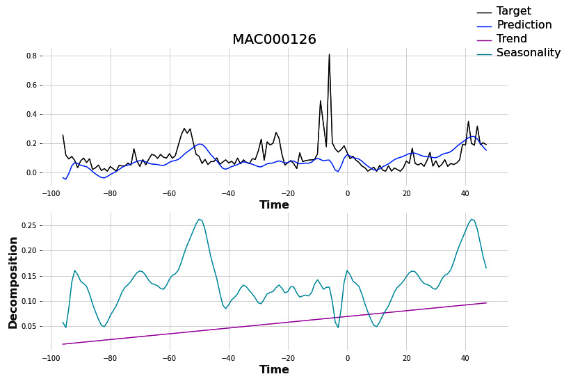
Figure 16.2 – Decomposed predictions from N-BEATS (interpretable)

With all its success, N-BEATS was still a univariate model. It was not able to take in any external information, apart from its history. This was fine for the M4 competition, where all the time series in question were also univariate. But many real-world time series problems come with additional explanatory variables (or exogenous variables). Let’s look at a slight modification that was made to N-BEATS that enabled exogenous variables.

Neural Basis Expansion Analysis for Interpretable Time Series Forecasting with Exogenous Variables (N-BEATSx)

Olivares et al. proposed an extension of the N-BEATS model by making it compatible with exogenous variables. The overall structure is the same (with blocks, stacks, and residual connections) as N-BEATS (Figure 16.1), so we will only be focusing on the key differences and additions that the N-BEATSx model puts forward.

Reference check

The research paper by Olivares et al. (N-BEATSx) is cited in the References section as 4.

Handling exogenous variables

In N-BEATS, the input to a block was the lookback window, . But here, the input to a block is both the lookback window, , and the array of exogenous variables, . These exogenous variables can be of two types: time-varying and static. The static variables are encoded using a static feature encoder. This is nothing but a single-layer FC that encodes the static information into a dimension specified by the user. Now, the encoded static information, the time-varying exogenous variables, and the lookback window are concatenated to form the input for a block so that the hidden state representation, , of block is not like in N-BEATS, but , where represents concatenation. This way, the exogenous information is part of the input to every block as it is concatenated with the residual at each step.

Exogenous blocks

In addition to this, the paper also proposes a new kind of block – an exogenous block. The exogenous block takes in the concatenated lookback window and exogenous variables (just like any other block) as input and produces a backcast and forecast:

Here, is the number of exogenous features.

Here, we can see that the exogenous forecast is the linear combination of the exogenous variables and that the weights for this linear combination are learned by the expansion coefficients, . The paper refers to this configuration as the interpretable exogenous block because by using the expansion weights, we can define the importance of each exogenous variable and even figure out the exact part of the forecast, which is because of a particular exogenous variable.

N-BEATSx also has a generic version (which is not interpretable) of the exogenous block. In this block, the exogenous variables are passed through an encoder that learns a context vector, , and the forecast is generated using the following formula:

They proposed two encoders: a Temporal Convolutional Network (TCN) and WaveNet (a network similar to the TCN, but with dilation to expand the receptive field). The Further reading section contains resources if you wish to learn more about WaveNet, an architecture that originated in the sound domain.

Additional information

N-BEATSx is not implemented in PyTorch Forecasting, but we can find it in another library for forecasting using DL – neuralforecast by Nixtla. One feature that neuralforecast lacks (which is kind of a deal breaker to me) is that it doesn’t support categorical features. So, we will have to encode the categorical features into numerical representations (like we did in Chapter 10, Global Forecasting Models) before using neuralforecast. Also, the documentation of the library isn’t great, which means we need to dive into the code base and hack it to make it work.

The research paper also showed that N-BEATSx outperformed N-BEATS, ES-RNN, and other benchmarks on electricity price forecasting considerably.

Continuing with the legacy of N-BEATS, we will now talk about another modification to the architecture that makes it suitable for long-term forecasting.

Neural Hierarchical Interpolation for Time Series Forecasting (N-HiTS)

Although there has been a good amount of work from DL to tackle time series forecasting, very little focus has been on long-horizon forecasting. Despite recent progress, long-horizon forecasting remains a challenge because of two reasons:

• The expressiveness required to truly capture the variation
• The computational complexity

Attention-based methods (Transformers) and N-BEATS-like methods scale quadratically in memory and the computational cost concerning the forecasting horizon.

The authors claim that N-HiTS drastically cuts long-forecasting compute costs while simultaneously showing 25% accuracy improvements compared to existing Transformer-based architectures across a large array of multi-variate forecasting datasets.

Reference check

The research paper by Challu et al. on N-HiTS is cited in the References section as 5.

The Architecture of N-HiTS

N-HiTS can be considered as an alteration to N-BEATS because the two share a large part of their architectures. Figure 16.1, which shows the N-BEATS architecture, is still valid for N-HiTS. N-HiTS also has stacks of blocks arranged in a residual manner; it differs only in the kind of blocks it uses. For instance, there is no provision for interpretable blocks. All the blocks in N-HiTS are generic. While N-BEATS tries to decompose the signal into different patterns (trend, seasonality, and so on), N-HiTS tries to decompose the signal into multiple frequencies and forecast them separately. To enable this, a few key improvements have been proposed:

• Multi-rate data sampling
• Hierarchical interpolation
• Synchronizing the rate of input sampling with a scale of output interpolation across the blocks

Multi-rate data sampling

N-HiTS incorporates sub-sampling layers before the fully connected blocks so that the resolution of the input to each block is different. This is similar to smoothing the signal with different resolutions so that each block is looking at a pattern that occurs at different resolutions – for instance, if one block looks at the input every day, another block looks at the output every week, and so on. This way, when arranged with different blocks looking at different resolutions, the model will be able to predict patterns that occur in those resolutions. This significantly reduces the memory footprint and the computation required as well, because instead of looking at all H steps of the lookback window, we are looking at smaller series (such as H/2, H/4, and so on).

N-HiTS accomplishes this using a Max Pooling or Average Pooling layer of kernel size on the lookback window. A pooling operation is similar to a convolution operation, but the function that is used is non-learnable. In Chapter 12, Building Blocks of Deep Learning for Time Series, we learned about convolutions, kernels, stride, and so on. While a convolution uses weights that are learned from data while training, a pooling operation uses a non-learnable and fixed function to aggregate the data in the receptive field of a kernel. Common examples of these functions are the maximum, average, sum, and so on. N-HiTS uses MaxPool1d or AvgPool1d (in PyTorch terminology) with different kernel sizes for different blocks. Each pooling operation also has a stride equal to the kernel, resulting in non-overlapping windows over which we do the aggregation operation. To refresh our memory, let’s see what max pooling with kernel=2 and stride=2 looks like:

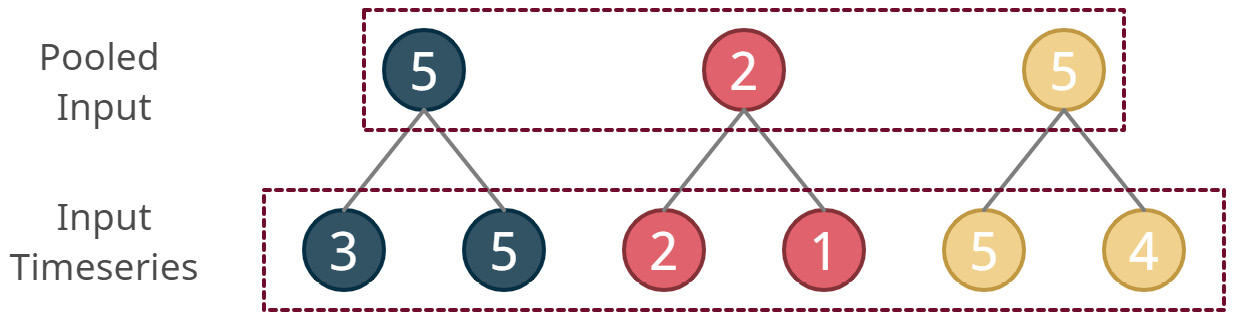
Figure 16.3 – Max pooling on one dimension – kernel=2, stride=2

Therefore, a larger kernel size will tend to cut more high-frequency (or small-timescale) components from the input. This way, the block is forced to focus on larger-scale patterns. The paper calls this multi-rate signal sampling.

Hierarchical interpolation

In a standard multi-step forecasting setting, the model must forecast H timesteps. And as H becomes larger, the compute requirements increase and lead to an explosion of expressive power the model needs to have. Training a model with such a large expressive power, without overfitting, is a challenge in itself. To combat these issues, N-HiTS proposes a technique called temporal interpolation.

The pooled input (which we saw in the previous section) goes into the block along with the usual mechanism to generate expansion coefficients and finally gets converted into forecast output. But here, instead of setting the dimension of the expansion coefficients as H, N-HiTS sets them as , where is the expressiveness ratio. This parameter essentially reduces the forecast output dimension and thus controls the issues we discussed in the previous paragraph. To recover the original sampling rate and predict all the H points in the forecast horizon, we can use an interpolation function. There are many options for the interpolation functions – linear, nearest neighbor, cubic, and so on. All these options can easily be implemented in PyTorch using the interpolate function.

Synchronizing the input sampling and output interpolation

In addition to proposing the input sampling through pooling and output interpolation, N-HiTS also proposes to arrange them in different blocks in a particular way. The authors argue that hierarchical interpolation can only happen the right way if the expressiveness ratios are distributed across blocks in a manner that is synchronized with the multi-rate sampling. Blocks closer to the input should have a smaller expressiveness ratio, , and larger kernel sizes, . This means that the blocks closer to the input will generate larger resolution patterns (because of aggressive interpolation) while being forced to look at aggressively subsampled input signals. The paper proposes exponentially increasing expressiveness ratios as we move from the initial block to the last block to handle a wide range of frequency bands. The official N-HiTS implementation uses the following formula to set the expressiveness ratios and pooling kernels:

pooling_sizes = np.exp2(
    np.round(np.linspace(0.49, np.log2(prediction_length / 2), n_stacks))
)
pooling_sizes = [int(x) for x in pooling_sizes[::-1]]
downsample_frequencies = [
    min(prediction_length, int(np.power(x, 1.5))) for x in pooling_sizes
]

We can also provide explicit pooling_sizes and downsampling_fequencies to reflect known cycles of the time series (weekly seasonality, monthly seasonality, and so on). The core principle of N-BEATS (one block removing the effect it captures from the signal and passing it on to the next block) is used here as well so that, at each level, the patterns or frequencies that a block captures are removed from the input signal before being passed on to the next block. In the end, the final forecast is the sum of all such individual block forecasts.

Forecasting with N-HiTS

N-HiTS is implemented in PyTorch Forecasting. We can use the same framework we were working with in Chapter 15, Strategies for Global Deep Learning Forecasting Models, and extend it to train N-HiTS on our data. What’s even better is that the implementation supports exogenous variables, the same way N-BEATSx handles exogenous variables (although without the exogenous block). First, let’s look at the initialization parameters of the implementation.

The NHiTS class in PyTorch Forecasting has the following parameters:

• n_blocks: This is a list of integers signifying the number of blocks to be used in each stack. For instance, [1,1,1] means there will be three stacks with one block each.
• n_layers: This is either a list of integers or a single integer signifying the number of FC layers with a ReLU activation in each block. The recommended value is 2.
• hidden_size: This sets the width or the number of units in the FC layers in each block.
• static_hidden_size: The static features are encoded using an FC encoder into a dimension that is set by this parameter. We covered this in detail in the Neural Basis Expansion Analysis for Interpretable Time Series Forecasting with Exogenous Variables (N-BEATSx) section.
• shared_weights: This signifies whether the weights generating the expansion coefficients are shared with other blocks in a stack. It is recommended to share the weights in the interpretable stacks and not share them in the generic stacks.
• pooling_sizes: This is a list of integers that defines the pooling size () for each stack. This is an optional parameter, and if provided, we can have more control over how the pooling happens in the different stacks. Using an ordering of higher to lower improves results.
• pooling_mode: This defines the kind of pooling to be used. It should be either 'max' or 'average'.
• downsample_frequencies: This is a list of integers that defines the expressiveness ratios () for each stack. This is an optional parameter, and if provided, we can have more control over how the interpolation happens in the different stacks.

Notebook alert

The complete code for training N-HiTS can be found in the 02-N-HiTS.ipynb notebook in the Chapter16 folder. There are two variables in the notebook that act as switches – TRAIN_SUBSAMPLE = True makes the notebook run for a subset of 10 households, while train_model = True makes the notebook train different models (warning: training the model on full data takes hours). train_model = False loads the trained model weights (not included in the repository but saved every time you run training) and predicts on them.

Now, let’s shift our focus and look at a few modifications of the Transformer model to make it better for time series forecasting.

Informer

Recently, Transformer models have shown superior performance in capturing long-term patterns than standard RNNs. One of the major factors of that is the fact that self-attention, which powers Transformers, can reduce the length that the relevant sequence information has to be held on to before it can be used for prediction. In other words, in an RNN, if the timestep 12 steps before holds important information, that information has to be stored in the RNN through 12 updates before it can be used for prediction. But with self-attention in Transformers, the model is free to create a shortcut between lag 12 and the current step directly because of the lack of recurrence in the structure.

But the same self-attention is also the reason why we can’t scale vanilla Transformers to long sequences. In the previous section, we discussed how long-term forecasting is a challenge because of two reasons: the expressiveness required to truly capture the variation and computational complexity. Self-attention, with its quadratic computational complexity, contributes to the second reason. Scaling Transformers on very long sequences will require us to pour computation into the model using multi-GPU setups, which makes real-world deployment a challenge, especially when good alternative models such as ARIMA, LightGBM, and N-BEATS exist.

The research community has recognized this challenge and has put a lot of effort into devising efficient transformers through many techniques such as downsampling, low-rank approximations, sparse attention, and so on. For a detailed account of such techniques, refer to the link for Efficient Transformers: A Survey in the Further reading section.

Reference check

The research paper by Zhou et al. on the Informer model is cited in the References section as 8.

The architecture of the Informer model

The Informer model is a modification of Transformers. The following are its major contributions:

• Uniform Input Representation: A methodical way to include the history of the series along with other information, which will help in capturing long-term signals such as the week, month, holidays, and so on
• ProbSparse: An efficient attention mechanism based on information theory
• Attention distillation: A mechanism to provide dominating attention scores while stacking multiple layers and also reduce computational complexity
• Generative-style decoder: Used to generate the long-term horizon in a single forward pass instead of via dynamic recurrence

Let’s take a look at the overall architecture (Figure 16.4) to see how they fit together, and then look at them in more detail:

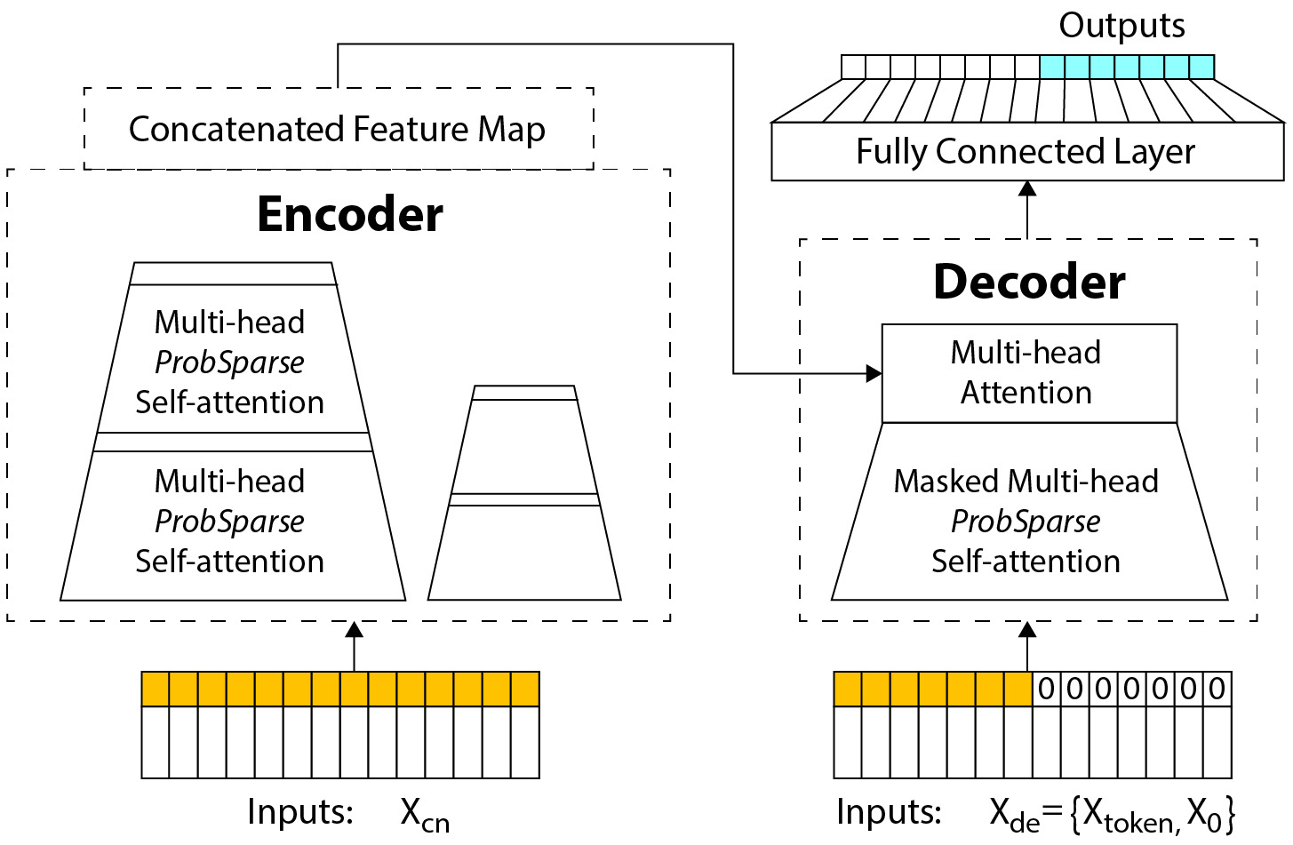
Figure 16.4 – Informer model architecture

The overall architecture is akin to a standard encoder-decoder transformer model. The encoder takes in the inputs and uses multi-headed attention to generate features that are passed to the decoder, which, in turn, uses these features to generate the forecast. Special modifications are made to the architecture in each of these steps. Let’s review them in detail.

Uniform Input Representation

RNNs capture time series patterns with their recurrent structure, so they only need the sequence; they don’t need information about the timestamp to extract the patterns. However, the self-attention in Transformers is done via point-wise operations that are performed in sets (the order doesn’t matter in a set). Typically, we include positional encodings to capture the order of the sequence. Instead of using positional encodings, we can use richer information, such as hierarchical timestamp information (such as weeks, months, years, and so on). This is what the authors proposed through Uniform Input Representation.

Uniform Input Representation uses three types of embeddings to capture the history of the time series, the sequence of values in the time series, and the global timestamp information. The sequence of values in the time series is captured by the standard positional embedding of the d_model dimension.

Uniform Input Representation uses a one-dimensional convolutional layer with kernel=3 and stride=1 to project the history (which is scalar or one-dimensional) into an embedding of d_model dimensions. This is referred to as value embedding.

The global timestamp information is embedded by a learnable embedding of d_model dimensions with limited vocabulary in a mechanism that is identical to embedding categorical variables into fixed-size vectors (Chapter 15, Strategies for Global Deep Learning Forecasting Models). This is referred to as temporal embedding.

Now that we have three embeddings of the same dimension, d_model, all we need to do is add them together to get the Uniform Input Representation.

ProbSparse attention

In Chapter 14, Attention and Transformers for Time Series, we defined a generalized attention model as follows:

Here, is an alignment function that calculates a similarity or a notion of similarity between the queries and keys, is a distribution function that converts this score into attention weights that sum up to 1, and q, k, and v are the query, key, and values of the attention mechanism, respectively.

Additional information

The original Transformer uses scaled dot product attention, along with different projection matrices for the query, key, and values. The formula can be written like so:

Here, , , and are learnable projection matrices for the query, key, and values, respectively, and is the attention dimension. We know that is defined as follows:

Let’s denote as and as . So, using the softmax expansion, we can write the previous formula like so:

Here, denotes the inner product. In 2019, Tsai et al. proposed an alternate view of the attention mechanism using kernels. The math and history behind kernels are quite extensive and are outside the scope of this book. Just know that a kernel is a special kind of function, similar to a similarity function. In this case, if we define as (which is an asymmetric exponential kernel), the attention equation becomes like this:

This interpretation leads to a probabilistic view of attention where the first term is:

Which can be interpreted as the probability of , given , .

The attention equation can also be written as follows:

Here, is the expectation of the probability of , given . The quadratic computational complexity stems from the calculation of this expectation. We will have to use all the elements in the query and the key to calculate a matrix of probabilities.

Previous studies had revealed that this distribution of self-attention probability has potential sparsity. The authors of the paper also reaffirmed this through their experiments. The essence of this sparsity is that there are only a few query-key pairs that absorb the majority of the probability mass. In other words, there will be a few query-key pairs that will have a high probability; the others will be closer to zero. But the key question is to identify which query-key pairs contribute to major attention without doing the actual calculation.

From the re-written attention equation, the -th query’s attention on all the keys is defined as a probability and the output is its composition with values, . If is close to a uniform distribution, will be . This means that self-attention becomes a simple sum of all values. The dominant dot-product query-key pairs encourage the corresponding query’s probability distribution to deviate away from the uniform distribution. So, we can measure how different the attention distribution is from the uniform distribution to measure how dominant a query-key pair is. We can use Kullback-Liebler (KL) Divergence to measure this difference. KL Divergence is based on information theory and is defined as the information loss that happens when one distribution is approximated using the other. Therefore, the more different the two distributions are, the larger the loss, and thereby KL Divergence. In this manner, it measures how much one distribution diverges from another.

The formula for calculating KL Divergence with the uniform distribution works out to be as follows:

The first term here is the Log-Sum-Exp (LSE) of q_i, on all the keys. LSE is known to have numerical stability issues, so the authors proposed an empirical approximation. The complete proof is in the paper for those who are interested. So, after the approximation, the measure of divergence, , becomes as follows:

This still doesn’t absolve us of the quadratic calculation of the dot product of all query-key pairs. But the authors further prove that to approximate this measure of divergence, we only need to randomly sample query-key pairs, where is the length of the query and is the length of the keys. We only calculate the dot product on these sampled pairs and fill zero for the rest of it. Furthermore, we select a sparse Top-u from the calculated probabilities as . It is on this , for which we already have the dot products, we calculate the attention distribution. This considerably reduces the computational load on the self-attention calculation.

Attention distillation

One of the consequences of using ProbSparse attention is that we end up with redundant combinations of values. This is mainly because we might keep sampling the same dominant query-key pairs. The authors propose using a distilling operation to privilege the superior ones with dominating features and make the self-attention feature maps more focused layer after layer. They do this by using a mechanism similar to dilated convolutions. The attention output from each layer is passed through a Conv1d filter with kernel = 3 on the time dimension, an activation (the paper suggests ELU), and a MaxPool1d with kernel = 3 and stride = 2. More formally, the output of a layer j+1 is as follows:

Here, represents the attention block.

Generative-style decoder

The standard way of inferencing a Transformer model is by decoding one token at a time. This autoregressive process is time-consuming and repeats a lot of calculations for each step. To alleviate this problem, the Informer model adopts a more generative fashion where the entire forecasting horizon is generated in a single forward pass.

In NLP, it is a popular technique to use a special token (START) to start the dynamic decoding process. Instead of choosing a special token for this purpose, the Informer model chooses a sample from the input sequence, such as an earlier slice before the output window. For instance, if we say the input window is to , we will sample a sequence of length from the input, to , and include this sequence as the starting sequence of the decoder. And to make the model predict the entire horizon in a single forward pass, we can extend the decoder input tensor so that its length is , where is the length of the prediction horizon. The initial C tokens are filled with the sample sequence from the input, and the rest is filled as zeros – that is, . This is just the target. Although has zeros filled in for the prediction horizon, this is just for the target. The other information, such as the global timestamps, is included in . Sufficient masking of the attention matrix is also employed so that each position does not attend to future positions, thus maintaining the autoregressive nature of the prediction.

Forecasting with the Informer model

Unfortunately, the Informer model has not been implemented in PyTorch Forecasting. However, we have adapted the original implementation by the authors of the paper so that it can work with PyTorch Forecasting; it can be found in src/dl/ptf_models.py in a class named InformerModel. We can use the same framework we worked with in Chapter 15, Strategies for Global Deep Learning Forecasting Models, with this implementation.

Important note

We have to keep in mind that the Informer model does not support exogenous variables. The only additional information it officially supports is global timestamp information such as the week, month, and so on, along with holiday information. We can technically extend this to use any categorical feature (static or dynamic), but no real-valued information is currently supported.

Let’s look at the initialization parameters of the implementation.

The InformerModel class has the following major parameters:

• label_len: This is an integer representing the number of timesteps from the input sequence to sample as a START token while decoding.
• distil: This is a Boolean flag for turning the attention distillation off and on.
• e_layers: This is an integer representing the number of encoder layers.
• d_layers: This is an integer representing the number of decoder layers.
• n_heads: This is an integer representing the number of attention heads.
• d_ff: This is an integer representing the number of kernels in the one-dimensional convolutional layers used in the encoder and decoder layers.
• activation: This is a string that takes in one of two values – relu or gelu. This is the activation to be used in the encoder and decoder layers.
• factor: This is a float value that controls the sparsity of the attention calculation. For a value less than 1, it reduces the number of query-value pairs to calculate the divergence measure and reduces the number of Top-u samples taken than the standard formula for these quantities.
• dropout: This is a float between 0 and 1, which determines the strength of the dropout in the network.

Notebook alert

The complete code for training the Informer model can be found in the 03-Informer.ipynb notebook in the Chapter16 folder. There are two variables in the notebook that act as switches – TRAIN_SUBSAMPLE = True makes the notebook run for a subset of 10 households, while train_model = True makes the notebook train different models (warning: training the model on the full data takes hours). train_model = False loads the trained model weights (not included in the repository but saved every time you run training) and predicts on them.

Now, let’s look at another modification of the Transformer architecture that uses autocorrelation and time series decomposition more effectively.

Autoformer

Autoformer is another model that is designed for long-term forecasting. While the Informer model focuses on making the attention computation more efficient, Autoformer invents a new kind of attention and couples it with aspects from time series decomposition.

The architecture of the Autoformer model

Autoformer has a lot of similarities with the Informer model, so much so that it can be thought of as an extension of the Informer model. Uniform Input Representation and the generative-style decoder have been reused in Autoformer. But instead of ProbSparse attention, Autoformer has an AutoCorrelation mechanism. And instead of attention distillation, Autoformer has a time series decomposition-inspired encoder-decoder setup.

Reference check

The research paper by Wu et al. on Autoformer is cited in the References section as 9.

Let’s look at the time series decomposition architecture first.

Decomposition architecture

We saw this idea of decomposition back in Chapter 3, Analyzing and Visualizing Time Series Data, and even in this chapter (N-BEATS). Autoformer successfully renovated the Transformer architecture into a deep-decomposition architecture:

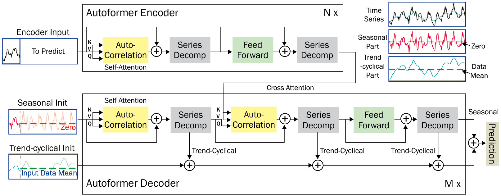
Figure 16.5 – Autoformer architecture

It is easier to understand the overall architecture first and then dive deeper into the details. In Figure 16.5, there are boxes labeled Auto-Correlation and Series Decomp. For now, just know that auto-correlation is a type of attention and that series decomposition is a particular block that decomposes the signal into trend-cyclical and seasonal components.

Encoder

With the level of abstraction discussed in the preceding section, let’s understand what is happening in the encoder:

1. The uniform representation of the time series, , is the input to the encoder. The input is passed through an Auto-Correlation block (for self-attention) whose output is .
2. The uniform representation, , is added back to as a residual connection, ..
3. Now, is passed through a Series Decomp block, which decomposes the signal into a trend-cyclical component () and a seasonal component, .
4. We discard and pass to a Feed Forward network, which gives as an output.
5. is again added to as a residual connection, .
6. Finally, this is passed through another Series Decomp layer, which again decomposes the signal into the trend, , and a seasonal component, .
7. We discard , and pass on as the final output from one block of the encoder.
8. There may be N blocks of encoders stacked together, one taking in the output of the previous encoder as input.

Now, let’s shift our attention to the decoder block.

Decoder

Like the Informer model, the Autoformer model uses a START token-like mechanism by including a sampled window from the input sequence. But instead of just taking the sequence, Autoformer does a bit of special processing on it. Autoformer uses the bulk of its learning power to learn seasonality. The output of the transformer is also just the seasonality. Therefore, instead of including the complete window from the input sequence, Autoformer decomposes the signal and only includes the seasonal component in the START token. Let’s look at this process step by step:

1. If the input (the context window) is , we decompose it with the Series Decomp block into and .
2. Now, we sample timesteps from the end of and append zeros, where is the forecast horizon, and construct .
3. This is then used to create a uniform representation, .
4. Meanwhile, we sample timesteps from the end of and append timesteps with the series mean (), where is the forecast horizon, and construct .

This is then used as the input for the decoder. This is what happens in the decoder:

1. The input, , is first passed through an Auto-Correlation (for self-attention) block whose output is .
2. The uniform representation, , is added back to as a residual connection, ..
3. Now, is passed through a Series Decomp block that decomposes the signal into a trend-cyclical component () and a seasonal component, .
4. In the decoder, we do not discard the trend component; instead, we save it. This is because we will be adding all the trend components with the trend in it () to come up with the overall trend part ().
5. The seasonal output from the Series Decomp block (, along with the output from the encoder (), is then passed into another Auto-Correlation block where cross-attention between the decoder sequence and encoder sequence is calculated. Let the output of this block be .
6. Now, is added back to as a residual connection, .
7. is again passed through a Series Decomp block, which splits into two components – and .
8. is then transformed using a Feed Forward network into and is added to it in a residual connection, .
9. Finally, is passed through yet another Series Decomp block, which decomposes it into two components – and . is the final output of the decoder, which captures seasonality.
10. Another output is the residual trend, , which is a projection of the summation of all the trend components extracted in the decoder’s Series Decomp blocks. The projection layer is a Conv1d layer, which projects the extracted trend to the desired output dimension:

11. such decoder layers are stacked on top of each other, each one feeding its output as the input to the next one.
12. The residual trend, , of each decoder layer gets added to the trend init, , to model the overall trend component ().
13. The of the final decoder layer is considered to be the overall seasonality component and is projected to the desired output dimension () using a linear layer.
14. Finally, the prediction or the forecast .

The whole architecture is cleverly designed so that the relatively stable and easy-to-predict part of the time series (the trend-cyclical) is removed and the difficult-to-capture seasonality can be modeled well.

Now, how does the Series Decomp block decompose the series? The mechanism may be familiar to you already: AvgPool1d with some padding so that it maintains the same size as the input. This acts like a moving average over the specified kernel width.

We have been talking about the Auto-Correlation block throughout this explanation. Now, let’s understand the ingenuity of the Auto-Correlation block.

Auto-correlation mechanism

Autoformer uses an auto-correlation mechanism in place of standard scaled dot product attention. This discovers sub-series similarity based on periodicity and uses this similarity to aggregate similar sub-series. This clever mechanism breaks the information bottleneck by expanding the point-wise operation of the scaled dot product attention to a sub-series level operation. The initial part of the overall mechanism is similar to the standard attention procedure, where we project the query, key, and values into the same dimension using weight matrices. The key difference is the attention weight calculation and how they are used to calculate the values. This mechanism achieves this by using two salient sub-mechanisms: discovering period-based dependencies and time delay aggregation.

Period-based dependencies

Autoformer uses autocorrelation as the key measure of similarity. Auto-correlation, as we know, represents the similarity between a given time series, , and its lagged series. For instance, is the autocorrelation between the time series and . Autoformer considers this autocorrelation as the unnormalized confidence of the particular lag. Therefore, from the list of all , we choose most possible lags and use softmax to convert these unnormalized confidences into probabilities. We use these probabilities as weights to aggregate relevant sub-series (we will talk about this in the next section).

The autocorrelation calculation is not the most efficient operation and Autoformer suggests an alternative to make the calculation faster. Based on the Wiener–Khinchin theorem in Stochastic Processes (this is outside the scope of the book, but for those who are interested, I have included a link in the Further reading section), autocorrelation can also be calculated using Fast Fourier Transforms (FFTs). The process can be seen as follows:

Here, denotes the FFT and denotes the conjugate operation (the conjugate of a complex number is the number with the same real part and an imaginary part, which is equal in magnitude but with the sign reversed. The mathematics around this is outside the scope of this book). This can easily be written in PyTorch as follows:

# calculating the FFT of Query and Key
q_fft = torch.fft.rfft(queries.permute(0, 2, 3, 1).contiguous(), dim=-1)
k_fft = torch.fft.rfft(keys.permute(0, 2, 3, 1).contiguous(), dim=-1)
# Multiplying the FFT of Query with Conjugate FFT of Key
res = q_fft * torch.conj(k_fft)

Now, is in the spectral domain. To bring it back to the real domain, we need to do an inverse FFT:

Here, denotes the inverse FFT. In PyTorch, we can do this easily:

corr = torch.fft.irfft(res, dim=-1)

When the query and key are the same, this calculates self-attention; when they are different, they calculate cross-attention.

Now, all we need to do is take the top-k values from corr and use them to aggregate the sub-series.

Time delay aggregation

We have identified the major lags that are auto-correlated using the FFT and inverse-FFT. For a more concrete example, the dataset we have been working on (London Smart Meter Dataset) has a half-hourly frequency and has strong daily and weekly seasonality. Therefore, the auto-correlation identification may have picked out 48 and 48*7 as the two most important lags. In the standard attention mechanism, we use the calculated probability as weights to aggregate the value. Autoformer also does something similar, but instead of applying the weights to points, it applies them to sub-series.

Autoformer does this by shifting the time series by the lag, , and then using the lag’s weight to aggregate them:

Here, is the softmax-ed probabilities on the top-k autocorrelations.

In our example, we can think of this as shifting the series by 48 timesteps so that the previous day’s timesteps are aligned with the current day and then using the weight of the 48 lag to scale it. Then, we can move on to the 48*7 lag and align the previous week’s timesteps with the current week, and then use the weight of the 48*7 lag to scale it. So, in the end, we will get a weighted mixture of the seasonality patterns that we can observe daily and weekly. Since these weights are learned by the model, we can hypothesize that different blocks learn to focus on different seasonalities, and thus as a whole, the blocks learn the overall pattern in the time series.

Forecasting with Autoformer

Similar to the Informer model, the Autoformer model has also not been implemented in PyTorch Forecasting. However, we have adapted the original implementation by the authors of the paper so that it works with PyTorch Forecasting; this can be found in src/dl/ptf_models.py in a class named AutoformerModel. We can use the same framework we worked with in Chapter 15, Strategies for Global Deep Learning Forecasting Models, with this implementation.

Important note

We have to keep in mind that the Autoformer model does not support exogenous variables. The only additional information it officially supports is global timestamp information such as the week, month, and so on, along with holiday information. We can technically extend this to any categorical feature (static or dynamic), but no real-valued information is currently supported. The Autoformer model is also more memory hungry, probably because of its sub-series aggregation.

Let’s look at the initialization parameters of the implementation.

The AutoformerModel class has the following major parameters:

• label_len: This is an integer representing the number of timesteps from the input sequence to sample as a START token while decoding.
• moving_avg: This is an odd integer that determines the kernel size to be used in the Series Decomp block.
• e_layers: This is an integer representing the number of encoder layers.
• d_layers: This is an integer representing the number of decoder layers.
• n_heads: This is an integer representing the number of attention heads.
• d_ff: This is an integer representing the number of kernels in the Conv1d layers used in the encoder and decoder layers.
• activation: This is a string that takes in one of two values – relu or gelu. This is the activation to be used in the encoder and decoder layers.
• factor: This is a float value that controls the top-k selection of autocorrelations. For a factor of 1, the top-k is calculated as log(length of window). For a value less than 1, it selects a smaller top-k.
• dropout: This is a float between 0 and 1 that determines the strength of the dropout in the network.

Notebook alert

The complete code for training the Autoformer model can be found in the 04-Autoformer.ipynb notebook in the Chapter16 folder. There are two variables in the notebook that act as switches – TRAIN_SUBSAMPLE = True makes the notebook run for a subset of 10 households, while train_model = True makes the notebook train different models (warning: training the model on full data takes hours). train_model = False loads the trained model weights (not included in the repository but saved every time you run training) and predicts on them.

Now, let’s look at one more, very successful, architecture that is well-designed to utilize all kinds of information in a global context.

Temporal Fusion Transformer (TFT)

TFT is a model that is thoughtfully designed from the ground up to make the most efficient use of all the different kinds of information in a global modeling context – static and dynamic variables. TFT also has interpretability at the heart of all design decisions. The result is a high-performing, interpretable, and global DL model.

Reference check

The research paper by Lim et al. on TFT is cited in the References section as 10.

At first glance, the model architecture looks complicated and daunting. But once you peel the onion, it is quite simple and ingenious. We will take this one level of abstraction at a time to ease you into the full model. Along the way, there will be many black boxes I’m going to ask you to take for granted, but don’t worry – we will open every one of them as we dive deeper.

The Architecture of TFT

Let’s establish some notations and a setting before we start. We have a dataset with unique time series and each entity, , has some static variables (). The collection of all static variables of all entities can be represented by . We also have the context window of length k. Along with this, we have the time-varying variables, which have one distinction – for some variables, we do not have the future data (unknown), and for other variables, we know the future (known). Let’s denote all the time-varying information (the context window, known, and unknown time-varying variables) from the context window’s input, . The known time-varying variables for the future are denoted using , where is the forecast horizon. With these notations, we are ready to look at the first level of abstraction:

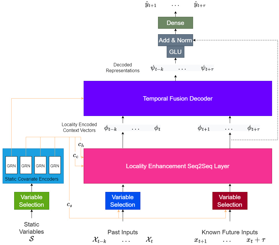
Figure 16.6 – TFT – a high-level overview

There is a lot to unpack here. Let’s start with the static variables, . First, the static variables are passed through a Variable Selection Network (VSN). The VSN does instance-wise feature selection and performs some non-linear processing on the inputs. This processed input is fed into a bunch of Static Covariate Encoders (SEs). The SE block is designed to integrate the static metadata in a principled way.

If you follow the arrows from the SE block in Figure 16.6, you will see that the static covariates are used in three (four distinct outputs) different places in the architecture. We will see how these are used in each of these places when we talk about them. But all these different places may be looking at different aspects of the static information. To allow the model this flexibility, the processed and variable-selected output is fed into four different Gated Residual Networks (GRNs), which, in turn, generate four outputs – , , , and . We will explain what a GRN is later, but for now, just understand that it is a block capable of non-linear processing, along with a residual connection, which enables it to bypass the non-linear processing if needed.

The past inputs, , and the future known inputs, , are also passed through separate VSNs and these processed outputs are fed into a Locality Enhancement (LE) Seq2Seq layer. We can think of LE as a way to encode the local context and temporal ordering into the embeddings of each timestep. This is similar to the positional embeddings in vanilla Transformers. We can also see similar attempts in the Conv1d layers that were used to encode the history in the uniform representation in the Informer and Autoformer models. We will see what is happening inside the LE later, but for now, just understand it captures the local context conditioned on other observed variables and static information. Let’s call the output of the block Locality Encoded Context Vectors (, and ).

Important note

The terminology, notation, and grouping of major blocks are not the same as in the original paper. I have changed these to make them more accessible and understandable.

Now, these LE context vectors are fed into a Temporal Fusion Decoder (TD). The TD applies a slight variation of multi-headed self-attention in a Transfomer model-like manner and produces the Decoded Representation (). Finally, this Decoded Representation is passed through a Gated Linear Unit (GLU) and an Add and Norm block that adds the LE context vectors as a residual connection.

A GLU is a unit that helps the model decide how much information it needs to allow to flow through. We can think of it as a learned information throttle that is widely used in Natural Language Processing (NLP) architectures. The formula is really simple:

Here, and are learnable weight matrices, and are learnable biases, is an activation function, and is the Hadamard product operator (element-wise multiplication).

The Add & Norm block is the same as in the vanilla Transformer; we discussed this back in Chapter 14, Attention and Transformers for Time Series.

Now, to top it all off, we have a Dense layer (linear layer with bias) that projects the output of the Add & Norm block to the desired output dimensions.

And with that, it is time for us to step one level down in our abstraction.

Locality Enhancement Seq2Seq layer

Let’s peel back the onion and see what’s happening inside the LE Seq2Seq layer. Let’s start with a figure:

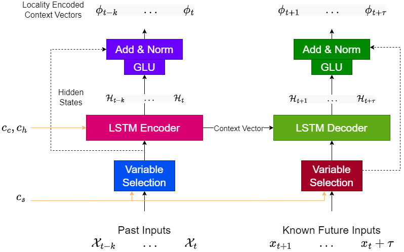
Figure 16.7 – TFT – LE Seq2Seq layer

The LE uses a Seq2Seq architecture to capture the local context. The process starts with the processed past inputs. The LSTM encoder takes in these past inputs, . ; from the static covariate encoder acts as the initial hidden states of the LSTM. The encoder processes each timestep at a time, producing hidden states at each time step, . The last hidden states (context vector) are now passed on to the LSTM decoder, which processes the known future inputs, , and produces the hidden states at each of the future timesteps, . Finally, all these hidden states are passed through a GLU + AddNorm block with the residual connection from before the LSTM processing. The outputs are the LE context vectors (, and .

Now, let’s look at the next block: the TFD.

Temporal fusion decoder

Let’s start this discussion with another figure:

Figure 16.8 – Temporal Fusion Transformer – Temporal Fusion Decoder

The LE context vectors from both the past input and known future input are concatenated into a single LE context vector. Now, this can be thought of as the position-encoded tokens in the Transformer paradigm. The first thing the TFD does is enrich these encodings with static information, , that was created from the static covariate encoder. This was concatenated with the embeddings. A position-wise GRN is used to enrich the embeddings. These enriched embeddings are now used as the query, key, and values for the Masked Interpretable Multi-Head Attention block.

The paper posits that the Masked Interpretable Multi-Head Attention block learns long-term dependencies across time steps. The local dependencies are already captured by the LE Seq2Seq layer in the embeddings, but the point-wise long-term dependencies are captured by Masked Interpretable Multi-Head Attention. This block also enhances the interpretability of the architecture. The attention weights that are generated in the process give us some indication of the major timesteps involved in the process. But the multi-head attention has one drawback from the interpretability perspective. In vanilla multi-head attention, we use separate projection weights for the values, which means that the values for each head are different and hence the attention weights are not straightforward to interpret.

TFT gets over this limitation by employing a single shared weight matrix for projecting the values into the attention dimension. Even with the shared value projection weights, because of the individual query and key projection weights, each head can learn different temporal patterns. In addition to this, TFT also employs masking to make sure information from the future is not used in operations. We discussed this type of causal masking in Chapter 14, Attention and Transformers for Time Series. With these two modifications, TFT names this layer Masked Interpretable Multi-Head Attention.

And with that, it’s time to open the last and most granular level of abstraction we have been using.

Gated Residual Network

We have been talking about GRNs for some time now; so far, we have just taken them at face value. Let’s understand what is happening inside a GRN – one of the most basic building blocks of a TFT.

Let’s look at a schematic diagram of a GRN to understand it better:

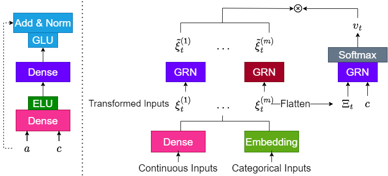
Figure 16.9 – TFT – GRN (left) and VSN (right)

The GRN takes in two inputs: the primary input, , and the external context, . The context, , is an optional input and is treated as zero if it’s not present. First, both the inputs, and , are transformed by separate dense layers and a subsequent activation function – the Exponential Linear Unit (ELU) (https://pytorch.org/docs/stable/generated/torch.nn.ELU.html).

Now, the transformed and inputs are added together and then transformed again using another Dense layer. Finally, this is passed through a GLU+Add & Norm layer with residual connections from the original . This structure bakes in enough non-linearity to learn complex interactions between the inputs, but at the same time lets the model ignore those non-linearities through a residual connection. Therefore, such a block allows the model to scale the computation required up or down based on the data.

Variable Selection Network

The last building block of the TFT is the VSN. VSNs enable TFT to do instance-wise variable selection. Most real-world time series datasets have many variables that do not have a lot of predictive power, so being able to select the ones that do have predictive power automatically will help the model pick out relevant patterns. Figure 16.9 (right) shows this VSN.

These additional variables can be categorical or continuous. TFT uses Entity Embeddings to convert the categorical features into numerical vectors of the dimension that we desire (). We talked about this in Chapter 15, Strategies for Global Deep Learning Forecasting Models. The continuous features are linearly transformed (independently) into the same dimension, . This gives us the Transformed inputs, , where is the number of features and is the timestep. We can concatenate all these embeddings (flatten them) and that flattened representation can be represented as .

Now, there are two parallel streams in which these embeddings are processed – one for non-linear processing of the embeddings and another to do feature selection. Each of these embeddings is processed by separate GRNs (but shared for all timesteps) to give us the non-linearly processed ones, . In another stream, the VSN processes the flattened representation, , along with optional context information, , and processes it through a GRN with a softmax activation. This gives us a weight, , which is a vector of length . This is now used in a weighted sum of all the non-linearly processed feature embeddings, , which is calculated as follows:

Forecasting with TFT

TFT is implemented in PyTorch Forecasting. We can use the same framework we worked with in Chapter 15, Strategies for Global Deep Learning Forecasting Models, and extend it to train TFT on our data.

The TemporalFusionTransformer class in PyTorch Forecasting has the following major parameters:

• hidden_size: This is an integer representing the hidden dimension across the model. This is the dimension in which all the GRNs work, the VSN, the LSTM hidden sizes, the self-attention hidden sizes, and so on. Arguably, this is the most important hyperparameter in the model.
• lstm_layers: This is an integer that determines the number of layers in the LSTMs we use in the LE Seq2Seq block.
• attention_head_size: This is an integer representing the number of attention heads.
• embedding_sizes: This is a dictionary of categorical feature names to a tuple of (cardinality, embedding size). Although the original paper suggests projecting all categorical and continuous variables to a single dimension, the PyTorch Forecasting implementation allows the flexibility to have separate dimensions for each variable.
• hidden_continuous_size: This is an integer that is the default embedding size for continuous features.
• hidden_continuous_sizes: This is a dictionary of continuous feature names to a hidden size for variable selection. This lets us override hidden_continuous_size for specific features.
• dropout: This is a float between 0 and 1, which determines the strength of the dropout in the network.

Notebook alert

The complete code for training TFT can be found in the 05-TFT.ipynb notebook in the Chapter16 folder. There are two variables in the notebook that act as switches – TRAIN_SUBSAMPLE = True makes the notebook run for a subset of 10 households, while train_model = True makes the notebook train different models (warning: training the model on the full data takes hours). train_model = False loads the trained model weights (not included in the repository but saved every time you run training) and predicts on them.

Interpreting TFT

TFT approaches interpretability from a slightly different perspective than N-BEATS. While N-BEATS gives us a decomposed output for interpretability, TFT gives us visibility into how the model has interpreted the variables it has used. On account of the VSNs, we have ready access to feature weights. Like the feature importance we get from tree-based models, TFT gives us access to similar scores. And because of the self-attention layer, the attention weights can also be interpreted to help us understand which time steps hold a large enough weightage in the attention mechanism.

PyTorch Forecasting makes this possible by performing a few steps. First, we get the raw predictions using mode="raw" in the predict function. Then, we use those raw predictions in the interpret_output function. There is a parameter called reduction in the interpret_output function that decides how to aggregate the weights across different instances. We know that TFT does instance-wise feature selection in VSNs and attention is also done instance-wise. 'mean' is a good option for looking at the global interpretability:

raw_predictions, x = best_model.predict(val_dataloader, mode="raw", return_x=True)
interpretation = best_model.interpret_output(raw_predictions, reduction="sum")

This interpretation variable is a dictionary with weights for different aspects of the model, such as attention, static_variables, encoder_variables, and decoder_variables. PyTorch Forecasting also provides us with an easy way to visualize this importance:

best_model.plot_interpretation(interpretation)

This generates four plots:

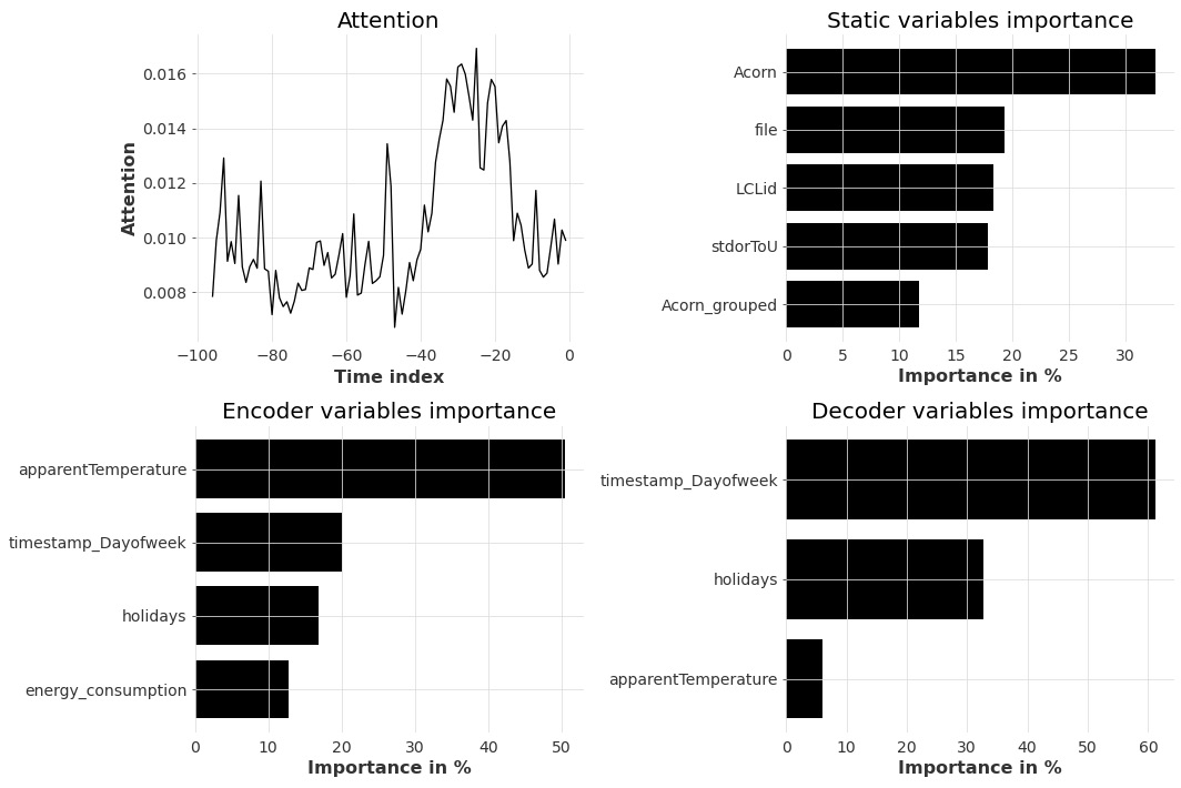
Figure 16.10 – Interpreting TFT

We can also look at each instance and plot similar visualizations for each prediction we make. All we need to do is use reduction="none" and then plot it ourselves. The accompanying notebook explores how to do that and more.

We have covered a few popular specialized architectures for time series forecasting, but this is in no way a complete list. There are so many model architectures and techniques out there. I have included a few in the Further reading section to get you started.

Interpretability

I directed you toward a few interpretability techniques for machine learning models back in Chapter 10, Global Forecasting Models. While some of those, such as SHAP and LIME, can still be applied to deep learning models, none of them considers the temporal aspect by design. This is because all those techniques were developed for more general purposes, such as classification and regression. That being said, there has been some work in interpretability for DL models and time series models. Here, I’ll list a few promising papers that tackle the temporal aspect head-on:

• TimeSHAP: This is a model-agnostic recurrent explainer that builds upon KernelSHAP and extends it to the time series domain. Research paper: https://dl.acm.org/doi/10.1145/3447548.3467166. GitHub: https://github.com/feedzai/timeshap.
• Instance-wise Feature Importance in Time (FIT): This is an interpretability technique that relies on the distribution shift between the predictive distribution and a counterfactual where all but the feature under inspection are unobserved. Research paper: https://proceedings.neurips.cc/paper/2020/file/08fa43588c2571ade19bc0fa5936e028-Paper.pdf. GitHub: https://github.com/sanatonek/time_series_explainability.
• Dynamask - Explaining Time Series Predictions with Dynamic Masks: A technique that produces instance-wise importance scores for each feature at each time step by fitting a perturbation mask to the input sequence. Research paper: http://proceedings.mlr.press/v139/crabbe21a.html. GitHub: https://github.com/JonathanCrabbe/Dynamask.

While this is not an exhaustive list, these are a few works that I feel are important and promising. This is an area of active research and new techniques will come up as time goes on.

Now, let’s take a look at another aspect, although not a specialized architecture, but a key component that can elevate the forecasts you generate to another dimension.

Probabilistic forecasting

So far, we have been talking about the forecast as a single number. We have been projecting our DL models to a single dimension and training the model using a loss such as mean squared loss. This paradigm is what we call a point forecast. A probabilistic forecast is when the forecast, instead of having a single-point prediction, captures the uncertainty of that forecast as well. This means that the model doesn’t output a single number, but an output that reflects the probabilities associated with all possible future outcomes.

In the econometrics and classical time series world, the prediction intervals were already baked into the formulation. The statistical grounding of those methods made sure that the output of those models was readily interpreted in a probabilistic way as well (so long as you could satisfy the assumptions that were stipulated by those models). But in the modern machine/DL world, probabilistic forecasting is not an afterthought. A combination of factors such as less rigid assumptions and the way we train the models leads to this predicament.

From a probabilistic point of view, a forecast at position , , can be seen as the realization of a probability distribution, . And instead of estimating , the model estimates . There are a few popular ways in DL to estimate . Let’s look at them one by one.

Probability Density Function (PDF)

This is the most common way of representing probability distribution in forecasting. Standard parametric probability distributions have a few parameters that define the full distribution. For instance, the Gaussian distribution can be fully parameterized by the mean and the standard deviation. So, if we assume that the forecast is from one of these parametric distributions, we can tweak the model so that it outputs the parameters of the distribution, rather than a single-point estimate. For instance, the final projection to the output space of a DL model can be tweaked to output two parameters – the mean, , and the standard deviation, , at time . There are specific constraints to these outputs that are typically handled by the right activation function. For instance, should be a positive number because a negative standard deviation doesn’t make sense. So, we can apply an activation function, such as a ReLU or a SoftPlus function, to make sure those considerations are met.

Now that the model has two outputs, the mean and standard deviation, we also need to change the loss function. It is not as if the target that we are training the model with is in PDF form. In other words, the targets are still real numbers and not means and standard deviations. So, instead of a loss function such as mean squared error, we need to use something such as a negative log-likelihood (NLL). Let’s understand this a bit more.

For instance, let’s say you have a set of iid observations (in our case, the target), . With PDF, we will be able to tell the probability of each of those observations, . From high school probability, we know that when two independent events occur, to get the joint probability, we can just multiply them together. Using the same logic, to calculate the joint probability of all n iid observations (the probability that all of them occur), we can just multiply all of them together:

However, this operation is not numerically stable – if you start multiplying numbers less than zero, it gets smaller and smaller and eventually leads to numerical underflow. Therefore, a more stable version of the same likelihood is used – log-likelihood. Optimizing a function and a log of the same function is synonymous. By using the log, the series of multiplications becomes an addition and instantly more stable:

So, all we need is to plug into the NLL loss. This comes from our assumption regarding the distribution the output will be in and the estimated parameters of the model. This allows the model to compute the likelihood that a particular point (the target) is under the predicted distribution and then minimize the NLL (or maximize the likelihood) by changing the model parameters.

Apart from the Gaussian assumption, several differentiable parametric distributions have been used by different researchers for forecasting problems – student-t distribution, Tweedie distribution, negative binomial distribution, and so on. DeepAR by Salinas et al. is a prominent example where this approach has been used to great success.

Reference check

The research paper by Salinas et al. on DeepAR is cited in the References section as 11.

Quantile functions

Another way can be represented is by using quantile functions. Before talking about the quantile function, let’s spend a minute on the Cumulative Distribution Function (CDF). This, again, is high school probability. In simple words, a CDF returns the probability of some random variable, , being less than or equal to some value, :

Here, is the CDF. This function takes in an input, , and returns a value between 0 and 1. Let’s call this value .

A quantile function is an inverse of the CDF. This function tells you the value of x, which would make F(x) return a particular value, :

This function, , is the quantile function. Similar to the PDF, the quantile function also provides a complete description of the distribution. Therefore, repurposing the model to learn the quantile function for specific quantiles that are of interest to us also gives us probabilistic forecasts.

From an implementation perspective, we would have to choose quantiles we want to estimate (0.1, 0.5, and 0.9 are popular choices) and tweak the last layer that projects to the output space so that there are outputs. In this case, the most common choice for a loss function is the Quantile Loss or the Pinball Loss.

The Quantile Loss can be defined as follows:

Here, is the target value at time t, is the quantile forecast, and is the quantile we are forecasting. While implementing this, we can easily replace the branched equation with a maximum operation:

def quantile_loss(q, y, y_hat_q):
  # q: Quantile to be evaluated, e.g., 0.5 for median.
  # y: Target Value
  # y_hat_q: Quantile Forecast.
  e = y - f
  return np.maximum(q * e, (q - 1) * e)

Typically, we train with multiple quantiles. In this case, the loss the model optimizes for will be the sum of all the quantile loss for each of the quantiles we are training for.

TFTs are a great example where uncertainty quantification is done using a quantile function. The paper originally proposed TFT as a probabilistic forecasting option. For a more detailed explanation of quantile loss, head over to the Further reading section.

Other approaches

Apart from PDF and quantile functions, there are a lot of other approaches to probabilistic forecasting. We will not be able to cover all of them here, but I will still try to mention the major ones and give you references so that you can read more about the technique:

• Monte Carlo dropout: This trick only works for networks with dropout. Dropouts are generally turned off while inferencing. However, in Monte Carlo dropout, we keep the dropout on and predict multiple times. This approximates Bayesian computation and estimates model uncertainty. A popular research paper implementing this idea for time series is Deep and Confident Prediction for Time Series at Uber by Zhu et al. at https://doi.org/10.1109/ICDMW.2017.19.
• Normalizing flows: Normalizing flows are a method for learning complex data distributions by transforming a simple distribution into a complex distribution. They do this by learning a series of invertible and differentiable functions, such that we have a one-to-one correspondence between points in the simple distribution to points in the complex distribution. Therefore, we can have a bijective function (a function mapping between domain A to domain B such that for every element, b, in B, there is exactly one element, a, in A) that maps the data distribution (complex) to a simple distribution (such as a Gaussian distribution). A recent paper that applies normalizing flows to multivariate time series forecasting is Multivariate Probabilistic Time Series Forecasting via Conditioned Normalizing Flows by Rasul et al. This was presented in ICLR 2021 and can be accessed at https://openreview.net/forum?id=WiGQBFuVRv.
• Conformal prediction: Conformal prediction is an increasingly popular way to create distribution-free prediction intervals. It uses a trained model’s experience in past data (calibration data) to recalibrate the confidence in new predictions. There is a large body of work and it is a very rapidly advancing field. I’m citing an example where the authors apply conformal predictions to a time series setting. For more information, you can refer to Conformal Time-series Forecasting by Stankeviciute et al., which was presented at NeurIPS 2021 and is accessible at https://proceedings.neurips.cc/paper/2021/hash/312f1ba2a72318edaaa995a67835fad5-Abstract.html.

Congratulations on making it through probably, one of the toughest and densest chapters in this book. Give yourself a pat on the back, sit back, and relax.

Summary

Our journey with deep learning for time series has finally reached a conclusion with us reviewing a few specialized architectures for time series forecasting. We now understand how different models such as N-BEATS, N-BEATSx, N-HiTS, Informer, Autoformer, and TFT work.

We also looked at how we can apply those models using PyTorch Forecasting. For the models such as Informer and Autoformer that were not implemented in PyTorch Forecasting, we saw how we can port normal PyTorch models into a form that can be used with PyTorch Forecasting. Models such as N-BEATS and TFT also offer interpretability and we explored those use cases as well.

To top this off, we covered probabilistic forecasting at a high level and provided references so that you can start your journey of looking at them. This brings this part of this book to a close. At this point, you should be much more comfortable with using DL for time series forecasting problems.

In the next part of this book, we will look at a few mechanics of forecasting, such as multi-step forecasting, cross-validation, and evaluation.

References

The following is a list of the references that we used throughout this chapter:

1. Spyros Makridakis, Evangelos Spiliotis, and Vassilios Assimakopoulos. (2020). The M4 Competition: 100,000 time series and 61 forecasting methods. International Journal of Forecasting, Volume 36, Issue 1. Pages 54-74. https://doi.org/10.1016/j.ijforecast.2019.04.014.
2. Slawek Smyl. (2018). M4 Forecasting Competition: Introducing a New Hybrid ES-RNN Model. https://www.uber.com/blog/m4-forecasting-competition/.
3. Boris N. Oreshkin, Dmitri Carpov, Nicolas Chapados, and Yoshua Bengio. (2020). N-BEATS: Neural basis expansion analysis for interpretable time series forecasting. 8th International Conference on Learning Representations, (ICLR). https://openreview.net/forum?id=r1ecqn4YwB.
4. Kin G. Olivares and Cristian Challu and Grzegorz Marcjasz and R. Weron and A. Dubrawski. (2022). Neural basis expansion analysis with exogenous variables: Forecasting electricity prices with NBEATSx. International Journal of Forecasting, 2022. https://www.sciencedirect.com/science/article/pii/S0169207022000413.
5. Cristian Challu and Kin G. Olivares and Boris N. Oreshkin and Federico Garza and Max Mergenthaler-Canseco and Artur Dubrawski. (2022). N-HiTS: Neural Hierarchical Interpolation for Time Series Forecasting. arXiv preprint arXiv: Arxiv-2201.12886. https://arxiv.org/abs/2201.12886.
6. Vaswani, Ashish, Shazeer, Noam, Parmar, Niki, Uszkoreit, Jakob, Jones, Llion, Gomez, Aidan N, Kaiser, Lukasz, and Polosukhin, Illia. (2017). Attention is All you Need. Advances in Neural Information Processing Systems. https://papers.nips.cc/paper/2017/hash/3f5ee243547dee91fbd053c1c4a845aa-Abstract.html.
7. Yao-Hung Hubert Tsai, Shaojie Bai, Makoto Yamada, Louis-Philippe Morency, and Ruslan Salakhutdinov. (2019). Transformer Dissection: An Unified Understanding for Transformer’s Attention via the Lens of Kernel. N Proceedings of the 2019 Conference on Empirical Methods in Natural Language Processing and the 9th International Joint Conference on Natural Language Processing (EMNLP-IJCNLP), pages 4,344–4,353. https://aclanthology.org/D19-1443/.
8. Haoyi Zhou, Shanghang Zhang, Jieqi Peng, Shuai Zhang, Jianxin Li, Hui Xiong, and Wancai Zhang. (2021). Informer: Beyond Efficient Transformer for Long Sequence Time-Series Forecasting. Thirty-Fifth {AAAI} Conference on Artificial Intelligence, {AAAI} 2021. https://ojs.aaai.org/index.php/AAAI/article/view/17325.
9. Haixu Wu, Jiehui Xu, Jianmin Wang, and Mingsheng Long. (2021). Autoformer: Decomposition Transformers with Auto-Correlation for Long-Term Series Forecasting. Advances in Neural Information Processing Systems 34: Annual Conference on Neural Information Processing Systems 2021, NeurIPS 2021, December 6-14, 2021. https://proceedings.neurips.cc/paper/2021/hash/bcc0d400288793e8bdcd7c19a8ac0c2b-Abstract.html.
10. Bryan Lim, Sercan Ö. Arik, Nicolas Loeff, and Tomas Pfister. (2019). Temporal Fusion Transformers for Interpretable Multi-horizon Time Series Forecasting. International Journal of Forecasting, Volume 37, Issue 4, 2021, Pages 1,748-1,764. https://www.sciencedirect.com/science/article/pii/S0169207021000637.
11. David Salinas, Valentin Flunkert, and Jan Gasthaus. (2017). DeepAR: Probabilistic Forecasting with Autoregressive Recurrent Networks. International Journal of Forecasting, 2017. https://www.sciencedirect.com/science/article/pii/S0169207019301888.

Further reading

You can check out the following resources for further reading:

• Fast ES-RNN: A GPU Implementation of the ES-RNN Algorithm: https://arxiv.org/abs/1907.03329 and https://github.com/damitkwr/ESRNN-GPU
• Functions as Vector Spaces: https://www.youtube.com/watch?v=NvEZol2Q8rs
• Forecast with N-BEATS, by Gaetan Dubuc: https://www.kaggle.com/code/gatandubuc/forecast-with-n-beats-interpretable-model/notebook
• WaveNet: A Generative Model for Audio, by DeepMind: https://www.deepmind.com/blog/wavenet-a-generative-model-for-raw-audio
• What is Residual Connection?, by Wanshun Wong: https://towardsdatascience.com/what-is-residual-connection-efb07cab0d55
• Efficient Transformers: A Survey, by Tay et al.: https://arxiv.org/abs/2009.06732
• Autocorrelation and the Wiener-Khinchin theorem: https://www.itp.tu-berlin.de/fileadmin/a3233/grk/pototskyLectures2012/pototsky_lectures_part1.pdf
• Modelling Long- and Short-Term Temporal Patterns with Deep Neural Networks, by Lai et al.: https://dl.acm.org/doi/10.1145/3209978.3210006 and https://github.com/cure-lab/SCINet.
• Think Globally, Act Locally: A Deep Neural Network Approach to High-Dimensional Time Series Forecasting, by Sen et al.: https://proceedings.neurips.cc/paper/2019/hash/3a0844cee4fcf57de0c71e9ad3035478-Abstract.html and https://github.com/rajatsen91/deepglo
• Enhancing the Locality and Breaking the Memory Bottleneck of Transformer on Time Series Forecasting, by Li et al.: https://proceedings.neurips.cc/paper/2019/hash/6775a0635c302542da2c32aa19d86be0-Abstract.html
• Quantile loss function for machine learning, by Evergreen Innovations: https://www.evergreeninnovations.co/blog-quantile-loss-function-for-machine-learning/