
13
Common Modeling Patterns for Time Series
We reviewed a few major and common building blocks of a deep learning (DL) system, specifically suited for time series, in the last chapter. Now that we know what those blocks are, it’s time for a more practical lesson. Let’s see how we can put these common blocks together in various common ways in which time series forecasting is modeled using the dataset we have been working with all through this book.
In this chapter, we will be covering these main topics:
- Tabular regression
- Single-step-ahead recurrent neural networks
- Sequence-to-sequence models
Technical requirements
You will need to set up the Anaconda environment following the instructions in the Preface of the book to get a working environment with all packages and datasets required for the code in this book.
The associated code for the chapter can be found at https://github.com/PacktPublishing/Modern-Time-Series-Forecasting-with-Python-/tree/main/notebooks/Chapter13.
You need to run the following notebooks for this chapter:
- 02-Preprocessing London Smart Meter Dataset.ipynb in Chapter02
- 01-Setting up Experiment Harness.ipynb in Chapter04
- 01-Feature Engineering.ipynb in Chapter06
- 00-Single Step Backtesting Baselines.ipynb, 01-Forecasting with ML.ipynb, and 02-Forecasting with Target Transformation.ipynb in Chapter08
- 01-Global Forecasting Models-ML.ipynb in Chapter10
Tabular regression
In Chapter 5, Time Series Forecasting as Regression, we saw how we can convert a time series problem into a standard regression problem by temporal embedding and time delay embedding. In Chapter 6, Feature Engineering for Time Series Forecasting, we have already created the necessary features for the household energy consumption dataset we have been working on, and in Chapter 8, Forecasting Time Series with Machine Learning Models, Chapter 9, Ensembling and Stacking, and Chapter 10, Global Forecasting Models, we used traditional machine learning (ML) models to create a forecast.
Just as we used standard ML models for forecasting, we can also use DL models built for tabular data using the feature-engineered dataset we have created. One of the advantages of using a DL model in this setting, over the ML models, is the flexibility DL offers us. All through Chapters 8, 9, and 10, we only saw how we can create single-step-ahead forecasting using ML models. We have a separate section on multi-step forecasting in Part 3, Deep Learning for Time Series, where we go into detail on different strategies with which we can generate multi-step forecasts, and we address one of the limitations of standard ML models in multi-step forecasting. But right now, let’s just understand that standard ML models are designed to have a single output and, because of that fact, getting multi-step forecasts is not straightforward. But with tabular DL models, we have the flexibility to train the model to predict multiple targets, and this enables us to generate multi-step forecasts easily.
PyTorch Tabular is an open source library (https://github.com/manujosephv/pytorch_tabular) that makes it easy to work with DL models in the tabular data domain, and it also has ready-to-use implementations of many state-of-the-art DL models. We are going to use PyTorch Tabular to generate forecasts using the feature-engineered datasets we created in Chapter 6, Feature Engineering for Time Series Forecasting.
PyTorch Tabular has very detailed documentation and tutorials to get you started here: https://pytorch-tabular.readthedocs.io/en/latest/. Although we won’t be going into detail on all the intricacies of the library, we will look at how we can use a bare-bones version to generate a forecast on the dataset we are working on using a FTTransformer model. FTTransformer is one of the state-of-the-art DL models for tabular data. DL for tabular data is a whole different kind of model, and I’ve linked a blog post in the Further reading section as a primer to the field of study. For our purposes, we can treat them as any standard ML model in scikit-learn.
Notebook alert
To follow along with the complete code, use the notebook named 01-Tabular Regression.ipynb in the Chapter13 folder and the code in the src folder.
We start off, pretty much like before, by loading the libraries and necessary datasets. Just one additional thing we are doing here is that instead of taking the same selection of blocks we worked with in Part 2, Machine Learning for Time Series, we take smaller-sized data by selecting half the number of blocks as before. This is done to make the neural network (NN) training smoother and faster and for it to fit into GPU memory (if any). I’d like to stress here that this is done purely for hardware reasons, and provided we have sufficiently powerful hardware, we need not have smaller datasets for DP. On the contrary—DL loves larger datasets. But since we want to keep the focus on the modeling side, the engineering constraints and techniques in working with larger datasets have been kept outside the scope of this book.
uniq_blocks = train_df.file.unique().tolist()
sel_blocks = sorted(uniq_blocks, key=lambda x: int(x.replace("block_","")))[:len(uniq_blocks)//2]
train_df = train_df.loc[train_df.file.isin(sel_blocks)]
test_df = test_df.loc[test_df.file.isin(sel_blocks)]
sel_lclids = train_df.LCLid.unique().tolist()
After handling the missing values, we are ready to start using PyTorch Tabular. We first import the necessary classes from the library, like so:
from pytorch_tabular.config import DataConfig, OptimizerConfig, TrainerConfig
from pytorch_tabular.models import FTTransformerConfig
from pytorch_tabular import TabularModel
PyTorch Tabular uses a set of config files to define the parameters required for running the model, and these configs include everything from how the dataframe is configured to what kind of preprocessing needs to be applied, what kind of training we need to do, what model we need to use, what the hyperparameters of the model are, and so on. Let’s see how we can define a bare-bones configuration (because PyTorch Tabular makes use of intelligent defaults wherever possible to make the usage easier for the practitioner):
data_config = DataConfig(
    target=[target], #target should always be a list
    continuous_cols=[
        "visibility",
        "windBearing",
        …
        "timestamp_Is_month_start",
    ],
    categorical_cols=[
        "holidays",
        …
        "LCLid"
    ],
    normalize_continuous_features=True
)
trainer_config = TrainerConfig(
    auto_lr_find=True, # Runs the LRFinder to automatically derive a learning rate
    batch_size=1024,
    max_epochs=1000,
    auto_select_gpus=True,
    gpus=-1
)
optimizer_config = OptimizerConfig()
We use a very high max_epochs parameter in TrainerConfig because by default, PyTorch Tabular employs a technique called early stopping, where we continuously keep track of the performance on a validation set and stop the training when the validation loss starts to increase.
Selecting which model to use from the implemented models in PyTorch Tabular is as simple as choosing the right configuration. Each model is associated with a configuration that defines the hyperparameters of the model. So, just by using that specific configuration, PyTorch Tabular understands which model the user wants to use. Let’s choose the FTTransformerConfig model and define a few hyperparameters:
model_config = FTTransformerConfig(
    task="regression",
    num_attn_blocks=3,
    num_heads=4,
    transformer_head_dim=64,
    attn_dropout=0.2,
    ff_dropout=0.1,
    out_ff_layers="32",
    metrics=["mean_squared_error"]
)
The main and only mandatory parameter here is task, which tells PyTorch Tabular whether it is a regression or classification task.
Additional note
Although PyTorch Tabular provides the best defaults, we only set these parameters to make the training faster and fit into the memory of the GPU we are running on. If you are not running the notebook on a machine with a GPU, choosing a smaller and faster model such as CategoryEmbeddingConfig would be better.
Now, all that is left to do is put all these configs together in a class called TabularModel, which is the workhorse of the library, and as with any scikit-learn model, call fit on the object. But, unlike a scikit-learn model, you don’t need to split X and y; we just need to provide the dataframe, as follows:
tabular_model.fit(train=train_df)
Once the training completes, you can save the model by just running the following code:
tabular_model.save_model("notebooks/Chapter13/ft_transformer_global")If for any reason you have to close your notebook instance after training, you can always load the model back by using the following code:
tabular_model = TabularModel.load_from_checkpoint("notebooks/Chapter13/ft_transformer_global")This way, you don’t need to spend a lot of time training the model again, but instead, use it for prediction.
Now, all that is left is to predict on the unseen data and evaluate the performance. Here’s how we can do this:
forecast_df = tabular_model.predict(test_df)
agg_metrics, eval_metrics_df = evaluate_forecast(
    y_pred=forecast_df[f"{target}_prediction"],
    test_target=forecast_df["energy_consumption"],
    train_target=train_df["energy_consumption"],
    model_name=model_config._model_name,
)
We have used the untuned global forecasting model with metadata that we trained in Chapter 10, Global Forecasting Models, as the baseline against which we can do a cursory check on how well the DL model is doing, as illustrated in the following screenshot:
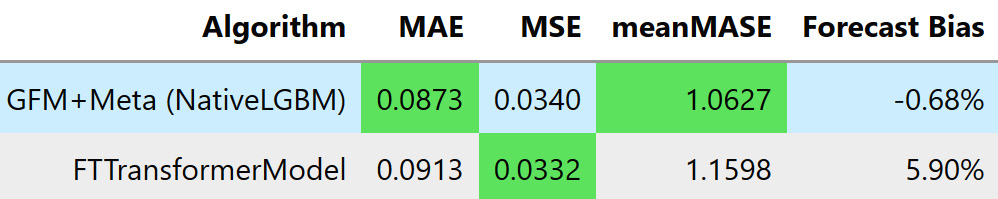
Figure 13.1 – Evaluation of the DL-based tabular regression
We can see that the FTTransformer model is competitive with the LightGBM model we trained in Chapter 10. Maybe, with the right amount of tuning and partitioning, the FTTransformer model can do as well or better than the LightGBM one. Training a competitive DL model in the same way as LightGBM is useful in many ways. First, this brings us flexibility and trains the model to predict multiple timesteps at once. Second, this can also be combined with the LightGBM model in an ensemble, and because of the variety the DL model brings to the mix, this can make the ensemble performance better.
Things to try
Use PyTorch Tabular’s documentation and play around with other models or change the parameters to see how the performances changes.
Select a few households and plot them to see how well the forecast matches up to the targets.
Now, let’s look at how we can use RNN for single-step-ahead forecasting.
Single-step-ahead recurrent neural networks
Although we took a little detour to check out how DL regression models can be used to train the same global models we learned about in Chapter 10, Global Forecasting Models, now we are back to looking at DL models and architectures specifically built for time series. And as always, we will look at simple one-step-ahead and local models first before moving on to more complex modeling paradigms. In fact, we have another chapter (Chapter 15, Strategies for Global Deep Learning Forecasting Models) entirely devoted to techniques we can use to train global DL models.
Now, let’s bring our attention back to one-step-ahead local models. We saw recurrent neural networks (RNNs) (vanilla RNN, long short-term memory (LSTM), and gated recurrent unit (GRU)) as a few blocks we can use for sequences such as time series. Now, let’s see how we can use them in an end-to-end (E2E) model on the dataset we have been working on (the London smart meters dataset).
Although we will be looking at a few libraries (such as darts) that make the process of training DL models for time series forecasting easier, in this chapter, we will be looking at how to develop such models from scratch. Understanding how a DL model for time series forecasting is put together from the ground up will give you a good grasp of the concepts that are needed to use and tweak the libraries that we will be looking at later.
We will be using PyTorch, and if you are not comfortable, I suggest you head to Chapter 12, Building Blocks of Deep Learning for Time Series, and the associated notebooks for a quick refresher. On top of that, we are also going to use PyTorch Lightning, which is another library built on top of PyTorch to make training models using PyTorch easy, among other benefits.
We talked about time delay embedding in Chapter 5, Time Series Forecasting as Regression, where we talked about using a window in time to embed the time series into a format more suitable for regression. When training NNs for time series forecasting also, we need such windows. Suppose we are training on a single time series. We can give this super long time series to an RNN as is, but then it only becomes one sample in the dataset. And with just one sample in the dataset, it’s close to impossible to train any ML or DL models. So, it’s advisable to sample multiple windows from the time series to convert the time series into a number of data samples in a process that is very much similar to time delay embedding. This window also sets the memory of the DL model.
The first step we need to take is to create a PyTorch dataset that takes the raw time series and prepares these samples’ windows. A dataset is like an iterator over the data that gives us samples corresponding to a provided index. Defining a custom dataset for PyTorch is as simple as defining a class that takes in a few arguments (data being one of them) and defining two mandatory methods in the class, as follows:
- __len__(self)—This sets the maximum number of samples in the dataset.
- __get_item__(self, idx)—This picks the idxth sample from the dataset.
We have defined a dataset in src/dl/dataloaders.py with the name TimeSeriesDataset, which takes in the following parameters:
- data—This argument can either be a pandas dataframe or a NumPy array with the time series. This is the entire time series, including train, validation, and test, and the splits occur inside the class.
- window—This sets the length of each sample.
- horizon—This sets the number of future timesteps we want to get as the target.
- n_val—This parameter can either be a float or an int data type. If int, it represents the number of timesteps to be reserved as validation data. And if float, this represents the percent of total data to be reserved as validation data.
- n_test—This parameter is similar to n_val, but does the same for test data.
- normalize—This parameter defines how we want to normalize the data. This takes in three options: none means no normalizing; global means we calculate the mean and standard deviation of the train data and use it to standardize the entire series using this equation:

local means we use the window mean and standard deviation to standardize the series.
- normalize_params—This parameter takes in a tuple of mean and standard deviations. If provided, this is be used to standardize in global standardization. This is typically used to use the train mean and standard deviation on validation and test data as well.
- mode—This parameter sets which dataset we want to make. It takes in one of three values: train, val, or test.
Each sample from this dataset returns to you two tensors—the window (X) and the corresponding target (Y) (see Figure 13.2):
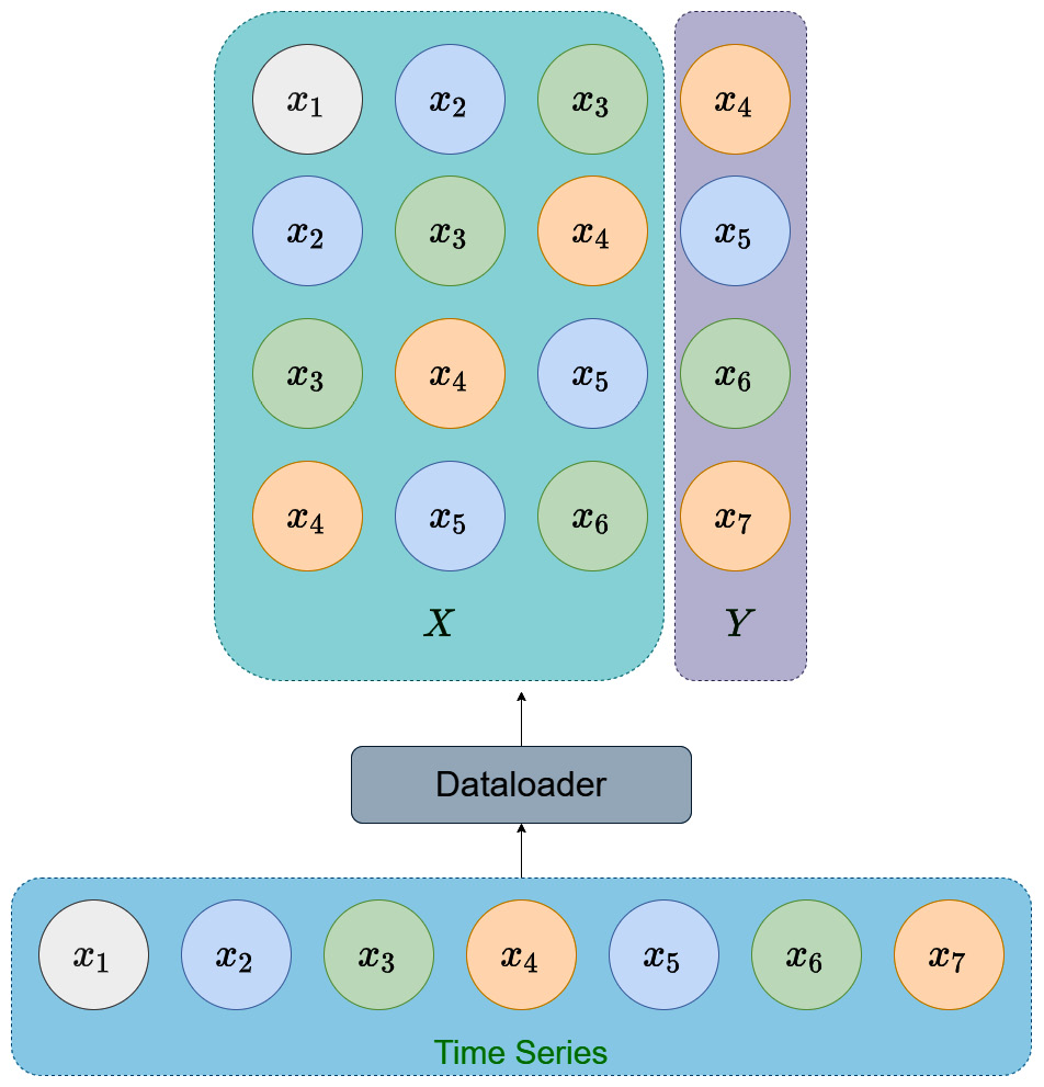
Figure 13.2 – Sampling the time series using a dataset and dataloader
Now that we have the dataset defined, we need another PyTorch artifact called a dataloader. A dataloader uses the dataset to pick samples into a batch of samples, among other things. In the PyTorch Lightning ecosystem, we have another concept called a datamodule, which is a standard way of generating dataloaders. We need train dataloaders, validation dataloaders, and test dataloaders. Datamodules provide a good abstraction to encapsulate the whole data part of the pipeline. We have defined a datamodule in src/dl/dataloaders.py called TimeSeriesDataModule that takes in the data along with the batch size and prepares the datasets and dataloaders necessary for training. The parameters are exactly the same as TimeSeriesDataset, with batch_size as the only additional parameter.
Notebook alert
To follow along with the complete code, use the notebook named 02-One-Step RNN.ipynb in the Chapter13 folder and the code in the src folder.
We will not be going into each and every step in the notebook but will be just stressing the key points. The code in the notebook is well commented, and we urge you to follow the code along with the book.
We have already sampled a household from the data, and now, let’s see how we can define a datamodule:
datamodule = TimeSeriesDataModule(data = sample_df[[target]],
        n_val = sample_val_df.shape[0],
        n_test = sample_test_df.shape[0],
        window = 48, # giving enough memory to capture daily seasonality
        horizon = 1, # single step
        normalize = "global", # normalizing the data
        batch_size = 32,
        num_workers = 0)
datamodule.setup()
datamodule.setup() is the method that calculates and sets up the dataloaders. Now, we can access the train dataloader by simply calling datamodule.train_dataloader(), and similarly, validation and test by val_dataloader and test_dataloader methods, respectively. And we can access the samples, as follows:
# Getting a batch from the train_dataloader
for batch in datamodule.train_dataloader():
    x, y = batch
    break
print("Shape of x: ",x.shape) #-> torch.Size([32, 48, 1])
print("Shape of y: ",y.shape) #-> torch.Size([32, 1, 1])
We can see that each sample has two tensors—x and y. There are three dimensions for the tensors, and they correspond to batch size, sequence length, features.
Now that we have the data pipeline ready, we need to build out the modeling and training pipelines. PyTorch Lightning has a standard way of defining these so that they can be plugged into the training engine they provide (which makes our life so much easier). The PyTorch Lightning documentation (https://pytorch-lightning.readthedocs.io/en/latest/starter/introduction.html) has good resources to get started with and go into depth on as well. We have also linked to a video in the Further reading section that makes the transition from pure PyTorch to PyTorch Lightning easy. I strongly urge you to take some time to familiarize yourself with it.
If you are familiar with standard PyTorch, you’ll know that a standard method called forward is the only mandatory method you have to define, apart from __init__. This is because the training loop is something that we will have to write on our own. In the 01-PyTorch Basics.ipynb notebook for Chapter 12, Building Blocks of Deep Learning for Time Series, we saw how we can write a PyTorch model and a training loop to train a simple classifier. But now that we are delegating the training loop to PyTorch Lightning, we have to include a few additional methods as well:
- training_step—This method takes in a batch and uses the model to get the outputs, calculate the loss/metrics, and return the loss.
- validation_step and test_step—These methods take in the batch and use the model to get the outputs and calculate the loss/metrics.
- predict_step—This method is used to define the step to be taken while inferencing. If there is anything special we have to do for inferencing, we can define this method. If this is not defined, it uses test_step for the prediction use case as well.
- configure_optimizers—This method defines the optimizer to be used; for instance, Adam, RMSProp, and so on.
We have defined a BaseModel class in src/dl/models.py that implements all the common functions, such as loss and metric calculation, logging of results, and so on, as a framework to implement new models. And using this BaseModel class, we have defined a SingleStepRNNModel class that takes in a standard config (SingleStepRNNConfig) and initializes an RNN, LSTM, or GRU model.
Before we look at how the model is defined, let’s see what the different config (SingleStepRNNConfig) parameters are:
- rnn_type—This parameter takes in one of three strings as an input: RNN, GRU, or LSTM. This defines what kind of model we will initialize.
- input_size—This parameter defines the number of features the RNN is expecting.
- hidden_size, num_layers, bidirectional—These parameters are the same as the ones we saw in the RNN cell in Chapter 12, Building Blocks of Deep Learning for Time Series.
- learning_rate—This defines the learning rate of the optimization procedure.
- optimizer_params, lr_scheduler, lr_scheduler_params—These are parameters that let us tweak the optimization procedure. Let’s not worry about these for now because all of them have been set to intelligent defaults.
With this setup, defining a new model is as simple as this:
rnn_config = SingleStepRNNConfig(
    rnn_type="RNN",
    input_size=1,
    hidden_size=128,
    num_layers=3,
    bidirectional=True,
    learning_rate=1e-3,
    seed=42,
)
model = SingleStepRNNModel(rnn_config)
Now, let’s take a peek at the forward method, which is the heart of the model. We want our model to do one-step-ahead prediction, and from Chapter 12, Building Blocks of Deep Learning for Time Series, we know what a typical RNN output is and how PyTorch RNNs just output the hidden state at each timestep. Let’s see what we want to do visually and then see how we can code it up:
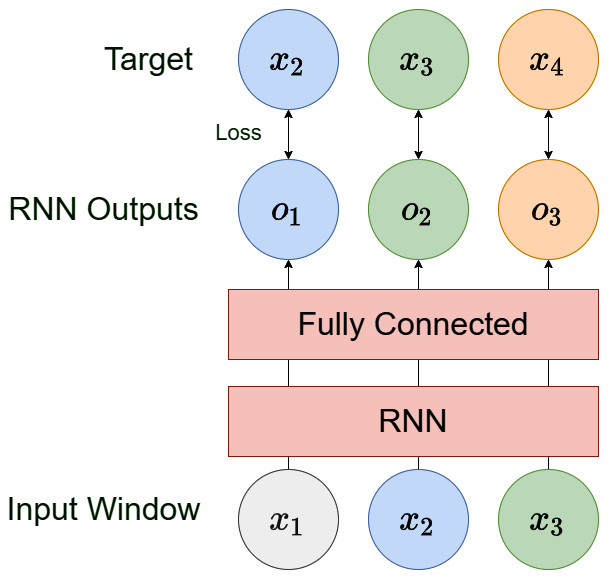
Figure 13.3 – A single-step RNN
Suppose we are using the same example we saw in the dataloader—a time series with the following entries :, ![]() and a window of three. So, one of the samples the dataloader gives will have
and a window of three. So, one of the samples the dataloader gives will have ![]() as the input (x) and
as the input (x) and ![]() as the target. One way we can use this is by passing the sequence through the RNN, ignoring all the outputs except the last one, and using that to predict the target,
as the target. One way we can use this is by passing the sequence through the RNN, ignoring all the outputs except the last one, and using that to predict the target, ![]() . But that is not an efficient use of the samples we have, right? We also know that the output from the first timestep (using
. But that is not an efficient use of the samples we have, right? We also know that the output from the first timestep (using ![]() ) should output
) should output ![]() , the second timestep should output
, the second timestep should output ![]() , and so on. Therefore, we can formulate the RNN in such a way that we maximize the usage of the data and, while training, use these additional points in time to also give a better signal to our model. Now, let’s break down the forward method.
, and so on. Therefore, we can formulate the RNN in such a way that we maximize the usage of the data and, while training, use these additional points in time to also give a better signal to our model. Now, let’s break down the forward method.
forward takes in a single argument called batch, which is a tuple of input and output. So, we unpack batch into two variables, x and y, like so:
x, y = batch
x will have the shape à (batch size, window length, features) and y will have the shape à (batch size, target length, features).
Now we need to pass the input sequence (x) through the RNN (RNN, LSTM, or GRU), like so:
x, _ = self.rnn(x)
As we saw in Chapter 12, Building Blocks of Deep Learning for Time Series, the PyTorch RNNs process the input and return two outputs—hidden states for each timestep and output (which is the hidden state of the last timestep). Here, we need the hidden states from all the timesteps, and therefore we capture that in the x variable. x will now have the dimension à (batch size, window length, hidden size of RNN).
We have the hidden states, but to get the output, we need to apply a fully connected layer over the hidden states, and this fully connected layer should be shared across timesteps. An easy way to do this is to just define a fully connected layer with an input size equal to the hidden size of the RNN and then do the following:
x = self.fc(x)
x is a three-dimensional tensor, and when we use a fully connected layer on a three-dimensional tensor, PyTorch automatically applies the fully connected layer to each of the timesteps. Now, this final output is captured in x, and its dimensions would be a (batch size, window length, 1).
Now, we have got the output of the network, but we also must do a bit of rearrangement to prepare the targets. Currently, y has just the one timestep beyond the window, but if we skip the first timestep from x and concatenate it with y, we would get the target, as we have in Figure 13.3:
y = torch.cat([x[:, 1:, :], y], dim=1)
By using array indexing, we select everything except the first timestep from x and concatenate it with y on the first dimension (which is the window length).
And with that, we have the x and y variables, which we can return, and the BaseModel class will calculate loss and handle the rest of the training. For the entire class, along with the forward method, you can refer to src/dl/models.py.
Let’s test the model we have initialized by passing the batch from the dataloader:
y_hat, y = model(batch)
print("Shape of y_hat: ",y_hat.shape) #-> ([32, 48, 1])
print("Shape of y: ",y.shape) #-> ([32, 48, 1])
Now that the model is working as expected, without errors, let’s start training the model. For that, we can leverage Trainer from PyTorch Lightning. There are so many options in the Trainer class, and a full list of all parameters to tweak the training can be found here: https://pytorch-lightning.readthedocs.io/en/stable/api/pytorch_lightning.trainer.trainer.Trainer.html#pytorch_lightning.trainer.trainer.Trainer.
But here, we are just going to use the bare minimum. Let’s go over the parameters we will be using here one by one:
- auto_select_gpus and gpus—Together, these parameters let us select GPUs for training if present. If we set auto_select_gpus to True and gpus to -1, the Trainer class will choose all GPUs present in the machine, and if there are no GPUs, it falls back to CPU-based training.
- callbacks—PyTorch Lightning has a lot of useful callbacks that can be used during training such as EarlyStopping, ModelCheckpoint, and so on. Most useful callbacks are automatically added even if we don’t explicitly set them, but EarlyStopping is one useful callback that needs to be set explicitly. EarlyStopping is a callback that lets us monitor the validation loss or metrics while training and stop the training when this starts to become worse. This is a form of regularization and helps us keep our model from overfitting to the train data. EarlyStopping has the following major parameters (a full list of parameters can be found here: https://pytorch-lightning.readthedocs.io/en/stable/api/pytorch_lightning.callbacks.EarlyStopping.html):
- monitor—This parameter takes a string input that specifies the exact name of the metric that we want to monitor for early stopping.
- patience—This specifies the number of epochs with no improvement in the monitored metric before the callback stops the training. For instance, if we set patience as 10, the callback will wait for 10 epochs of the degrading metric before stopping the training. There are finer points on these, which are explained in the documentation.
- mode—This is a string input and takes one of min or max. This sets the direction of improvement. In min mode, training will stop when the quantity monitored has stopped decreasing, and in max mode, it will stop when the quantity monitored has stopped increasing.
- min_epochs and max_epochs—These parameters help us set min and max limits to the number of epochs the training should run. If we are using EarlyStopping, min_epochs decides the minimum number of epochs that will be run regardless of the validation loss/metrics, and max_epochs sets the upper limit on the number of epochs. So, even if the validation loss is still decreasing when we reach max_epochs, training will stop.
Glossary
Here are a few terms you should know to fully digest NN training:
Training step—This denotes a single gradient update to the parameter. In batched stochastic gradient descent (SGD), the gradient update after each batch is considered a step.
Batch—A batch is the number of data samples we run through the model and average the gradients over for the update in a training step.
Epoch—An epoch is when the model has seen all the samples in a dataset, or all the batches in the dataset have been used for a gradient update.
So, let’s initialize a bare-bones Trainer class:
trainer = pl.Trainer(
    auto_select_gpus=True,
    gpus=-1,
    min_epochs=5,
    max_epochs=100,
    callbacks=[pl.callbacks.EarlyStopping(monitor="valid_loss", patience=3)],
)
Now, all that is left is to trigger the training by passing in the model and datamodule to a method called fit:
trainer.fit(model, datamodule)
It will run for a while and, depending on when the validation loss starts to increase, it will stop the training. Once the model is trained, we can still use the Trainer class to predict on new data. The prediction uses the predict_step method that we defined in the BaseModel class, which in turn uses the predict method that we defined in the SingleStepRNN model. It’s a very simple method that calls the forward method, takes in the model outputs, and just picks the last timestep from the output (which is the true output that we are projecting into the future). You can see an illustration of this here:
def predict(self, batch):
        y_hat, _ = self.forward(batch)
        return y_hat[:, -1, :]
So, let’s see how we can use the Trainer class to predict on new data (or new dataloaders, to be exact):
pred = trainer.predict(model, datamodule.test_dataloader())
We just need to provide the trained model and the dataloader (here, we use the test dataloader that we have already set up and defined).
Now the output, pred, is a list of tensors, one for each batch in the dataloader. We just need to concatenate them, squeeze out any redundant dimensions, detach them from the computational graph, and convert them to a NumPy array. Here’s how we can do this:
pred = torch.cat(pred).squeeze().detach().numpy()
Now, pred is a NumPy array of predictions for all the items in the test dataframe (which was used to define test_dataloader, but remember we had applied a transformation to the raw time series to standardize it. Now, we need to reverse the transformation. The mean and standard deviation we used for the initial transformation are still stored in the train dataset. We merely retrieve them and inverse the transformation we did earlier, like so:
pred = pred * datamodule.train.std + datamodule.train.mean
Now, we can do all kinds of actions on them, such as evaluate against actuals, visualize the predictions, and so on. Let’s see how well the model has done. To get context, we have included the single-step ML models we did back in Chapter 8, Forecasting Time Series with Machine Learning Models, as well:
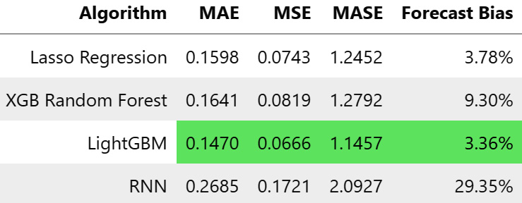
Figure 13.4 – Metrics of the vanilla single-step-ahead RNN on MAC000193 household
It looks like the RNN model did pretty badly. Let’s also look at the predictions visually:
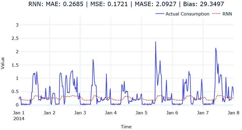
Figure 13.5 – Single-step-ahead RNN predictions for MAC000193 household
We can see that the model has failed to learn the scale of the peaks and the nuances of the patterns. Maybe this is because of the problem that we discussed in terms of RNNs because the seasonality pattern here is spread over 48 timesteps; remember that the pattern requires the RNN to have long-term memory. Let’s quickly swap out the model with LSTM and GRU and see how they are doing. The only thing we need to change is the rnn_type parameter in SingleStepRNNConfig. The notebook has the code to train LSTM and GRU as well. But let’s look at the metrics with LSTM and GRU:
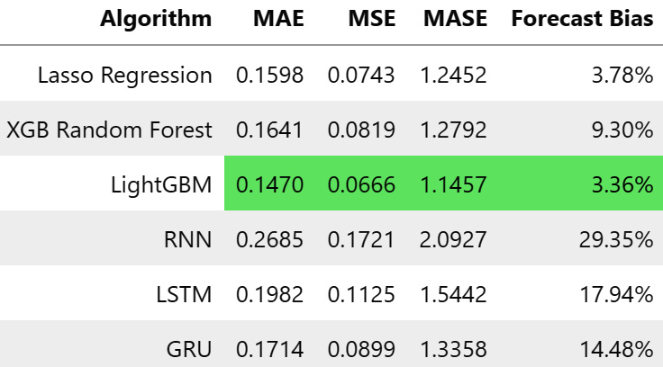
Figure 13.6 – Metrics for single-step-ahead LSTM and GRU on MAC000193 household
Now, it looks competitive. LightGBM is still the best model, but now the LSTM and GRU models are competitive and not entirely lacking, like the vanilla RNN model. If we look at the predictions, we can see that the LSTM and GRU models have managed to capture the pattern much better as well:
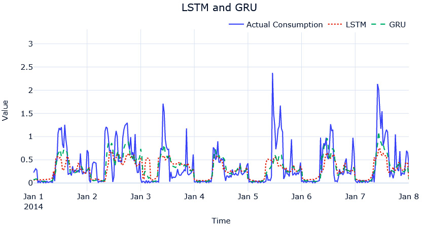
Figure 13.7 – Single-step-ahead LSTM and GRU predictions for MAC000193 household
Things to try
Try changing the parameters of the models and see how it works. How does a bidirectional LSTM perform? Can increasing the window increase performance?
Now that we have seen how a standard RNN can be used for single-step-ahead predictions, let’s look at another modeling pattern that is more flexible than the one we just saw.
Sequence-to-sequence (Seq2Seq) models
We talked in detail about the sequence-to-sequence (Seq2Seq) architecture and the encoder-decoder paradigm in Chapter 12, Building Blocks of Deep Learning for Time Series. Just to refresh your memory, the Seq2Seq model is a kind of an encoder-decoder model by which an encoder encodes the sequence into a latent representation, and then the decoder steps in to carry out the task at hand using this latent representation. This setup is inherently more flexible because of the separation between the encoder (which does the representation learning) and the decoder, which uses the representation for predictions. One of the biggest advantages of this approach, from a time series forecasting perspective, is that the restriction of single step ahead is taken out. Under this modeling pattern, we can extend the forecast to any forecast horizon we want.
In this section, let’s put together a few encoder-decoder models and test out our single-step-ahead forecasts, just like we have been doing with the single-step-ahead RNNs.
Notebook alert
To follow along with the complete code, use the notebook named 03-Seq2Seq RNN.ipynb in the Chapter13 folder and the code in the src folder.
We can use the same mechanism we developed in the last section such as TimeSeriesDataModule, the BaseModel class, and the corresponding code for our Seq2Seq modeling pattern as well. Let’s define a new PyTorch model called Seq2SeqModel, inheriting the BaseModel class. While we are at it, let’s also define a new config file, called Seq2SeqConfig, to set the hyperparameters of the model. The final version of both can be found in src/dl/models.py.
Before we explain the different parameters in the model and the config, let’s talk about the different ways we can set this Seq2Seq model.
RNN-to-fully connected network
For our convenience, let’s restrict the encoder to be from the RNN family—it can be a vanilla RNN, LSTM, or GRU. Now, we saw in Chapter 12, Building Blocks of Deep Learning for Time Series, that in PyTorch, all the models in the RNN family have two outputs—output and hidden states, and we also saw that output is nothing but all the hidden states (final hidden states in stacked RNNs) at all timesteps. The hidden state that we get has the latest hidden states (and cell states, in the case of LSTM) of all layers in the stacked RNN setup. The encoder can be initialized just like we initialized the RNN family of models in the previous section, like so:
self.encoder = nn.LSTM(
                **encoder_params,
                batch_first=True,
            )
And in the forward method, we can just do the following to encode the time series:
o, h = self.encoder(x)
Now, there are a few different ways we can decode the information. The first one we will discuss is using a fully connected layer. Either the fully connected layer can take the latest hidden state from the encoder and predict the desired output or we can flatten all the hidden states into a long vector and use that to predict the output. The latter provides more information to the decoder, but there can be more noise as well. Both are shown in Figure 13.8, using the same example we have been using in the last section as well:
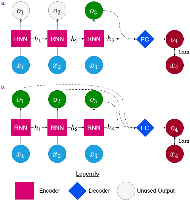
Figure 13.8 – RNN as the encoder and a fully connected layer as the decoder
Let’s also see how we can put together this in code. The decoder in the first case, where we are using just the last hidden state of the encoder, will look like this:
self.decoder = nn.Linear(
                    hidden_size*bi_directional_multiplier, horizon
                )
Here, bi_directional_multiplier is 2 if the encoder was bidirectional and 1 otherwise. This is done because if the encoder is bidirectional, there will be two hidden states concatenated together for each timestep. horizon is the number of timesteps ahead we want to forecast.
In the second case, where we are using the hidden states from all the timesteps, we need to make the decoder, as follows:
self.decoder = nn.Linear(
                    hidden_size * bi_directional_multiplier * window_size, horizon
                )
Here, the input vector will be the flattened vector of all the hidden states from all the timesteps, and hence the input dimension would be hidden_size * window_size.
And in the forward method, we can do the following for case 1:
y_hat = self.decoder(o[:,-1,:]).unsqueeze(-1)
Here, we are just taking the hidden state from the latest timestep and unsqueezing to maintain three dimensions as the target, y.
For case 2, we can do the following:
y_hat = self.decoder(o.reshape(o.size(0), -1)).unsqueeze(-1)
Here, we first reshape the entire hidden state to flatten it and then pass it through the decoder to get the predictions. We unsqueeze to insert the dimension we collapsed so that the output and target, y, have the same dimensions.
Even though, in theory, we can use the fully connected decoder to predict as much into the future as possible, practically, there are limitations. When we have a large number of steps to forecast, the model will have to learn that big of a matrix to generate those outputs, and that becomes harder as the matrix becomes bigger. Another point worth noting is that each of these predictions happens independently with the information encoded in the latent representation. For instance, the prediction of five timesteps ahead is only dependent on the latent representation from the encoder and not predictions of timesteps 1 to 4. Let’s look at another type of Seq2Seq, which makes the decoding more flexible and aware of the temporal aspect of the problem.
RNN-to-RNN
Instead of using a fully connected layer as the decoder, we can use another RNN for decoding as well—so, one model from the RNN family takes care of the encoding and another model from the RNN family takes care of the decoding. Initializing the decoder in the model is also similar to initializing the encoder. If we want an LSTM model as the decoder, we can do the following:
self.decoder = nn.LSTM(
                **decoder_params,
                batch_first=True,
            )
Let’s develop our understanding of how this is done through a visual representation:
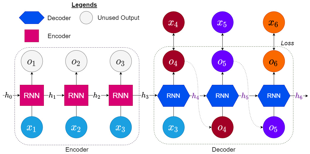
Figure 13.9 – RNN as the encoder and decoder
The encoder part remains the same: it takes in the input window ![]() to
to ![]() and produces outputs,
and produces outputs, ![]() to
to ![]() , and the last hidden state,
, and the last hidden state, ![]() . Now, we have another decoder (a model from the RNN family) that takes in
. Now, we have another decoder (a model from the RNN family) that takes in ![]() , as the initial hidden state, and the latest input from the window to produce the next output. And now, this output is fed back into the RNN as the input and we produce the next output, and this cycle continues until we have got the required number of timesteps in our prediction.
, as the initial hidden state, and the latest input from the window to produce the next output. And now, this output is fed back into the RNN as the input and we produce the next output, and this cycle continues until we have got the required number of timesteps in our prediction.
Some of you may be wondering why we don’t use the target window (![]() to
to ![]() ) during decoding as well. In fact, this is a valid way of training the model and is called teacher forcing in the literature. This has strong connections to maximum likelihood and is explained well in the Deep Learning book by Goodfellow et al. (see the Further reading section). So, instead of feeding in the output of the model from the previous timestep as the input to the RNN at the current timestep, we feed in the real observation, thereby eliminating the error that might have crept in in the previous timestep.
) during decoding as well. In fact, this is a valid way of training the model and is called teacher forcing in the literature. This has strong connections to maximum likelihood and is explained well in the Deep Learning book by Goodfellow et al. (see the Further reading section). So, instead of feeding in the output of the model from the previous timestep as the input to the RNN at the current timestep, we feed in the real observation, thereby eliminating the error that might have crept in in the previous timestep.
While this sounds like the most straightforward thing to do, it does come with a few disadvantages as well. The main one is that the kinds of inputs that the decoder sees during training may not the same as the ones it will see during actual prediction. During prediction, we will still be feeding the output of the model in the previous step to the decoder. This is because in the inference mode, we do not have access to real observations in the future. This can cause problems in some cases. One way to mitigate this problem is to randomly choose between the model’s output at the previous timestep and real observation while training (Bengio et al., 2015).
Reference check
The research paper by Bengio et al., which proposed teacher forcing, is cited in the References section.
Now, let’s see how we can code the forward method for both these cases using a parameter called teacher_forcing_ratio, which is a decimal from 0 to 1. This decides how frequently teacher forcing is implemented. For instance, if teacher_forcing_ratio = 0, then teacher forcing is never done, and if teacher_forcing_ratio = 1, then teacher forcing is always done.
The following code block has all the code necessary for decoding, and it comes with line numbers so that we can go line by line and explain what we are doing:
01  y_hat = torch.zeros_like(y, device=y.device)
02  dec_input = x[:, -1:, :]
03  for i in range(y.size(1)):
04      out, h = self.decoder(dec_input, h)
05      out = self.fc(out)
06      y_hat[:, i, :] = out.squeeze(1)
07      #decide if we are going to use teacher forcing or not
08      teacher_force = random.random() < teacher_forcing_ratio
09      if teacher_force:
10          dec_input = y[:, i, :].unsqueeze(1)
11      else:
12          dec_input = out
The first thing we need to do is declare a placeholder to store the desired output during decoding. In line number 1, we do that by using zeros_like, which generates a tensor with all zeros with the same dimension as y, and in line number 2, we set the initial input to the decoder as the last timestep in the input window. Now, we are all set to start the decoding process, and for that, in line number 3, we start a loop to run y.size(1) times. If you remember the dimensions of y, the second dimension was the sequence length, so we need to run the decoding process that many times.
In line number 4, we pass in the last input from the input window and the hidden state from the encoder to the decoder, and it returns the current output and the hidden state. We capture the current hidden state in the same variable, overwriting the old one. If you remember, the output from the RNN is the hidden state, and we will need to pass it through a fully connected layer for the prediction. So, in line number 5, we do just that. In line number 6, we store the output from the fully connected layer to the i-th timestep in y_hat.
Now, we just have one more thing to do—decide whether to use teacher forcing or not and move on to decoding the next timestep. This we can do by generating a random number between 0 and 1 and checking whether that number is less than the teacher_forcing_ratio parameter or not. random.random() samples a number from a uniform distribution between 0 and 1. If the teacher_forcing_ratio parameter is 0.5, checking whether random.random()<teacher_forcing_ratio automatically ensures we only do teacher forcing 50% of the time. So, in line number 8, we do this check and get a Boolean output, teacher_force, which tells us whether we need to do teacher forcing in the next timestep or not. For teacher forcing, we store the current timestep from y as dec_input (line number 10). Otherwise, we store the current output as dec_input (line number 12), and this dec_input parameter is used as the input to the RNN in the next timestep.
Now, all of this (both the fully connected decoder and the RNN decoder) has been put together into a single class called Seq2SeqModel in src/dl/models.py, and a config class (Seq2SeqConfig) has also been defined that has all the options and hyperparameters of the models. Let’s take a look at the different parameters in the config:
- encoder_type—A string parameter that takes in one of three values: RNN, LSTM, or GRU. This decides the sequence model we need to use as the encoder.
- decoder_type—A string parameter that takes in one of four values: RNN, LSTM, GRU, or FC (for fully connected). This decides the sequence model we need to use as the decoder.
- encoder_params and decoder_params—These parameters take a dictionary of key-value pairs as the input. These are the hyperparameters of the encoder and the decoder, respectively. For the RNN family of models, there is another config class, RNNConfig, which sets standard hyperparameters such as hidden_size, num_layers, and so on. And for the FC decoder, we need to give two parameters: window_size as the number of timesteps included in the input window, and horizon as the number of timesteps ahead we want to be forecasting.
- decoder_use_all_hidden—We discussed two ways we can use the fully connected decoder. This parameter is a flag that switches between the two. If True, the fully connected decoder will flatten the hidden states of all timesteps and use them for the prediction, and if False, it will just use the last hidden state.
- teacher_forcing_ratio—We discussed teacher forcing earlier, and this parameter decided the strength of teacher forcing while training. If 0, there will be no teacher forcing, and if 1, every timestep will be teacher-forced.
- optimizer_params, lr_scheduler, lr_scheduler_params—These are parameters that let us tweak the optimization procedure. Let’s not worry about these for now because all of them have been set to intelligent defaults.
Now, with this config and the model, let’s run a few experiments. These work exactly the same as the set of experiments we ran in the previous section. The exact code for the experiments is available in the accompanying notebook. So, we ran the following experiments:
- LSTM_FC_last_hidden—Encoder = LSTM/Decoder = Fully Connected, using just the last hidden state
- LSTM_FC_all_hidden—Encoder = LSTM/Decoder = Fully Connected, using all the hidden states
- LSTM_LSTM—Encoder = LSTM/Decoder = LSTM
Let’s see how they performed on the metrics we have been tracking:
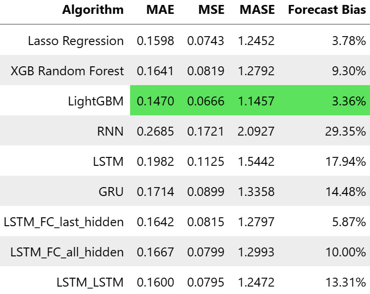
Figure 13.10 – Metrics for Seq2Seq models on MAC000193 household
The Seq2Seq models seem to be performing better on the metrics and the LSTM_LSTM model is even better than the Random Forest model.
There are visualizations of each of these forecasts in the notebook. I urge you to look at those visualizations, zoom in, look at different places in the horizon, and so on. The astute observers among you must have figured out something weird with the forecast. Let’s look at a zoomed-in version (on 1 day) of the forecasts we generated to make that point clear:
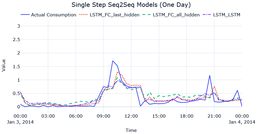
Figure 13.11 – Single-step-ahead Seq2Seq predictions for MAC000193 household (1 day)
What do you see now? Focus on the peaks in the time series. Are they aligned or do they seem at an offset? This phenomenon that you are seeing now is when a model learns to mimic the last seen timestep (like the naïve forecast) rather than learn the true pattern in the data. We will be getting good metrics and we might be happy with the forecast, but upon investigation, we can see that this is not the forecast we want. This is especially true in the case of single-step-ahead models where we are just optimizing to predict the next timestep. Therefore, the model has no real incentive to learn long-term patterns, such as seasonality and so on, and ends up learning a model like the naïve forecast.
Models that are trained to predict longer horizons overcome this problem because, in this scenario, the model is forced to learn the longer-term patterns in the model. Although multi-step forecasting is a topic that will be covered in detail in Chapter 17, Multi-Step Forecasting, let’s do a little bit of a sneak peek now. In the notebook, we also train multi-step models using the Seq2Seq models.
The only changes we need to make are these:
- The horizon we define in the datamodule and the models should change.
- The way we evaluate the models should also have a small change.
Let’s see how we can define a datamodule for multi-step forecasting. We have chosen to forecast a complete day, which is 48 timesteps. And as an input window, we are giving ![]() timesteps:
timesteps:
HORIZON = 48
WINDOW = 48*2
datamodule = TimeSeriesDataModule(data = sample_df[[target]],
        n_val = sample_val_df.shape[0],
        n_test = sample_test_df.shape[0],
        window = WINDOW,
        horizon = HORIZON,
        normalize = "global", # normalizing the data
        batch_size = 32,
        num_workers = 0)
Now that we have the datamodule, we can initialize the models just like before and train them. The only change we have to make now is while predicting.
In the single-step setting, at each timestep, we were predicting the next one. But now, we are predicting the next 48 timesteps, at each step. There are multiple ways to look at this and measure the metrics, which we will cover in detail in Part 3. For now, let’s choose a heuristic and say that we are considering that we are running this model only once a day, and each such prediction has 48 timesteps. But the test dataloader still increments by one—in other words, the test dataloader still gives us the next 48 timesteps, for each timestep. So, executing the following code, we will get a prediction array with dimensions—(timesteps, horizon):
pred = trainer.predict(model, datamodule.test_dataloader())
# pred is a list of outputs, one for each batch
pred = torch.cat(pred).squeeze().detach().numpy()
The predictions start at 2014, Jan 1 00:00:00. So, if we select the 48 timesteps, every 48 timesteps apart, it’ll be like considering only predictions that are made at the beginning of the day. Using a bit of fancy indexing numpy provides us, it is easy to do just that:
pred = pred[0::48].ravel()
We start at index 0, which is the first prediction of 48 timesteps, and pick every 48 indices (which are timesteps) and just flatten the array. We will get an array of predictions with the desired shape, and then the standard procedure of inverse transformation and metric calculation, and so on, proceeds.
The notebook has the code to do the following experiments:
- MultiStep LSTM_FC_last_hidden—Encoder = LSTM/Decoder = Fully Connected Layer, using only the last hidden state
- MultiStep LSTM_FC_all_hidden—Encoder = LSTM/Decoder = Fully Connected Layer, using all the hidden states
- MultiStep LSTM_LSTM_teacher_forcing_0.0—Encoder = LSTM/ Decoder = LSTM, using no teacher forcing
- MultiStep LSTM_LSTM_teacher_forcing_0.5—Encoder = LSTM/ Decoder = LSTM, using stochastic teacher forcing (randomly, 50% of the time teacher forcing is enabled)
- MultiStep LSTM_LSTM_teacher_forcing_1.0—Encoder = LSTM/ Decoder = LSTM, using complete teacher forcing
Let’s look at the metrics of these experiments:
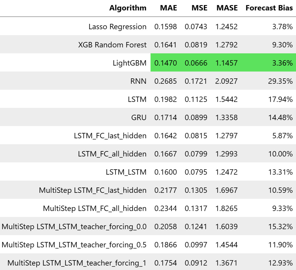
Figure 13.12 – Metrics for multi-step Seq2Seq models on MAC000193 household
Although we cannot compare single-step-ahead accuracy to multi-step ones, for the time being, let’s suspend that concern and use the single-step metrics as in the best-case scenario. So, we can see that our model that predicts 1 day ahead (48 timesteps) is not such a bad model after all, and if we visualize the predictions, the problem of imitating naïve forecasts is also not present because now the model is forced to learn long-term models and forecasts:
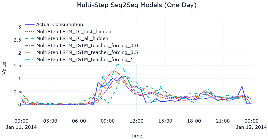
Figure 13.13 – Multi-step-ahead Seq2Seq predictions for MAC000193 household (1 day)
We can see that the model has tried to learn the daily patterns because it is forced to predict the next 48 timesteps. With some tuning and other training tricks, we might get a better model as well. But running a separate model for all LCLid (consumer ID) instances in the dataset may not be the best option, both from an engineering and a modeling perspective. We will tackle strategies for global modeling in Chapter 15, Strategies for Global Deep Learning Forecasting Models.
Things to try
Can you train a better model? Tweak the hyperparameters and try to get better performance. Use GRUs or combine a GRU with an LSTM—the possibilities are endless.
Congratulations on getting through yet another hands-on and practical chapter. If this is the first time you are training NNs, I hope this lesson has made you confident enough to try more: trying and experimenting with these techniques is the best way to learn.
Summary
Although we learned about the basic blocks of DL in the previous chapter, we put all of that into action while we used those blocks in common modeling patterns using PyTorch.
We saw how standard sequence models such as RNN, LSTM, and GRU can be used for time series prediction, and then we moved on to another paradigm of models, called Seq2Seq models. Here, we talked about how we can mix and match encoders and decoders to get the model we want. Encoders and decoders can be arbitrarily complex. Although we looked at simple encoders and decoders, it is very much possible to have something like a combination of a convolution block and an LSTM block working together for the encoder. Last but not least, we talked about teacher forcing and how it can help models train and converge faster and also with some performance boost.
In the next chapter, we will be tackling a subject that has captured a lot of attention (pun intended) in the past few years: attention and transformers.
Reference
Samy Bengio, Oriol Vinyals, Navdeep Jaitly, and Noam Shazeer (2015). Scheduled Sampling for Sequence Prediction with Recurrent Neural Networks. Proceedings of the 28th International Conference on Neural Information Processing Systems - Volume 1 (NIPS’15): https://proceedings.neurips.cc/paper/2015/file/e995f98d56967d946471af29d7bf99f1-Paper.pdf.
Further reading
You can check out the following sources for further reading:
- From PyTorch to PyTorch Lightning by Alfredo Canziani and William Falcon: https://www.youtube.com/watch?v=DbESHcCoWbM
- Deep Learning—Ian Goodfellow, Yoshua Bengio, and Aaron Courville (pages 376-377): https://www.deeplearningbook.org/contents/rnn.html
- A Short Chronology Of Deep Learning For Tabular Data by Sebastian Raschka: https://sebastianraschka.com/blog/2022/deep-learning-for-tabular-data.html