
Chapter 6 Beyond elasticity: Plasticity, yielding and ductility
- 6.1 Introduction and synopsis 112
- 6.2 Strength, plastic work and ductility: definition and measurement 112
- 6.3 The big picture: charts for yield strength 116
- 6.4 Drilling down: the origins of strength and ductility 119
- 6.5 Manipulating strength 127
- 6.6 Summary and conclusions 136
- 6.7 Further reading 136
- 6.8 Exercises 137
- 6.9 Exploring design with CES 138
- 6.10 Exploring the science with CES Elements 138
The verb ‘to yield’ has two seemingly contradictory meanings. To yield under force is to submit to it, to surrender. To yield a profit has a different, more comfortable connotation: to bear fruit, to be useful. The yield strength, when speaking of a material, is the stress beyond which it becomes plastic. The term is well chosen: yield and the plasticity that follows can be profitable—it allows metals to be shaped and it allows structures to tolerate impact and absorb energy. But the unplanned yield of the span of a bridge or of the wing spar of an aircraft or of the forks of your bicycle spells disaster.
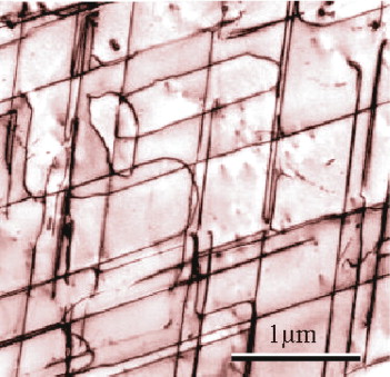
Dislocations in the intermetallic compound, Ni3Al. (Image courtesy of C. Rentenberger and H. P. Karnthaler, Institute of Materials Physics, University of Vienna, Austria)
6.1 Introduction and synopsis
The verb ‘to yield’ has two seemingly contradictory meanings. To yield under force is to submit to it, to surrender. To yield a profit has a different, more comfortable connotation: to bear fruit, to be useful. The yield strength, when speaking of a material, is the stress beyond which it becomes plastic. The term is well chosen: yield and the plasticity that follows can be profitable—it allows metals to be shaped and it allows structures to tolerate impact and absorb energy. But the unplanned yield of the span of a bridge or of the wing spar of an aircraft or of the forks of your bicycle spells disaster.
This chapter is about yield and plasticity. For that reason it is mainly (but not wholly) about metals: it is the plasticity of iron and steel that made them the structural materials on which the Industrial Revolution was built, enabling the engineering achievements of the likes of Telford1 and Brunel2. The dominance of metals in engineering, even today, derives from their ability to be rolled, forged, drawn and stamped.
6.2 Strength, plastic work and ductility: definition and measurement
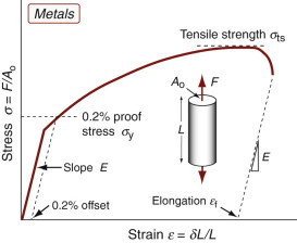
Yield properties and ductility are measured using the standard tensile tests introduced in Chapter 4, with the materials taken to failure. Figures 6.1–6.3 show the types of stress–strain behavior observed in different material classes. The yield strength σy (or elastic limit σel)—units: MPa or MN/m2—requires careful definition. For metals, the onset of plasticity is not always distinct so we identify σy with the 0.2% proof stress—that is, the stress at which the stress–strain curve for axial loading deviates by a strain of 0.2% from the linear elastic line as shown in Figure 6.1. It is the same in tension and compression. When strained beyond the yield point, most metals work harden, causing the rising part of the curve, until a maximum, the tensile strength, is reached. This is followed in tension by nonuniform deformation (necking) and fracture.
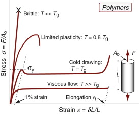
For polymers, σy is identified as the stress at which the stress–strain curve becomes markedly nonlinear: typically, a strain of 1% (Figure 6.2). The behavior beyond yield depends on the temperature relative to the glass temperature Tg. Well below Tg most polymers are brittle. As Tg is approached, plasticity becomes possible until, at about Tg, thermoplastics exhibit cold drawing: large plastic extension at almost constant stress during which the molecules are pulled into alignment with the direction of straining, followed by hardening and fracture when alignment is complete. At still higher temperatures, thermoplastics become viscous and can be moulded; thermosets become rubbery and finally decompose.
The yield strength σy of a polymer–matrix composite is best defined by a set deviation from linear elastic behavior, typically 0.5%. Composites that contain fibres (and this includes natural composites like wood) are a little weaker (up to 30%) in compression than tension because the fibres buckle on a small scale.
Plastic strain, εpl, is the permanent strain resulting from plasticity; thus it is the total strain εtot minus the recoverable, elastic, part:
The ductility is a measure of how much plastic strain a material can tolerate. It is measured in standard tensile tests by the elongation εf (the tensile strain at break) expressed as a percentage (Figures 6.1 and 6.2). Strictly speaking, εf is not a material property because it depends on the sample dimensions—the values that are listed in handbooks and in the CES software are for a standard test geometry—but it remains useful as an indicator of the ability of a material to be deformed.
In Chapter 4, the area under the elastic part of the stress–strain curve was identified as the elastic energy stored per unit volume (![]() ). Beyond the elastic limit plastic work is done in deforming a material permanently by yield or crushing. The increment of plastic work done for a small permanent extension or compression dL under a force F, per unit volume V = ALo, is
). Beyond the elastic limit plastic work is done in deforming a material permanently by yield or crushing. The increment of plastic work done for a small permanent extension or compression dL under a force F, per unit volume V = ALo, is
Thus, the plastic work per unit volume at fracture, important in energy-absorbing applications, is
which is just the area under the stress–strain curve.
Example 6.1
A metal rod with a yield strength σy = 500 MPa and a density ρ = 8000 kg/m3 is uniformly stretched to a strain of 0.1 (10%). How much plastic work is absorbed per unit volume by the rod in this process? Assume that the material is elastic perfectly-plastic, that is it deforms plastically at a constant stress σy. Compare this plastic work with the elastic energy calculated in Example 4.3.
Answer. Assuming that the material is ‘elastic perfectly-plastic’, that is, the stress equals the yield strength up to failure, the plastic energy per unit volume at failure is:
This plastic energy is 80 times the elastic strain energy of 625 kJ/m3 in Example 4.3, but is still only 0.015% of the chemical energy stored in the same mass of gasoline.
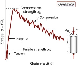
Ceramics and glasses are brittle at room temperature (Figure 6.3). They do have yield strengths, but these are so enormously high that, in tension, they are never reached: the materials fracture first. Even in compression ceramics and glasses crush before they yield. To measure their yield strengths, special tests that suppress fracture are needed. It is useful to have a practical measure of the strength of ceramics to allow their comparison with other materials. That used here is the compressive crushing strength, and since it is not true yield even though it is the end of the elastic part of the stress–strain curve, we call it the elastic limit and give it the symbol σel.
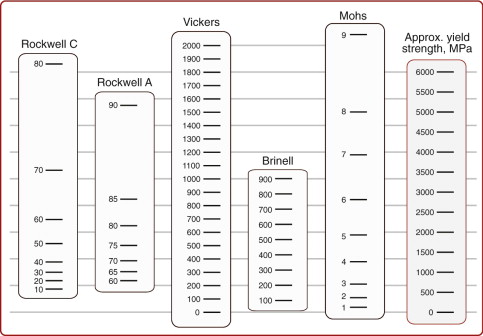
Tensile and compression tests are not always convenient: you need a large sample and the test destroys it. The hardness test (Figure 6.4) avoids these problems, although it has problems of its own. In it, a pyramidal diamond or a hardened steel ball is pressed into the surface of the material, leaving a tiny permanent indent, the size of which is measured with a microscope. The indent means that plasticity has occurred, and the resistance to it—a measure of strength—is the load F divided by the area A of the indent projected onto a plane perpendicular to the load:
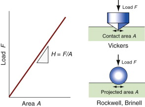
Figure 6.4 The hardness test. The Vickers test uses a diamond pyramid; the Rockwell and Brinell tests use a steel sphere.

The indented region is surrounded by material that has not deformed, and this constrains it so that H is larger than the yield strength σy; in practice it is about 3σy. Strength, as we have seen, is measured in units of MPa, and since H is a strength it would be logical and proper to measure it in MPa too. But things are not always logical and proper, and hardness scales are among those that are not. A commonly used scale, that of Vickers, symbol Hv, uses units of kg/mm2, with the result that

Figure 6.5 shows conversions to other scales.
The hardness test has the advantage of being non-destructive, so strength can be measured without destroying the component, and it requires only a tiny volume of material. But the information it provides is less accurate and less complete than the tensile test, so it is not used to provide critical design data.
6.3 The big picture: charts for yield strength
Strength can be displayed on material property charts. Two are particularly useful: the strength–density chart and the modulus–strength chart.
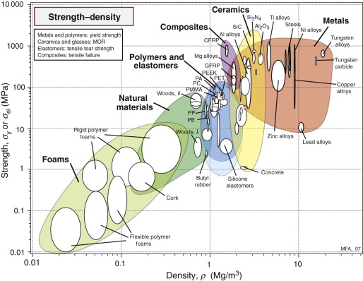
The strength–density chart
Figure 6.6 shows the yield strength σy or elastic limit σel plotted against density ρ. The range of strength for engineering materials, like that of the modulus, spans about six decades: from less than 0.01 MPa for foams, used in packaging and energy-absorbing systems, to 104 MPa for diamond, exploited in diamond tooling for machining and as the indenter of the Vickers hardness test. Members of each family again cluster together and can be enclosed in envelopes, each of which occupies a characteristic part of the chart.
Example 6.2
An unidentified metal from a competitor’s product is measured to have a ‘Rockwell A’ hardness of 50 and a density of approximately 8800 kg/m3. Estimate its Vickers hardness and its yield strength. Locate its position on the strength–density chart (Figure 6.6). What material is it likely to be?
Answer. From Figure 6.5, the Vickers hardness is approximately 510 and the yield strength is approximately 1600 MPa (which agrees reasonably with Equation 6.4). This is a strong metal. It falls near the top of the nickel alloys on the strength–density chart.
Comparison with the modulus–density chart (Figure 4.7) reveals some marked differences. The modulus of a solid is a well-defined quantity with a narrow range of values. The strength is not. The strength range for a given class of metals, such as stainless steels, can span a factor of 10 or more, while the spread in stiffness is at most 10%. Since density varies very little (Chapter 4), the strength bubbles for metals are long and thin. The wide ranges for metals reflect the underlying physics of yielding and present designers with an opportunity for manipulation of the strength by varying composition and process history. Both are discussed later in this chapter.
Polymers cluster together with strengths between 10 and 100 MPa. The composites CFRP and GFRP have strengths that lie between those of polymers and ceramics, as we might expect since they are mixtures of the two. The analysis of the strength of composites is not as straightforward as for modulus in Chapter 4, though the same bounds (with strength replacing modulus) generally give realistic estimates.
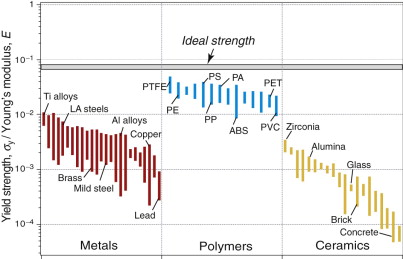
The modulus–strength chart
Figure 6.7 shows Young’s modulus, E, plotted against yield strength, σy or elastic limit σel. This chart allows us to examine a useful material characteristic, the yield strain, σy/E, meaning the strain at which the material ceases to be linearly elastic. On log axes, contours of constant yield strain appear as a family of straight parallel lines, as shown in Figure 6.7. Engineering polymers have large yield strains, between 0.01 and 0.1; the values for metals are at least a factor of 10 smaller. Composites and woods lie on the 0.01 contour, as good as the best metals. Elastomers, because of their exceptionally low moduli, have values of σy/E in the range 1 to 10, much larger than any other class of material.
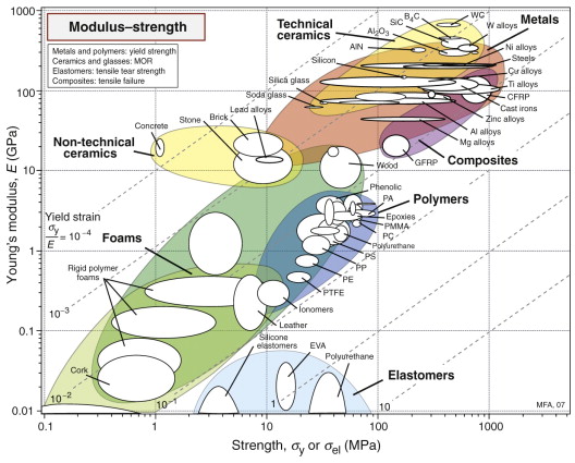
Figure 6.7 The Young’s modulus–strength chart. The contours show the strain at the elastic limit, σy/E.
This chart has many other applications, notably in selecting materials for springs, elastic diaphragms, flexible couplings and snap-fit components. We explore these in Chapter 7.
6.4 Drilling down: the origins of strength and ductility
Perfection: the ideal strength
The bonds between atoms, like any other spring, have a breaking point. Figure 6.8 shows a stress–strain curve for a single bond. Here an atom is assumed to occupy a cube of side ao (as was assumed in Chapter 4) so that a force F corresponds to a stress ![]() . The force stretches the bond from its initial length ao to a new length a, giving a strain (a − ao)/ao. When discussing the modulus in Chapter 4 we focused on the initial, linear part of this curve, with a slope equal to the modulus, E. Stretched farther, the curve passes through a maximum and sinks to zero as the atoms lose communication. The peak is the bond strength—if you pull harder than this it will break. The same is true if you shear it rather than pull it.
. The force stretches the bond from its initial length ao to a new length a, giving a strain (a − ao)/ao. When discussing the modulus in Chapter 4 we focused on the initial, linear part of this curve, with a slope equal to the modulus, E. Stretched farther, the curve passes through a maximum and sinks to zero as the atoms lose communication. The peak is the bond strength—if you pull harder than this it will break. The same is true if you shear it rather than pull it.
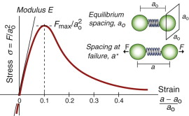
Figure 6.8 The stress–strain curve for a single atomic bond (it is assumed that each atom occupies a cube of side ao).
The distance over which inter-atomic forces act is small—a bond is broken if it is stretched to more than about 10% of its original length. So the force needed to break a bond is roughly:

where S, as before, is the bond stiffness. On this basis the ideal strength of a solid should therefore be roughly
(remembering that E = So/ao, equation (4.17))or
This doesn’t allow for the curvature of the force–distance curve; more refined calculations give a ratio of 1/15.
Figure 6.9 shows σy/E for metals, polymers and ceramics. None achieves the ideal value of 1/10; most don’t even come close. Why not? It’s a familiar story: like most things in life, materials are imperfect.
Crystalline imperfection: defects in metals and ceramics
Crystals contain imperfections of several kinds. Figure 6.10 introduces the broad families, distinguished by their dimensionality. At the top left are point defects. All crystals contain vacancies, shown in (a): sites at which an atom is missing. They play a key role in diffusion, creep and sintering (Chapter 13), but we don’t need them for the rest of this chapter because they do not influence strength. The others do.
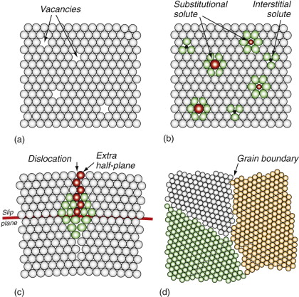
Figure 6.10 Defects in crystals. (a) Vacancies–missing atoms. (b) Foreign (solute) atom on interstitial and substitutional sites. (c) A dislocation—an extra half-plane of atoms. (d) Grain boundaries.
No crystal is totally, 100%, pure and perfect. Some impurities are inherited from the process by which the material was made; more usually they are deliberately added, creating alloys: a material in which a second (or third or fourth) element is dissolved. ‘Dissolved’ sounds like salt in water, but these are solid solutions. Figure 6.10(b) shows both a substitutional solid solution (the dissolved atoms replace those of the host) and an interstitial solid solution (the dissolved atoms squeeze into the spaces or ‘interstices’ between the host atoms). The dissolved atoms or solute rarely has the same size as those of the host material, so it distorts the surrounding lattice. The red atoms here are substitutional solute, some bigger and some smaller than those of the host; the cages of host atoms immediately surrounding them, shown green, are distorted. If the solute atoms are particularly small, they don’t need to replace a host atom; instead, they dissolve interstitially like the black atoms in the figure, again distorting the surrounding lattice. So solute causes local distortion; this distortion is one of the reasons that alloys are stronger than pure materials, as we shall see in a moment.
Now to the key player, portrayed in Figure 6.10(c): the dislocation. ‘Dislocated’ means ‘out of joint’ and this is not a bad description of what is happening here. The upper part of the crystal has one more double-layer of atoms than the lower part (the double-layer is needed to get the top-to-bottom registry right). It is dislocations that make metals soft and ductile. Dislocations distort the lattice—here the green atoms are the most distorted—and because of this they have elastic energy associated with them. If they cost energy, why are they there? To grow a perfect crystal just one cubic centimeter in volume from a liquid or vapour, about 1023 atoms have to find their proper sites on the perfect lattice, and the chance of this happening is just too small. Even with the greatest care in assembling them, all crystals contain point defects, solute atoms and dislocations.
Most contain yet more drastic defects, among them grain boundaries. Figure 6.10(d) shows such boundaries. Here three perfect, but differently oriented, crystals meet; the individual crystals are called grains, the meeting surfaces are grain boundaries. In this sketch the atoms of the three crystals have been given different colours to distinguish them, but here they are the same atoms. In reality grain boundaries form in pure materials (when all the atoms are the same) and in alloys (when the mixture of atoms in one grain may differ in chemical composition from those of the next).
Now put all this together. The seeming perfection of the steel of a precision machine tool or of the polished case of a gold watch is an illusion: they are riddled with defects. Imagine all the frames of Figure 6.10 superimposed and you begin to get the picture. Between them they explain diffusion, strength, ductility, electrical resistance, thermal conductivity and much more.
So defects in crystals are influential. For the rest of this section we focus on getting to know just one of them: the dislocation.
Dislocations and plastic flow
Recall that the strength of a perfect crystal computed from inter-atomic forces gives an ‘ideal strength’ around E/15 (where E is the modulus). In reality the strengths of engineering materials are nothing like this big; often they are barely 1% of it. This was a mystery until halfway through the last century—a mere 60 years ago—when an Englishman, G. I. Taylor3, and a Hungarian, Egon Orowan4, realized that a ‘dislocated’ crystal could deform at stresses far below the ideal. So what is a dislocation, and how does it enable deformation?
Figure 6.11(a) shows how to make a dislocation. The crystal is cut along an atomic plane up to the line shown as ⊥—⊥, the top part is slid across the bottom by one full atom spacing, and the atoms are reattached across the cut plane to give the atom configuration shown in Figure 6.11(b). There is now an extra half-plane of atoms with its lower edge along the ⊥—⊥ line, the dislocation line—the line separating the part of the plane that has slipped from the part that has not. This particular configuration is called an edge dislocation because it is formed by the edge of the extra half-plane, represented by the symbol ⊥.
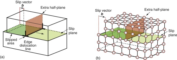
Figure 6.11 (a) Making a dislocation by cutting, slipping and rejoining bonds across a slip plane. (b) The atom configuration at an edge dislocation in a simple cubic crystal. The configurations in other crystal structures are more complex but the principle remains the same.
When a dislocation moves it makes the material above the slip plane slide relative to that below, producing a shear strain. Figure 6.12 shows how this happens. At the top is a perfect crystal. In the central row a dislocation enters from the left, sweeps through the crystal and exits on the right. By the end of the process the upper part has slipped by b, the slip vector (or Burger’s vector) relative to the part below. The result is the shear strain γ shown at the bottom.
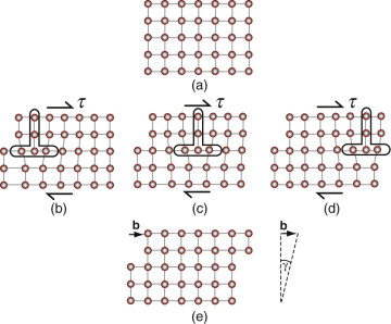
Figure 6.12 An initially perfect crystal is shown in (a). The passage of the dislocation across the slip plan, shown in the sequence (b), (c) and (d), shears the upper part of the crystal over the lower part by the slip vector b. When it leaves the crystal has suffered a shear strain γ.
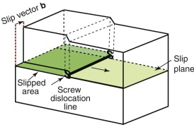
There is another way to make a dislocation in a crystal. After making the cut in Figure 6.11(a), the upper part of the crystal can be displaced parallel to the edge of the cut rather than normal to it, as in Figure 6.13. That too creates a dislocation, but one with a different configuration of atoms along its line—one more like a corkscrew than like a squashed worm—and for this reason it is called a screw dislocation. We don’t need the details of its structure; it is enough to know that its properties are like those of an edge dislocation except that when it sweeps through a crystal (moving normal to its line), the lattice is displaced parallel to the dislocation line, not normal to it. All dislocations are either edge or screw or mixed, meaning that they are made up of little steps of edge and screw. The line of a mixed dislocation can be curved but every part of it has the same slip vector b because the dislocation line is just the boundary of a plane on which a fixed displacement b has occurred.
It is far easier to move a dislocation through a crystal, breaking and remaking bonds only along its line as it moves, than it is to simultaneously break all the bonds in the plane before remaking them. It is like moving a heavy carpet by pushing a fold across it rather than sliding the whole thing at one go. In real crystals it is easier to make and move dislocations on some planes than on others. The preferred planes are called slip planes and the preferred directions of slip in these planes are called slip directions. A slip plane is shown in gray and a slip direction as an arrow on the FCC and BCC unit cells of Figure 4.11.
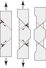
Slip displacements are tiny—one dislocation produces a displacement of about 10−10 m. But if large numbers of dislocations traverse a crystal, moving on many different planes, the shape of a material changes at the macroscopic length scale. Figure 6.14 shows just two dislocations traversing a sample loaded in tension. The slip steps (here very exaggerated) cause the sample to get a bit thinner and longer. Repeating this millions of times on many planes gives the large plastic extensions observed in practice. Since none of this changes the average atomic spacing, the volume remains unchanged.
Why does a shear stress make a dislocation move?
Crystals resist the motion of dislocations with a friction-like resistance f per unit length—we will examine its origins in a moment. For yielding to take place the external stress must overcome the resistance f.
Imagine that one dislocation moves right across a slip plane, traveling the distance L2, as in Figure 6.15. In doing so, it shifts the upper half of the crystal by a distance b relative to the lower half. The shear stress τ acts on an area L1L2, giving a shear force Fs = τL1L2 on the surface of the block. If the displacement parallel to the block is b, the force does work
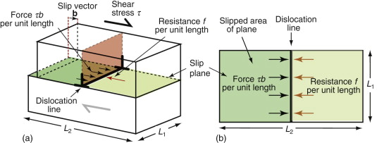
This work is done against the resistance f per unit length, or f L1 on the length L1, and it does so over a displacement L2 (because the dislocation line moves this far against f), giving a total work against f of fL1L2. Equating this to the work W done by the applied stress τ gives
This result holds for any dislocation—edge, screw or mixed. So, provided the shear stress τ exceeds the value f/b it will make dislocations move and cause the crystal to shear.
Line tension
The atoms near the core of a dislocation are displaced from their proper positions, as shown by green atoms back in Figure 6.10(c), and thus they have higher potential energy. To keep the potential energy of the crystal as low as possible, the dislocation tries to be as short as possible—it behaves as if it had a line tension, T, like an elastic band. The tension can be calculated but it needs advanced elasticity theory to do it (the books listed under ‘Further reading’ give the analysis). We just need the answer. It is that the line tension, an energy per unit length (just as a surface tension is an energy per unit area), is

where E, as always, is Young’s modulus. The line tension has an important bearing on the way in which dislocations interact with obstacles, as we shall see in a moment.
The lattice resistance
Where does the resistance to slip, f, come from? There are several contributions. Consider first the lattice resistance, fi: the intrinsic resistance of the crystal structure to plastic shear. Plastic shear, as we have seen, involves the motion of dislocations. Pure metals are soft because the nonlocalised metallic bond does little to obstruct dislocation motion, whereas ceramics are hard because their more localised covalent and ionic bonds (which must be broken and reformed when the structure is sheared) lock the dislocations in place. When the lattice resistance is high, as in ceramics, further hardening is superfluous—the problem becomes that of suppressing fracture. On the other hand, when the lattice resistance fi is low, as in metals, the material can be strengthened by introducing obstacles to slip. This is done by adding alloying elements to give solid solution hardening (fss), precipitates or dispersed particles giving precipitation hardening (fppt), other dislocations giving what is called work hardening (fwh) or grain boundaries introducing grain-size hardening (fgb). These techniques for manipulating strength are central to alloy design. We look at them more closely in the next section.
Plastic flow in polymers
At low temperatures, meaning below about 0.75 Tg, polymers are brittle. Above this temperature they become plastic. When pulled in tension, the chains slide over each other, unraveling, so that they become aligned with the direction of stretch, as in Figure 6.16(a), a process called drawing. It is harder to start drawing than to keep it going, so the zone where it starts draws down completely before propagating farther along the sample, leading to profiles like that shown in the figure. The drawn material is stronger and stiffer than before, by a factor of about 8, giving drawn polymers exceptional properties, but because you can only draw fibres or sheet (by pulling in two directions at once) the geometries are limited.
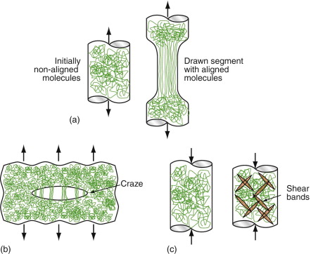
Figure 6.16 (a) Cold drawing—one of the mechanisms of deformation of thermoplastics.(b) Crazing—local drawing across a crack. (c) Shear banding.
Many polymers, among them PE, PP and nylon, draw at room temperature. Others with higher glass temperatures, such as PMMA, do not, although they draw well at higher temperatures. At room temperature they craze. Small crack-shaped regions within the polymer draw down. Because the crack has a larger volume than the polymer that was there to start with, the drawn material ends up as ligaments that link the craze surfaces, as in Figure 6.16(b). Crazes scatter light, so their presence causes whitening, easily visible when cheap plastic articles are bent. If stretching is continued, one or more crazes develop into proper cracks, and the sample fractures.
When crazing limits ductility in tension, large plastic strains may still be possible in compression by shear banding (Figure 6.16(c)). Within each band, shear takes place with much the same consequences for the shape of the sample as shear by dislocation motion. Continued compression causes the number of shear bands to increase, giving increased overall strain.
6.5 Manipulating strength
Strengthening metals
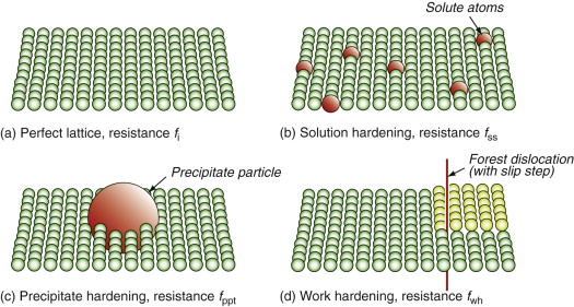
The way to make crystalline materials stronger is to make it harder for dislocations to move. As we have seen, dislocations move in a pure crystal when the force τb per unit length exceeds the lattice resistance fi. There is little we can do to change this—it is an intrinsic property like the modulus E. Other strengthening mechanisms add to it, and here there is scope for manipulation. Figure 6.17 introduces them. It shows the view of a slip plane from the perspective of an advancing dislocation: each strengthening mechanism presents a new obstacle course. In the perfect lattice shown in (a) the only resistance is the intrinsic strength of the crystal; solution hardening, shown in (b), introduces atom-size obstacles to motion; precipitation hardening, shown in (c), presents larger obstacles; and in work hardening, shown in (d), the slip plane becomes stepped and threaded with ‘forest’ dislocations.
Obstacles to dislocation motion increase the resistance f and thus the strength. To calculate their contribution to f, there are just two things we need to know about them: their spacing and their strength. Spacing means the distance L between them in the slip plane. The number of obstacles touching unit length of dislocation line is then

Each individual obstacle exerts a pinning force p on the dislocation line—a resisting force per unit length of dislocation—so the contribution of the obstacles to the resistance f is

Thus, the added contribution to the shear stress τ needed to make the dislocation move is (from equation (6.8))

The pinning is an elastic effect—it derives from the fact that both the dislocation and the obstacle distort the lattice elastically even though, when the dislocation moves, it produces plastic deformation. Because of this p, for any given obstacle in any given material, scales as Eb2, which has the units of force. The shear stress τ needed to force the dislocation through the field of obstacles then has the form

where α is a dimensionless constant characterizing the obstacle strength.
Armed with this background we can explain strengthening mechanisms. We start with solid solutions.
Solution hardening
Solid solution hardening is strengthening by deliberate additions of impurities or, more properly said, by alloying (Figure 6.18(a)). The addition of zinc to copper makes the alloy brass—copper dissolves up to 30% zinc. The zinc atoms replace copper atoms to form a random substitutional solid solution. The zinc atoms are bigger that those of copper and, in squeezing into the copper lattice, they distort it. This roughens the slip plane, so to speak, making it harder for dislocations to move, thereby adding an additional resistance fss, opposing dislocation motion. The figure illustrates that the concentration of solute, expressed as an atom fraction, is on average:
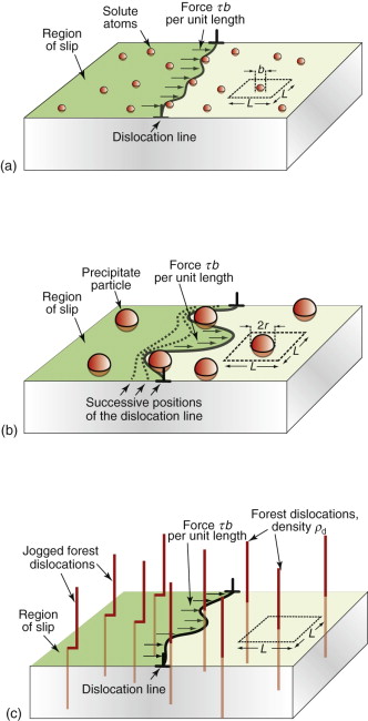
Figure 6.18 (a) Solution hardening. (b) Precipitation or dispersion hardening. (c) Forest hardening (work hardening).

where L is the spacing of obstacles in the slip plane and b is the atom size. Thus,

Plugging this into equation (6.11) relates the contribution of solid solution to the shear stress required to move the dislocation:
τss increases as the square root of the solute concentration. Brass, bronze and stainless steels, and many other metallic alloys, derive their strength in this way. They differ only in the extent to which the solute distorts the crystal, described by the constant α.
Dispersion and precipitate strengthening
A more effective way to impede dislocations is to disperse small, strong particles in their path. One way to make such a microstructure is to disperse small solid particles of a high melting point compound into a liquid metal, and to cast it to shape, trapping the particles in place—it is the way that metal–matrix composites such as Al–SiC are made. An alternative is to form the particles in situ by a precipitation process. If a solute (copper, say) is dissolved in a metal (aluminum, for instance) at high temperature when both are molten, and the alloy is solidified and cooled to room temperature, the solute precipitates as small particles, much as salt will crystallize from a saturated solution when it is cooled. An alloy of aluminum containing 4% copper, treated in this way, gives very small, closely spaced precipitates of the hard compound CuAl2. Copper alloyed with a little beryllium, similarly treated, gives precipitates of the compound CuBe. Most steels are strengthened by precipitates of carbides, obtained in this way. The precipitates give a large contribution to f.
Figure 6.18(b) shows how particles obstruct dislocation motion. If the particles are too strong for the dislocation to slice through them, the force τb pushes the dislocation between them, bending it to a tighter and tighter radius against its line tension (equation (6.9)). The radius is at a minimum when it reaches half the particle spacing, L; after that it can expand under lower stress. It is a bit like blowing up a bicycle inner tube when the outer tire has a hole in it: once you reach the pressure that balloons the inner tube through the hole, the balloon needs a smaller pressure to get bigger still. The critical configuration is the semicircular one: here the total force τbL on one segment of length L is just balanced by the force 2T due to the line tension (equation (6.10)), acting on either side of the bulge, as in Figure 6.19. The dislocation escapes when
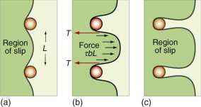
Figure 6.19 Successive positions of a dislocation as it bypasses particles that obstruct its motion. The critical configuration is that with the tightest curvature, shown in (b).
The obstacles thus exert a resistance of fppt = 2T/L. Precipitation hardening is an effective way to increasing strength: precipitate-hardened aluminum alloys can be 15 times stronger than pure aluminum.
Example 6.3
A polycrystalline aluminum alloy contains a dispersion of hard particles of diameter 10−8 m and an average centre-to-centre spacing of 6 × 10⁻⁸ m, measured in the slip planes. The Young’s modulus of aluminum is E = 70 GPa and b = 0.286 nm. Estimate the contribution of the hard particles to the yield strength of the alloy.
Answer. For the alloy, L = (6 − 1) × 10−8 m = 5 × 10⁻⁸ m, giving
Work hardening
The rising part of the stress–strain curve of Figure 6.1 is caused by work hardening: it is caused by the accumulation of dislocations generated by plastic deformation. The dislocation density, ρd, is defined as the length of dislocation line per unit volume (m/m3). Even in an annealed soft metal, the dislocation density is around 1010 m/m3, meaning that a 1 cm cube (the size of a cube of sugar) contains about 10 km of dislocation line. When metals are deformed, dislocations multiply, causing their density to grow to as much as 1017 m/m3 or more—100 million km per cubic centimeter. A moving dislocation now finds that its slip plane is penetrated by a forest of intersecting dislocations with an average spacing L = ρd−1/2 (since ρd is a number per unit area). Figure 6.18(c) suggests the picture. If a moving dislocation advances, it shears the material above the slip plane relative to that below, and that creates a little step called a jog in each forest dislocation. The jogs have potential energy—they are tiny segments of dislocation of length b—with the result that each exerts a pinning force p = Eb2/2 on the moving dislocation. Assembling these results into equation (6.10) gives
The greater the density of dislocations, the smaller the spacing between them, and so the greater their contribution to τwh.
All metals work harden. It can be a nuisance: if you want to roll thin sheet, work hardening quickly raises the yield strength so much that you have to stop and anneal the metal (heat it up to remove the accumulated dislocations) before you can go on—a trick known to blacksmiths for centuries. But it is also useful: it is a potent strengthening method, particularly for alloys that cannot be heat-treated to give precipitation hardening.
Example 6.4
A cube of the aluminum in Example 6.3 has a side length 1 cm and a dislocation density of 108 mm−2. Assuming a square array of parallel dislocations, estimate: (a) the total length of dislocation in the sample; (b) the distance between dislocations; (c) the contribution of the dislocations to the strength of the crystal.
- (a) The dislocation density ρd is the length of dislocation per unit volume. For a 1 cm cube, volume = 1000 mm3. Dislocation density = 108 mm−2 (mm/mm3), hence total length of dislocation = 108 × 1000 = 1011 mm = 100 000 km!
- (b) Assume that the dislocations form a uniform square array of side d. In this case, each dislocation sits at the centre of an area d2. For a unit length of dislocation, the volume of material per dislocation is 1 × d2, so the dislocation density is ρd = 1/d2, hence
- (c) From equation (6.14)
Grain boundary hardening
Almost all metals are polycrystalline, made up of tiny, randomly oriented crystals, or grains, meeting at grain boundaries like those of Figure 6.10(d). The grain size, D, is typically 10–100 µm. These boundaries obstruct dislocation motion. A dislocation in one grain—call it grain 1—can’t just slide into the next (grain 2) because the slip planes don’t line up. Instead, new dislocations have to nucleate in grain 2 with slip vectors that, if superimposed, match that of the dislocation in grain 1 so that the displacements match at the boundary. This gives another contribution to strength, τgb, that is found to scale as D−1/2, giving

where kp is called the Petch constant, after the man who first measured it. For normal grain sizes τgb is small and not a significant source of strength, but for materials that are microcrystalline (D < 1 µm) or nanocrystalline (D approaching 1 nm) it becomes significant.
Relationship between dislocation strength and yield strength
To a first approximation the strengthening mechanisms add up, giving a shear yield strength, τy, of
Strong materials either have a high intrinsic strength, τi (like diamond), or they rely on the superposition of solid solution strengthening τss, precipitates τppt and work hardening τwh (like high-tensile steels). Nanocrystalline solids exploit, in addition, the contribution of τgb.
Before we can use this information, one problem remains: we have calculated the yield strength of one crystal, loaded in shear. We want the yield strength of a polycrystalline material in tension. To link them there are two simple steps. First, a uniform tensile stress σ creates a shear stress on planes that lie at an angle to the tensile axis; dislocations will first move on the slip plane on which this shear stress is greatest. Figure 6.20 shows how this is calculated. A tensile force F acting on a rod of cross-section A, if resolved parallel to a plane with a normal that lies at an angle θ to the axis of tension, gives a force F sin θ in the plane. The area of this plane is A/cos θ, so the shear stress is
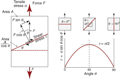
Figure 6.20 The resolution of stress. A tensile stress σ gives a maximum shear stress τ = σ/2 on a plane at 45 degree to the tensile axis.
where σ = F/A is the tensile stress. The value of τ is plotted against θ in the figure. The maximum lies at an angle of 45 degrees, when τ = σ/2.
Second, when this shear stress acts on an aggregate of crystals, some crystals will have their slip planes oriented favorably with respect to the shear stress, others will not. This randomness of orientation jacks up the strength by a further factor of 1.5 (called the Taylor factor—see the footnote on p. 122). Combining these results, the tensile stress to cause yielding of a sample that has many grains is approximately three times the shear strength of a single crystal:
Thus, the superposition of strengthening mechanisms in equation (6.16) applies equally to the yield strength, σy.
Strength and ductility of alloys
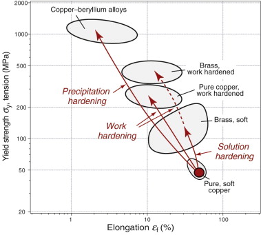
Of all the properties that materials scientists and engineers have sought to manipulate, the strength of metals and alloys is probably the most explored. It is easy to see why—Table 6.1 gives a small selection of the applications of metals and their alloys. Their importance in engineering design is enormous. The hardening mechanisms often are used in combination. This is illustrated graphically for copper alloys in Figure 6.21. Good things, however, have to be paid for. Here the payment for increased strength is, almost always, loss of ductility so the elongation εf is reduced. The material is stronger but it cannot be deformed as much without fracture.
Table 6.1 Metal alloys with typical applications, indicating the strengthening mechanisms used
| Alloy | Typical uses | Solution hardening | Precipitation hardening | Work hardening |
|---|---|---|---|---|
| Pure Al | Kitchen foil | ✓✓✓ | ||
| Pure Cu | Wire | ✓✓✓ | ||
| Cast Al, Mg | Automotive parts | ✓✓✓ | ✓ | |
| Bronze (Cu–Sn), Brass (Cu–Zn) | Marine components | ✓✓✓ | ✓ | ✓✓ |
| Non-heat-treatable wrought Al | Ships, cans, structures | ✓✓✓ | ✓✓✓ | |
| Heat-treatable wrought Al | Aircraft, structures | ✓ | ✓✓✓ | ✓ |
| Low-carbon steels | Car bodies, structures, ships, cans | ✓✓✓ | ✓✓✓ | |
| Low alloy steels | Automotive parts, tools | ✓ | ✓✓✓ | ✓ |
| Stainless steels | Pressure vessels | ✓✓✓ | ✓ | ✓✓✓ |
| Cast Ni alloys | Jet engine turbines | ✓✓✓ | ✓✓✓ |
Symbols: ✓✓✓ = Routinely used. ✓ = Sometimes used.
Strengthening polymers
In non-crystalline solids the dislocation is not a helpful concept. We think instead of some unit step of the flow process: the relative slippage of two segments of a polymer chain, or the shear of a small molecular cluster in a glass network. Their strength has the same origin as that underlying the lattice resistance: if the unit step involves breaking strong bonds (as in an inorganic glass), the materials will be strong and brittle, as ceramics are. If it only involves the rupture of weak bonds (the Van der Waals bonds in polymers, for example), it will be weak. Polymers too must therefore be strengthened by impeding the slippage of segments of their molecular chains. This is achieved by blending, by drawing, by cross-linking and by reinforcement with particles, fibres or fabrics.
A blend is a mixture of two polymers, stirred together in a sort of industrial food-mixer. The strength and modulus of a blend are just the average of those of the components, weighted by volume fraction (a rule of mixtures again). If one of these is a low molecular weight hydrocarbon, it acts as a plasticiser, reducing the modulus and giving the blend a leather-like flexibility.
Drawing is the deliberate use of the molecule-aligning effect of stretching, like that sketched in Figure 6.16(a), to greatly increase stiffness and strength in the direction of stretch. Fishing line is drawn nylon, Mylar film is a polyester with molecules aligned parallel to the film and geotextiles, used to restrain earth banks, are made from drawn polyethylene.
Cross-linking, sketched in Figures 4.18 and 4.19, creates strong bonds between molecules that were previously linked by weak Van der Waals forces. Vulcanized rubber is rubber that has been cross-linked, and the superior strength of epoxies derives from cross-linking.
Reinforcement is possible with particles of cheap fillers—sand, talc or wood dust. Far more effective is reinforcement with fibres—usually glass or carbon—either continuous or chopped, as explained in Chapter 4.
6.6 Summary and conclusions
Load-bearing structures require materials with reliable, reproducible strength. There is more than one measure of strength. Elastic design requires that no part of the structure suffers plastic deformation, and this means that the stresses in it must nowhere exceed the yield strength, σy, of ductile materials or the elastic limit of those that are not ductile. Plastic design, by contrast, allows some parts of the structure to deform plastically so long as the structure as a whole does not collapse. Then two further properties become relevant: the ductility, εf, and the tensile strength, σts, which are the maximum strain and the maximum stress the material can tolerate before fracture. The tensile strength is generally larger than the yield strength because of work hardening.
Charts plotting strength, like those plotting modulus, show that material families occupy different areas of material property space, depending on the strengthening mechanisms on which they rely. Crystal defects—particularly dislocations—are central to the understanding of these. It is the motion of dislocations that gives plastic flow in crystalline solids, giving them unexpectedly low strengths. When strength is needed it has to be provided by the strengthening mechanism that impedes dislocation motion.
First among these is the lattice resistance—the intrinsic resistance of the crystal to dislocation motion. Others can be deliberately introduced by alloying and heat treatment. Solid solution hardening, dispersion and precipitation hardening, work hardening and grain boundary hardening add to the lattice resistance. The strongest materials combine them all.
Noncrystalline solids—particularly polymers—deform in a less organised way by the pulling of the tangled polymer chains into alignment with the direction of deformation. This leads to cold drawing with substantial plastic strain and, at lower temperatures, to crazing. The stress required to do this is significant, giving polymers a considerable intrinsic strength. This can be enhanced by blending, cross-linking and reinforcement with particles or fibres to give the engineering polymers we use today.
Ashby M.F., Jones D.R.H. Engineering Materials Vols. I–II 2006 Butterworth-Heinemann Oxford, UK ISBN 7-7506-6380-4 and ISBN 0-7506-6381-2. (An introduction to mechanical properties and processing of materials.)
Cottrell A.H. Dislocations and Plastic Flow in Crystals 1953 Oxford University Press Oxford, UK (Long out of print but worth a search: the book that first presented a coherent picture of the mechanisms of plastic flow and hardening.)
Friedel J. Dislocations 1964 Addison-Wesley Reading, MA, USA Library of Congress No. 65-21133. (A book that, with that of Cottrell, first established the theory of dislocations.)
Hertzberg R.W. Deformation and Fracture of Engineering Materials 3rd ed. 1989 Wiley New York, USA ISBN 0-471-61722-9. (A readable and detailed coverage of deformation, fracture and fatigue.)
Hull D., Bacon D.J. Introduction to Dislocations 4th ed. 2001 Butterworth-Heinemann Oxford, UK ISBN 0-750-064681-0. (An introduction to dislocation mechanics.)
Hull D., Clyne T.W. An Introduction to Composite Materials 2nd ed. 1996 Cambridge University Press Cambridge, UK ISBN 0-521-38855-4. (A concise and readable introduction to composites that takes an approach that minimises the mathematics and maximises the physical understanding.)
Young R.J. Introduction to Polymers 1981 Chapman & Hall London, UK ISBN 0-412-22180-2. (A good starting point for more information on the chemistry, structure and properties of polymers.)
6.8 Exercises
- Exercise E6.1 Sketch a stress–strain curve for a typical metal. Mark on it the yield strength σy, the tensile strength σts and the ductility εf. Indicate on it the work done per unit volume in deforming the material up to a strain of ε, εf (pick your own strain ε).
- Exercise E6.2 What is meant by the ideal strength of a solid? Which material class most closely approaches it?
- Exercise E6.3 Use the yield strength–density chart or the yield strength–modulus chart (Figures 6.6 and 6.7) to find:
- The metal with the lowest strength.
- The approximate range of strength of the composite GFRP.
- Whether there are any polymers that are stronger than wood measured parallel to the grain.
- How the strength of GFRP compares with that of wood.
- Whether elastomers, that have moduli that are far lower than polymers, are also far lower in strength.
- Exercise E6.4 The lattice resistance of copper, like that of most FCC metals, is small. When 10% of nickel is dissolved in copper to make a solid solution, the strength of the alloy is 150 MPa. What would you expect the strength of an alloy with 20% nickel to be?
- Exercise E6.5 A metal–matrix composite consists of aluminum containing hard particles of silicon carbide (SiC) with a mean spacing of 3 µm. The composite has a strength of 180 MPa. If a new grade of the composite with a particle spacing of 2 µm were developed, what would you expect its strength to be?
- Exercise E6.6 Nanocrystalline materials have grain sizes in the range 0.01–0.1 µm. If the contribution of grain boundary strengthening in an alloy with grains of 0.1 µm is 20 MPa, what would you expect it to be if the grain size were reduced to 0.01 µm?
- Exercise E6.7 Polycarbonate, PC (yield strength 70 MPa) is blended with polyester (PET; yield strength 50 MPa) in the ratio 30%/70%. If the strength of blends follows a rule of mixtures, what would you expect the yield strength of this blend to be?
6.9 Exploring design with CES (use Level 2 Materials unless otherwise suggested)
- Exercise E6.8 Find, by opening the records, the yield strengths of copper, brass (a solid solution of zinc in copper) and bronze (a solid solution of tin in copper). Report the mean values of the ranges that appear in the records. What explains the range within each record, since the composition is not a variable? What explains the differences in the mean values, when composition is a variable?
- Exercise E6.9 Use a ‘Limit’ stage to find materials with a yield strength σy greater than 100 MPa and density ρ less than 2000 kg/m3. List the results.
- Exercise E6.10 Add two further constraints to the selection of the previous exercise. Require now that the material price be less than 5 $/kg and the elongation be greater than 5%.
- Exercise E6.11 Use the CES Level 3 database to select Polypropylene and its blended, filled and reinforced grades. To do so, open CES Edu Level 3, apply a ‘Tree’ stage selecting Polymers—Thermoplastics—Polypropylene (folder). Make a chart with Young’s modulus E on the x-axis and yield strength σy on the y-axis. Label the records on the chart by clicking on them. Explain, as far as you can, the trends you see.
- Exercise E6.12 Apply the same procedure as that of the last exercise to explore copper and its alloys. Again, use your current knowledge to comment on the origins of the trends.
6.10 Exploring the science with CES Elements
- Exercise E6.13 The elastic (potential) energy per unit length of a dislocation is 0.5 Eb2 J/m. Make a bar chart of the energy stored in the form of dislocations, for a dislocation density of 1014 m/m3. Assume that the magnitude of Burger’s vector, b, is the same as the atomic diameter. (You will need to use the ‘Advanced’ facility in the axis-choice dialog box to make the function.) How do the energies compare with the cohesive energy, typically 5 × 10⁴ MJ/m3
- Exercise E6.14 Work hardening causes dislocations to be stored. Dislocations disrupt the crystal and have potential energy associated with them. It has been suggested that sufficient work hardening might disrupt the crystal so much that it becomes amorphous. To do this, the energy associated with the dislocations would have to be about equal to the heat of fusion, since this is the difference in energy between the ordered crystal and the disordered liquid. The energy per unit length of a dislocation is 0.5 Eb2 J/m. Explore this in the following way:
- (a) Calculate and plot the energy associated with a very high dislocation density of 1017 m/m3 for the elements, i.e. plot a bar chart of 0.5 × 10¹⁷ Eb2 on the y-axis using twice atomic radius as equal to Burger’s vector b. Remember that you must convert GPa into kPa and atomic radius from nm to m to get the energy in kJ/m3.
- (b) Now add, on the x-axis, the heat of fusion energy. Convert it from kJ/mol to kJ/m3 by multiplying Hc by 1000/molar volume, with molar volume in m3/kmol (as it is in the database). What, approximately, is the ratio of the dislocation energy to the energy of fusion? Would you expect this very high dislocation density to be enough to make the material turn amorphous?
1Thomas Telford (1757–1834), Scottish engineer, brilliant proponent of the suspension bridge at a time when its safety was a matter of debate. Telford may himself have had doubts—he was given to lengthy prayer on the days that the suspension chains were scheduled to take the weight of the bridge. Most of his bridges, however, still stand.
2Isambard Kingdom Brunel (1806–1859), perhaps the greatest engineer of the Industrial Revolution (c. 1760–1860) in terms of design ability, personality, power of execution and sheer willingness to take risks—the Great Eastern, for example, was five times larger than any previous ship ever built. He took the view that ‘great things are not done by those who simply count the cost’. Brunel was a short man and self-conscious about his height; he favored tall top hats to make himself look taller.
3Geoffrey (G. I.) Taylor (1886–1975), known for his many fundamental contributions to aerodynamics, hydrodynamics and to the structure and plasticity of metals—it was he, with Egon Orowan, who realised that the ductility of metals implied the presence of dislocations. One of the greatest of contributors to theoretical mechanics and hydrodynamics of the 20th century, he was also a supremely practical man—a sailor himself, he invented (among other things) the anchor used by the Royal Navy.
4Egon Orowan (1901–1989), Hungarian/US physicist and metallurgist, who, with G. I. Taylor, realised that the plasticity of crystals could be understood as the motion of dislocations. In his later years he sought to apply these ideas to the movement of fault lines during earthquakes.