Chapter 20 Materials, processes and the environment
- 20.1 Introduction and synopsis 504
- 20.2 Material consumption and its growth 504
- 20.3 The material life cycle and criteria for assessment 507
- 20.4 Definitions and measurement: embodied energy, process energy and end of life potential 509
- 20.5 Charts for embodied energy 513
- 20.6 Design: selecting materials for eco-design 515
- 20.7 Summary and conclusions 520
- 20.8 Appendix: some useful quantities 521
- 20.9 Further reading 522
- 20.10 Exercises 522
- 20.11 Exploring design with CES 524
The practice of engineering consumes vast quantities of materials and is dependent on a continuous supply of them. We start by surveying this consumption, emphasising the materials used in the greatest quantities. Increasing population and living standards cause this consumption rate to grow—something it cannot do forever. Finding ways to use materials more efficiently is a prerequisite for a sustainable future.
20.1 Introduction and synopsis
The practice of engineering consumes vast quantities of materials and is dependent on a continuous supply of them. We start by surveying this consumption, emphasising the materials used in the greatest quantities. Increasing population and living standards cause this consumption rate to grow—something it cannot do forever. Finding ways to use materials more efficiently is a prerequisite for a sustainable future.
There is a more immediate problem: present-day material usage already imposes stress on the environment in which we live. The environment has some capacity to cope with this, so that a certain level of impact can be absorbed without lasting damage. But it is clear that current human activities exceed this threshold with increasing frequency, diminishing the quality of the world in which we now live and threatening the well-being of future generations. Design for the environment is generally interpreted as the effort to adjust our present product design efforts to correct known, measurable, environmental degradation; the time-scale of this thinking is 10 years or so, an average product’s expected life. Design for sustainability is the longer-term view: that of adaptation to a lifestyle that meets present needs without compromising the needs of future generations. The time-scale here is less clear—it is measured in decades or centuries—and the adaptation required is much greater.
20.2 Material consumption and its growth
Material consumption
Speaking globally, we consume roughly 10 billion (1010) tonnes of engineering materials per year. Figure 20.1 gives a perspective: it is a bar chart of the consumption of the materials used in the greatest quantities. It has some interesting messages. On the extreme left, for calibration, are hydrocarbon fuels—oil and coal—of which we currently consume a colossal 9 billion tonnes per year. Next, moving to the right, are metals. The scale is logarithmic, making it appear that the consumption of steel (the first metal) is only a little greater than that of aluminum (the next); in reality, the consumption of steel exceeds, by a factor of 10, that of all other metals combined. Steel may lack the high-tech image that attaches to materials like titanium, carbon-fibre-reinforced composites and (most recently) nano-materials, but make no mistake, its versatility, strength, toughness, low cost and wide availability are unmatched.
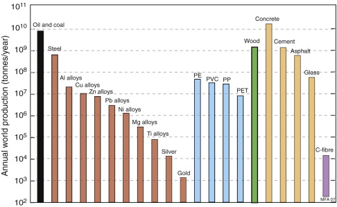
Figure 20.1 The consumption of hydrocarbons (left-hand column) and of engineering materials (the other columns).
Polymers come next: 50 years ago their consumption was tiny; today the combined consumption of commodity polymers polyethylene (PE), polyvinyl chloride (PVC), polypropylene (PP) and polyethylene-terephthalate (PET) begins to approach that of steel.
The really big ones, though, are the materials of the construction industry. Steel is one of these, but the consumption of wood for construction purposes exceeds that of steel even when measured in tonnes per year (as in the diagram), and since it is a factor of 10 lighter, if measured in m3/year, wood totally eclipses steel. Bigger still is the consumption of concrete, which exceeds that of all other materials combined. The other big ones are asphalt (roads) and glass.
The last column of all illustrates things to come: it shows today’s consumption of carbon fibre. Just 20 years ago this material would not have crept onto the bottom of this chart. Today its consumption is approaching that of titanium and is growing fast.
The columns in this figure describe broad classes of materials, so—out of the 160 000 materials now available—they probably include 99.9% of all consumption when measured in tonnes. This is important when we come to consider the impact of materials on the environment, since impact scales with consumption.
The growth of consumption
Most materials are being consumed at a rate that is growing exponentially with time (Figure 20.2), simply because both population and living standards grow exponentially. One consequence of this is dramatised by the following statement: at a global growth rate of just 3% per year we will mine, process and dispose of more ‘stuff’ in the next 25 years than in the entire history of human engineering (see Exercises). If the current rate of consumption in tonnes per year is C then exponential growth means that
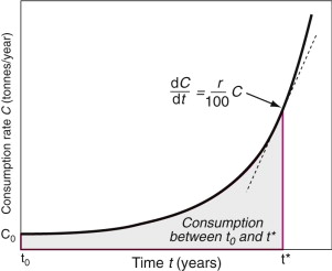
Figure 20.2 Exponential growth. Consumption rate C doubles in a time td ≈ 70/r, where r is the annual growth rate.
where, for the generally small growth rates we deal with here (1–5% per year), r can be thought of as the percentage fractional rate of growth per year. Integrating over time gives

where C0 is the consumption rate at time t = t0. The doubling time tD of consumption rate is given by setting C/C0 = 2 to give
After a period of stagnation, steel consumption is growing again, driven by growth in China; at 4% per year it doubles about every 18 years. Polymer consumption is rising at about 5% per year—it doubles every 14 years. During times of boom—the 1960s and 1970s, for instance—polymer production increased much faster than this, peaking at 18% per year (it doubled every 4 years).
Example 20.1
A total of 5 million cars were sold in China in 2007; in 2008 the sale was 6.6 million. What is the annual growth rate of car sales, expressed as % per year? If there were 15 million cars already on Chinese roads by the end of 2007 and this growth rate continues, how many cars will there be in 2020, assuming that the number that are removed from the roads in this time interval can be neglected?
Answer. Starting with equation (20.2)
we enter C = 6.6 × 10⁶ and C0 = 5 × 10⁶ and the time interval (t − t0) = 1 year, and solve for r. The result is r = 27.8% per year.
The cumulative number of cars entering use in the subsequent 13 years is found from the integral of this equation over time
Entering C0 = 5 × 10⁶ (the number in 2007), r = 27.8% per year and (t* − t0) = 13 gives the additional number of cars by 2020 at Qt* = 650 × 106. To this (if we are picky) we must add the number already there in 2007, giving a final total of 655 × 106—half a billion—an increase on the number in 2007 by a factor of 100. (This colossal number is still only equivalent to 1 car per 3-person family, less than the current car ownership per family in the United States.)
The picture, then, is one of a global economy ever more dependent on a supply of materials, almost all drawn from non-renewable resources. To manage these in a sustainable way requires an understanding of the material life cycle. We turn to this next.
20.3 The material life cycle and criteria for assessment
Life-cycle assessment and energy
The materials life cycle is sketched in Figure 20.3. Ore and feedstock, drawn from the earth’s resources, are processed to give materials; these are manufactured into products that are used and, at the end of their lives, discarded, a fraction perhaps entering a recycling loop, the rest committed to incineration or landfill. Energy and materials are consumed at each point in this cycle (we shall call them ‘phases’), with an associated penalty of CO2, SOx, NOx and other emissions—heat, and gaseous, liquid and solid waste, collectively called environmental ‘stressors’. These are assessed by the technique of life-cycle analysis (LCA). A rigorous LCA examines the life cycle of a product and assesses in detail the eco-impact created by one or more of its phases of life, cataloging and quantifying the stressors. This requires information for the life history of the product at a level of precision that is available only after the product has been manufactured and used. It is a tool for the evaluation and comparison of existing products, rather than one that guides the design of those that are new.
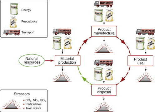
Figure 20.3 The material life cycle. Ore and feedstock are mined and processed to yield a material. This is manufactured into a product that is used and, at the end of its life, discarded or recycled. Energy and materials are consumed in each phase, generating waste heat and solid, liquid and gaseous emissions.
A full LCA is time-consuming and expensive, and it cannot cope with the problem that 80% of the environmental burden of a product is determined in the early stages of design, when many decisions are still fluid. This has led to the development of more approximate ‘streamline’ LCA methods that seek to combine acceptable cost with sufficient accuracy to guide decision-making, the choice of materials being one of these decisions. But even then there is a problem: a designer, seeking to cope with many interdependent decisions that any design involves, inevitably finds it hard to know how best to use data of this type. How are CO2 and SOx emissions to be balanced against resource depletion, toxicity or ease of recycling?
This perception has led to efforts to condense the eco-information about a material production into a single measure or indicator, normalising and weighting each source of stress to give the designer a simple, numeric ranking. The use of a single-valued indicator is criticised by some. The grounds for criticism are that there is no agreement on normalisation or weighting factors, and that the method is opaque since the indicator value has no simple physical significance. But on one point there is international agreement: the Kyoto Protocol of 1997 committed the developed nations that signed it to progressively reduce carbon emissions, meaning CO2. At the national level the focus is more on reducing energy consumption, but since this and CO2 production are closely related, they are nearly equivalent. Thus, there is a certain logic in basing design decisions on energy consumption or CO2 generation; they carry more conviction than the use of a more obscure indicator. We shall follow this route, using energy as our measure. Before doing this, we provide some definitions.
20.4 Definitions and measurement: embodied energy, process energy and end of life potential
Embodied energy Hm and CO2 footprint
The embodied energy of a material is the energy that must be committed to create 1 kg of usable material—1 kg of steel stock, or of PET pellets or of cement powder, for example—measured in MJ/kg. The CO2 footprint is the associated release of CO2, in kg/kg. It is tempting to try to estimate embodied energy via the thermodynamics of the processes involved—extracting aluminum from its oxide, for instance, requires the provision of the free energy of oxidation to liberate it. This much energy must be provided, it is true, but it is only the beginning. The thermodynamic efficiencies of processes are low, seldom reaching 50%. Only part of the output is usable—the scrap fraction ranges from a few per cent to more than 10%. The feedstocks used in the extraction or production themselves carry embodied energy. Transport is involved. The production plant itself has to be lit, heated and serviced. And if it is a dedicated plant, one that is built for the sole purpose of making the material or product, there is an ‘energy mortgage’—the energy consumed in building the plant in the first place.
Embodied energies are more properly assessed by input–output analysis. For example, for a material such as ingot iron, cement powder or PET granules, the embodied energy/kg is found by monitoring over a fixed period of time the total energy input to the production plant (including that smuggled in, so to speak, as embodied energy of feedstock) and dividing this by the quantity of usable material shipped out of the plant. The upper part of Figure 20.4 shows, much simplified, the inputs to a PET production facility: oil derivatives such as naphtha and other feedstock, direct power (which, if electric, is generated with a production efficiency of about 34%) and the energy of transporting the feedstock to the facility. The plant has an hourly output of usable PET granules. The embodied energy of the PET, (Hm)PET, with usual units of MJ/kg, is then given by
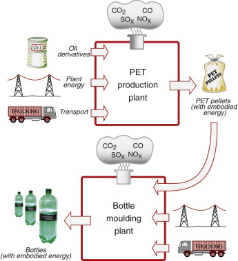
Figure 20.4 An input–output diagram for PET production (giving the embodied energy/kg of PET) and for bottle production (giving the embodied energy/bottle).
The processing energy Hp associated with a material is the energy, in MJ, used to shape, join and finish 1 kg of the material to create a component or product. Thus polymers, typically, are moulded or extruded; metals are cast, forged or machined; ceramics are shaped by powder methods. A characteristic energy per kg is associated with each of these. Continuing with the PET example, the granules now become the input (after transportation) to a facility for blow-moulding PET bottles for water, as shown in the lower part of Figure 20.4. There is no need to list the inputs again—they are broadly the same, the PET itself bringing with it its embodied energy (Hm)PET. The output of the analysis is the energy committed per bottle produced.
There are many more steps before the bottle reaches a consumer and is drunk: collection, filtration and monitoring of the water, transportation of water and bottles to bottling plant, labeling, delivery to central warehouse, distribution to retailers and refrigeration prior to sale. All have energy inputs, which, when totalled, give the energy cost of as simple a thing as a plastic bottle of cold water.
The end of life potential summarises the possible utility of the material at life’s end: the ability to be recycled back into the product from which it came, the lesser ability to be down-cycled into a lower-grade application, the ability to be biodegraded into usable compost, the ability to yield energy by controlled combustion and, failing all of these, the ability to be buried as landfill without contaminating the surrounding land then or in the future.
Recycling: ideals and realities
We buy, use and discard paper, packaging, cans, bottles, television sets, computers, furniture, tires, cars, even buildings. Why not retrieve the materials they contain and use them again? What could be simpler?
If you think that, think again. First, some facts. There are (simplifying again) two sorts of ‘scrap’, by which we mean material with recycle potential. In-house scrap is the off-cuts, ends and bits left in a material production facility when the usable material is shipped out. Here ideals are realised: almost 100% is recycled, meaning that it goes back into the primary production loop. But once a material is released into the outside world the picture changes. It is processed to make parts that may be small, very numerous and widely dispersed; it is assembled into products that contain many other materials; it may be painted, printed or plated; and its subsequent use contaminates it further. To reuse it, it must be collected (not always easy), separated from other materials, identified, decontaminated, chopped and processed. Collection is time-intensive and this makes it expensive. Imperfect separation causes problems: even a little copper or tin damages the properties of steel; residual iron embrittles aluminum; heavy metals (lead, cadmium, mercury) are unacceptable in many alloys; PVC contamination renders PET unusable, and dyes, water and almost any alien plastic render a polymer unacceptable for its original demanding purpose, meaning that it can be used only in less demanding applications (a fate known as ‘down-cycling’).
Despite these difficulties, recycling can be economic, both in cash and energy terms. This is particularly so for metals: the energy commitment per kg for recycled aluminum is about one-tenth of that for virgin material; that for steel is about one-third. Some inevitable contamination is countered by addition of virgin material to dilute it. Metal recycling is both economic and makes important contributions to the saving of energy.
The picture for plastics is less rosy. The upper part of Figure 20.5 illustrates this for PET. Bottles are collected and delivered to the recycling plant as mixed plastic—predominantly PET, but with PE and PP bottles too. Table 20.1 lists the steps required to recycle the PET, each one consuming energy, with the results listed in Table 20.2. Some energy is saved, but not a lot—typically 50%.
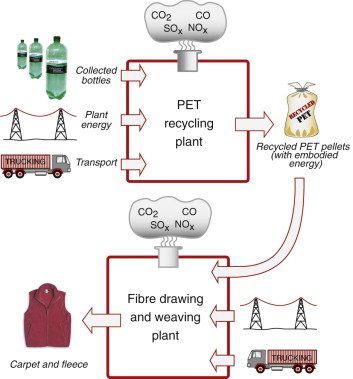
Figure 20.5 A simplified input–output diagram for the recycling of plastics to recover PET, and its use to make lower-grade products such as fleece.
Table 20.1 The energy-absorbing steps in recycling PET
Table 20.2 Embodied energy and market price of virgin and recycled plastics
| Polymer | Embodied energy* (MJ/kg) | Price† ($/kg) | ||
|---|---|---|---|---|
| Virgin | Recycled | Virgin | Recycled | |
| HDPE | 82 | 40 | 1.9 | 0.9 |
| PP | 82 | 40 | 1.8 | 1.0 |
| PET | 85 | 55 | 2.0 | 1.1 |
| PS | 101 | 45 | 1.5 | 0.8 |
| PVC | 66 | 37 | 1.4 | 0.9 |
* Approximate values; see CES Edu software for details.
Recycling of PET, then, can offer an energy saving. But is it economic? Time, in manufacture, is money. Collection, inspection, separation and drying are slow processes, and every minute adds dollars to the cost. Add to this the fact that the quality of recycled material is less good than the original, limiting its use to less demanding products, as suggested by the lower part of Figure 20.5—recycled PET cannot be used for bottles. Table 20.2 lists the current market price of granules of five commodity polymers in the virgin and the recycled states. If the recycled stuff were as good as new it would command the same price; in reality it commands little more than half. Thus, using today’s technology, the cost of recycling plastics is high and the price they command is low, not a happy combination.
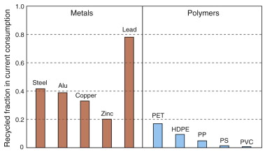
The consequences of this are brought out by Figure 20.6. It shows the current recycle fraction of commodity metals and plastics. The recycle fraction is the fraction of current supply that derives from recycling. For metals it is high: most of the lead, and almost half the steel and one-third of the aluminum we use today have been used at least once before. For plastics the only small success is PET, with a recycle fraction of about 18%, but for the rest the contribution is tiny, for many zero. Oil price inflation and restrictive legislation could change all this, but for the moment, that is how it is.
The energy demands of products
With this background, we can proceed to look at the way products consume energy in each of the four life phases of Figure 20.3. The procedure is to tabulate the main components of the product together with their material and weight. The embodied energy and energy of processing associated with the product are estimated by multiplying the weights by the energies Hm and Hp, and summing. The use-energy of energy-using products may be estimated from information for the power, the duty cycle and the source from which the power is drawn. To this should be added the energy associated with maintenance and service over the useful life of the product. The energy of disposal is more difficult: some energy may be recovered by incineration, some saved by recycling, but, as already mentioned, there is also an energy cost associated with collection and disassembly. Transport costs can be estimated from the distance of transport and the energy/km.kg of the transport mode used.
Despite the uncertainty in some of the data, the outcome of this analysis is revealing. Figure 20.7 presents the evidence for a range of product groups. It has two significant features, with important implications. The product groups in the top row all consume energy as an unavoidable consequence of their use and for these the use-phase overwhelmingly dominates the life energy. The products in the bottom row depend less heavily on energy but are material intensive; for these it is the embodied energy of the material that dominates. If large changes are to be achieved, it is the dominant phase that must be the first target; when the differences are as great as those shown here, a reduction in the others makes little impact on the total, and the precision of the data for Hm and Hp is not the issue—an error of a factor of 2 changes the outcome very little. It is in the nature of those who conduct detailed LCA studies to wish to do so with precision, and better data are always a desirable goal. But engineers and designers need the ability to move forward without it, recognising that precise judgements can be drawn from imprecise data.
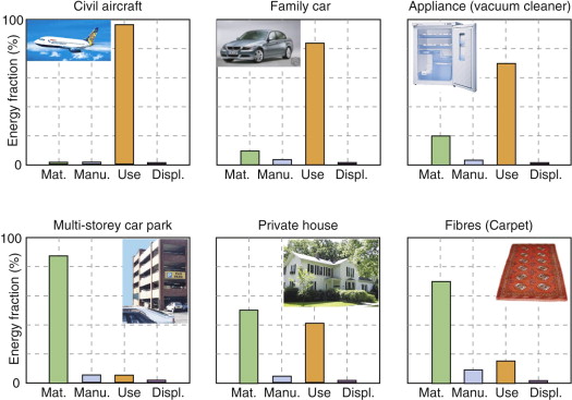
Figure 20.7 Approximate values for the energy consumed at each phase of Figure 20.3 for a range of products. The columns show the approximate embodied energy (‘Mat.’), energy to manufacture (‘Manu.’), use energy over design life (‘Use’) and energy for disposal (’Displ.’).
20.5 Charts for embodied energy
Bar charts for embodied energy
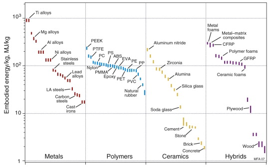
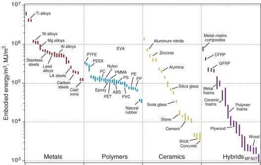
Figures 20.8 and 20.9 show the embodied energy per kg and per m3 for materials. When compared per unit mass, metals, particularly steels, appear as attractive choices, demanding much less energy than polymers. But when compared on a volume basis, the ranking changes and polymers lie lower than metals. The light alloys based on aluminum, magnesium and titanium are particularly demanding, with energies that are high by either measure. This prompts the question: what measure should we choose to make meaningful comparisons if we wish to minimise the embodied energy of a product? The answer is the same as the one we used with the objectives of minimising mass or cost: it is to minimise embodied energy per unit of function. To do that we need the next two charts.
Property charts for embodied energy in structural design
Earlier chapters discussed the property trade-offs in problems of structural design. The function of the design might be, for example, to support a load without too much deflection, or without failure, while minimising the mass. For this, modulus–density or strength–density were used. If the objective becomes minimising the energy embodied in the material of the product while providing structural functionality, we need equivalent charts for these.
Figures 20.10 and 20.11 are a pair of materials selection charts for minimising energy Hm per unit stiffness and strength. The first shows modulus E plotted against Hmρ; the guidelines give the slopes for three of the commonest performance indices. The second shows strength σy plotted against Hmρ; again, guidelines give the slopes. The two charts give survey data for minimum energy design. They are used in exactly the same way as the E–ρ and σy–ρ charts for minimum mass design.

Figure 20.10 The modulus–embodied energy chart made with the CES software. It is the equivalent of the E–ρ chart of Figure 4.6 and is used in the same way.
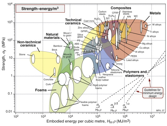
Figure 20.11 The strength–embodied energy chart made with the CES software. It is the equivalent of the σy–ρ chart of Figure 6.6 and is used in the same way.
20.6 Design: selecting materials for eco-design
For selection of materials in environmentally responsible design we must first ask: which phase of the life cycle of the product under consideration makes the largest impact on the environment? The answer guides the effective use of the data in the way shown in Figure 20.12.
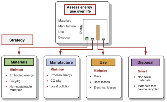
Figure 20.12 Rational use of the database starts with an analysis of the phase of life to be targeted. The decision then guides the method of selection to minimise the impact of the phase on the environment.
The material production phase
If material production consumes more energy than the other phases of life, it becomes the first target. Drink containers provide an example: they consume materials and energy during material extraction and container production, but, apart from transport and possible refrigeration, not thereafter. Here, selecting materials with low embodied energy and using less of them are the ways forward. Figure 20.7 made the point that large civil structures—buildings, bridges, roads—are material intensive. For these the embodied energy of the materials is the largest commitment. For this reason architects and civil engineers concern themselves with embodied energy as well as the thermal efficiency of their structures.
The product manufacture phase
The energy required to shape a material is usually much less than that to create it in the first place. Certainly it is important to save energy in production. But higher priority often attaches to the local impact of emissions and toxic waste during manufacture, and this depends crucially on local circumstances. Clean manufacture is the answer here.
The product use phase
The eco-impact of the use phase of energy-using products has nothing to do with the embodied energy of the materials themselves—indeed, minimising this may frequently have the opposite effect on use energy. Use energy depends on mechanical, thermal and electrical efficiencies; it is minimised by maximising these.
Fuel efficiency in transport systems (measured, say, by MJ/km) correlates closely with the mass of the vehicle itself; the objective then becomes that of minimising mass. The evidence for this can be seen in Figure 20.13, showing the fuel consumption of some 4000 European models of car against their unladen mass, segregated by engine type (super-sport and luxury cars, shown as red symbols, are separated out—for these, fuel economy is not a design priority). The lines show linear fits through the data: the lowest, through the green symbols, for diesel-powered cars, the one above, through the blue symbols, for those with petrol engines. One hybrid model is included (yellow symbol). The correlation between fuel consumption and weight is clear. Here the solution is minimum mass design, discussed extensively in earlier chapters; it is just as relevant to eco-design as to performance-driven design.
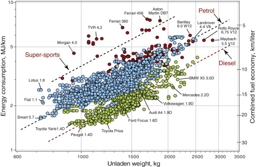
Figure 20.13 Energy consumption and fuel economy of 2005 model European cars, plotted against the unladen weight. The open red symbols are diesels, the open black are petrol driven and the full red symbols are for cars designed with performance, above all else, in mind. The broken lines are best fits to data for each type. Note the near-linear dependence of energy consumption on weight.
Energy efficiency in refrigeration or heating systems is achieved by minimising the heat flux into or out of the system; the objective is then that of minimising thermal conductivity or thermal inertia. Energy efficiency in electrical generation, transmission and conversion is maximised by minimising the ohmic losses in the conductor; here the objective is to minimise electrical resistance while meeting necessary constraints on strength, cost and so on. Material selection to meet these objectives is well documented in other chapters and the texts listed under Further reading.
The product disposal phase
The environmental consequences of the final phase of product life have many aspects. The ideal is summarised in the following guidelines:
- Avoid toxic materials such as heavy metals and organometallic compounds that, in landfill, cause long-term contamination of soil and groundwater.
- Examine the use of materials that cannot be recycled, since recycling can save both material and energy, but keep in mind the influence they have on the other phases of life.
- Seek to maximise recycling of materials for which this is possible, even though recycling may be difficult to achieve for the reasons already discussed.
- When recycling is impractical seek to recover energy by controlled combustion.
- Consider the use of materials that are biodegradable or photo-degradable, although these are ineffectual in landfill because the anaerobic conditions within them inhibit rather than promote degradation.
Implementing this requires information for toxicity, potential for recycling, controlled combustion and biodegradability. The CES software provides simple checks of each of these.
Case study: crash barriers
Barriers to protect driver and passengers of road vehicles are of two types: those that are static (the central divider of a freeway, for instance) and those that move (the fender of the vehicle itself) (Figure 20.14). The static type lines tens of thousands of miles of road. Once in place they consume no energy, create no CO2 and last a long time. The dominant phases of their life in the sense of Figure 20.7 are those of material production and manufacture. The fender, by contrast, is part of the vehicle; it adds to its weight and thus to its fuel consumption. The dominant phase here is that of use. This means that, if eco-design is the objective, the criteria for selecting materials for the two sorts of barrier will differ.
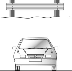
Figure 20.14 Two crash barriers, one static, the other—the fender—attached to something that moves. Different eco-criteria are needed for each.
The function of a barrier is to transfer load from the point of impact to the support structure, where reaction from the foundation or from crush elements in the vehicle support or absorb it. To do this the material of the barrier must have adequate strength, σy, and the ability to be shaped and joined cheaply, and (thinking of the disposal phase of life) recyclable. That for the car fender must meet these constraints with minimum mass, since this will reduce the use energy. As we know from Chapter 7, this means materials with high values of the index

where σy is the tensile strength and ρ is its density. For the static barrier embodied energy, not weight, is the problem. If we change the objective to that of minimum embodied energy, we require materials with large values of
where Hm is the embodied energy per kg of material.
The chart of Figure 7.8 guides selection for the mobile barrier, where we seek strength at low weight. CFRPs excel by this criterion, but they are not recyclable. Heavier, but recyclable, are alloys of magnesium, titanium and aluminum. Ceramics are excluded both by their brittleness and the difficulty of shaping and joining them.
The chart of Figure 20.11 guides the selection for static barriers, where we seek strength at low embodied energy. The index M2 is plotted in Figure 20.15. The chart shows that embodied energy per unit strength (leaving ceramics aside because of brittleness) is minimised by making the barrier from carbon steel, cast iron or wood; nothing else comes close.
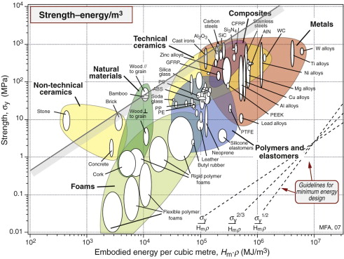
Figure 20.15 The selection of materials for strength at minimum embodied energy. The best choices (rejecting ceramics because they are brittle) are cast iron, steel and wood.
Stiffness-limited design is treated in a similar way. Achieving it at minimum mass was the subject of Chapters 4 and 5. To do so at minimum embodied energy just requires that ρ is replaced by Hmρ.
20.7 Summary and conclusions
Rational selection of materials to meet environmental objectives starts by identifying the phase of product life that causes greatest concern: production, manufacture, use or disposal. Dealing with all of these requires data not only for the obvious eco-attributes (energy, CO2 and other emissions, toxicity, ability to be recycled and the like) but also data for mechanical, thermal, electrical and chemical properties. Thus, if material production is the phase of concern, selection is based on minimising the embodied energy or the associated emissions (CO2 production, for example). But if it is the use phase that is of concern, selection is based instead on low weight, or excellence as a thermal insulator, or as an electrical conductor while meeting other constraints on stiffness, strength, cost and so on. The charts of this book give guidance in meeting these constraints and objectives. The CES databases provide data and tools that allow more sophisticated selection.
20.8 Appendix: some useful quantities
-
Coal, lignite 15–19 MJ/kg Coal, anthracite 31–34 MJ/kg Oil 11.69 kWh/liter = 47.3 MJ/kg Gas 10.42 kWh/m3 LPG 13.7 kWh/liter = 46.5–49.6 MJ/kg
Approximate energy requirements of transport systems in MJ per tonne-km
-
Sea freight 0.11 Barge (river freight) 0.83 Rail freight 0.86 Truck 0.9–1.5, depending on size of truck (large are more economic) Air freight 8.3–15, depending on type and size of plane
Ashby M.F. Materials Selection in Mechanical Design 3rd ed. 2005 Butterworth-Heinemann Oxford, UK ISBN 0-7506-6168-2. (A more advanced text developing the ideas presented here.)
Brundlandt D. Report of the World Commission on the Environment and Development 1987 Oxford University Press Oxford, UK ISBN 0-19-282080-X. (A much quoted report that introduced the need and potential difficulties of ensuring a sustainable future.)
Dieter G.E. Engineering Design, A Materials and Processing Approach 2nd ed. 1991 McGraw-Hill New York, USA ISBN 0-07-100829-2. (A well-balanced and respected text focusing on the place of materials and processing in technical design.)
Goedkoop M., Effting S., Collignon M. The Eco-indicator 99: A Damage Oriented Method for Life Cycle Impact Assessment, Manual for Designers (14 April 2000) http://www.pre.nl 2000 (An introduction to eco-indicators, a technique for rolling all the damaging aspects of material production into a single number.)
Graedel T.E. Streamlined Life-cycle Assessment 1998 Prentice-Hall New Jersey, USA ISBN 0-13-607425-1. (An introduction to LCA methods and ways of streamlining them.)
Kyoto Protocol (1997). United Nations, Framework Convention on Climate Change. Document FCCC/CP1997/7/ADD.1 〈http://cop5.unfccc.de〉 O 14040/14041/14042/14043, ‘Environmental management—life cycle assessment’ and subsections, Geneva, Switzerland. (The international consensus on combating climate change.)
20.10 E xercises
- Exercise E20.1 What is meant by embodied energy per kilogram of a metal? Why does it differ from the thermodynamic energy of formation of the oxide, sulfide or silicate from which it was extracted?
- Exercise E20.2 What is meant by the process energy per kilogram for casting a metal? Why does it differ from the latent heat of melting of the metal?
- Exercise E20.3 Why is the recycling of metals more successful than that of polymers?
- Exercise E20.4 The world consumption rate of CFRP is rising at 8% per year. How long does it take to double?
- Exercise E20.5 Prove the statement made in the text that, ‘at a global growth rate of just 3% per year we will mine, process and dispose of more ‘stuff’ in the next 25 years than in the entire history of human engineering.’ For the purpose of your proof, assume consumption started with the dawn of the Industrial Revolution, 1750.
Exercise E20.6 Which phase of life would you expect to be the most energy intensive (in the sense of consuming fossil fuel) for the following products:
Exercise E20.7 Show that the index for selecting materials for a strong panel, loaded in bending, with the minimum embodied energy content is:
- Exercise E20.8 Use the E–Hmρ chart of Figure 20.10 to find the metal with a modulus E greater than 100 GPa and the lowest embodied energy per unit volume.
- Exercise E20.9 Use the chart of σy–Hmρ (Figure 20.11) to find material for strong panels with minimum embodied energy per unit volume.
- Exercise E20.10 Car fenders used to be made of steel. Most cars now have extruded aluminum or glass-reinforced polymer fenders. Both materials have a much higher embodied energy than steel. Take the mass of a steel bumper to be 20 kg and that of an aluminum one to be 14 kg; a bumper-set (two bumpers) weighs twice as much. Find an equation for the energy consumption in MJ/km as a function of mass for petrol engine cars using the data plotted in Figure 20.13.
- (a) Work out how much energy is saved by changing the bumper-set of a 1500 kg car from steel to aluminum.
- (b) Calculate whether, over an assumed life of 200 000 km, the switch from steel to aluminum has saved energy. You will find the embodied energies of steel and aluminum in the CES Level 2 database. Ignore the differences in energy in manufacturing the two bumpers—it is small. (The energy content of gasoline is 44 MJ/litre.)
- (c) The switch from steel to aluminum increases the price of the car by $60. Using current pump prices for gasoline, work out whether, over the assumed life, it is cheaper to have the aluminum fender or the steel one.

20.11 E xploring design with CES
- Exercise E20.11 Rank the three common commodity materials Low carbon steel, Age hardening aluminum alloy and Polyethylene by embodied energy/kg and embodied energy/m3, using data drawn from Level 2 of the CES Edu database (use the means of the ranges given in the databases). Materials in products perform a primary function—providing stiffness, strength, heat transfer and the like. What is the appropriate measure of embodied energy for a given function?
Exercise E20.12 Plot a bar chart for the embodied energies of metals and compare it with one for polymers, on a ‘per unit yield strength’ basis, using CES. You will need to use the ‘Advanced’ facility in the axis-selection window to make the function:
Exercise E20.13 Drink containers co-exist that are made from a number of different materials. The masses of five competing container types, the material of which they are made and the specific energy content of each are listed in the following table. Which container type carries the lowest overall embodied energy per unit of fluid contained?
Container type Material Mass (g) Embodied energy (MJ/kg) PET 400 ml bottle PET 25 84 PE 1 litre milk bottle High-density PE 38 80 Glass 750 ml bottle Soda glass 325 14 Al 440 ml can 5000 series Al alloy 20 200 Steel 440 ml can Plain carbon steel 45 23 - Exercise E20.14 Iron is made by the reduction of iron oxide, Fe2O3, with carbon, aluminum by the electrochemical reduction of bauxite, basically Al2O3. The enthalpy of oxidation of iron to its oxide is 5.5 MJ/kg, that of aluminum to its oxide is 20.5 MJ/kg. Compare these with the embodied energies of cast iron and of carbon steel, and of aluminum, retrieved from the CES database (use means of the ranges given there). What conclusions do you draw?
- Exercise E20.15 Calculate the energy to mold PET by assuming it to be equal to the energy required to heat PET from room temperature to its melting temperature, Tm. Compare this with the actual moulding energy. You will find the moulding energy, the specific heat and the melting temperature in the Level 2 record for PET in CES (use means of the ranges). Assume that the latent heat of melting is equal to that to raise the temperature from room temperature to the melting point. What conclusions do you draw?