
Chapter 4 Stiffness and weight: Density and elastic moduli
- 4.1 Introduction and synopsis 48
- 4.2 Density, stress, strain and moduli 48
- 4.3 The big picture: material property charts 57
- 4.4 The science: what determines density and stiffness? 59
- 4.5 Manipulating the modulus and density 70
- 4.6 Summary and conclusions 73
- 4.7 Further reading 75
- 4.8 Exercises 75
- 4.9 Exploring design with CES 77
- 4.10 Exploring the science with CES Elements 78
Stress causes strain. If you are human, the ability to cope with stress without undue strain is called resilience. If you are a material, it is called elastic modulus.
4.1 Introduction and synopsis
Stress causes strain. If you are human, the ability to cope with stress without undue strain is called resilience. If you are a material, it is called elastic modulus.
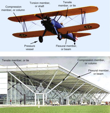
Stress is something that is applied to a material by loading it. Strain—a change of shape—is its response; it depends on the magnitude of the stress and the way it is applied—the mode of loading. The cover picture illustrates the common ones. Ties carry tension—often, they are cables. Columns carry compression—tubes are more efficient as columns than solid rods because they don’t buckle as easily. Beams carry bending moments, like the wing spar of the plane or the horizontal roof beams of the airport. Shafts carry torsion, as in the drive shaft of cars or the propeller shaft of the plane. Pressure vessels contain a pressure, as in the tires of the plane. Often they are shells: curved, thin-walled structures.
Stiffness is the resistance to change of shape that is elastic, meaning that the material returns to its original shape when the stress is removed. Strength (Chapter 6) is its resistance to permanent distortion or total failure. Stress and strain are not material properties; they describe a stimulus and a response. Stiffness (measured by the elastic modulus E, defined in a moment) and strength (measured by the elastic limit σy or tensile strength σts) are material properties. Stiffness and strength are central to mechanical design, often in combination with the density, ρ. This chapter introduces stress and strain and the elastic moduli that relate them. These properties are neatly summarised in a material property chart—the modulus–density chart—the first of many that we shall explore in this book.
Density and elastic moduli reflect the mass of the atoms, the way they are packed in a material and the stiffness of the bonds that hold them together. There is not much you can do to change any of these, so the density and moduli of pure materials cannot be manipulated at all. If you want to control these properties you can either mix materials together, making composites, or disperse space within them, making foams. Property charts are a good way to show how this works.
4.2 Density, stress, strain and moduli
Density
Many applications (e.g. sports equipment, transport systems) require low weight and this depends in part on the density of the materials of which they are made. Density is mass per unit volume. It is measured in kg/m3 or sometimes, for convenience, Mg/m3 (1 Mg/m3 = 1000 kg/m3).
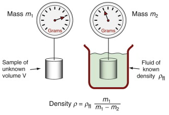
The density of samples with regular shapes can be determined using precision mass balance and accurate measurements of the dimensions (to give the volume), but this is not the best way. Better is the ‘double weighing’ method: the sample is first weighed in air and then when fully immersed in a liquid of known density. When immersed, the sample feels an upward force equal to the weight of liquid it displaces (Archimedes’ principle1). The density is then calculated as shown in Figure 4.1.
Modes of loading
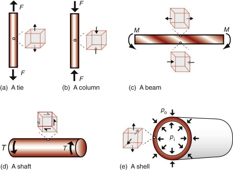
Most engineering components carry loads. Their elastic response depends on the way the loads are applied. As explained earlier, the components in both structures shown on the cover are designed to withstand different modes of loading: tension, compression, bending, torsion and internal pressure. Usually one mode dominates, and the component can be idealised as one of the simply loaded cases in Figure 4.2—tie, column, beam, shaft or shell. Ties carry simple axial tension, shown in (a); columns do the same in simple compression, as in (b). Bending of a beam (c) creates simple axial tension in elements on one side the neutral axis (the center-line, for a beam with a symmetric cross-section) and simple compression in those on the other. Shafts carry twisting or torsion (d), which generates shear rather than axial load. Pressure difference applied to a shell, like the cylindrical tube shown in (e), generates bi-axial tension or compression.
Stress
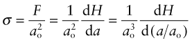
Consider a force F applied normal to the face of an element of material, as in Figure 4.3 on the left of row (a). The force is transmitted through the element and balanced by an equal but opposite force on the other side, so that it is in equilibrium (it does not move). Every plane normal to F carries the force. If the area of such a plane is A, the tensile stress σ in the element (neglecting its own weight) is
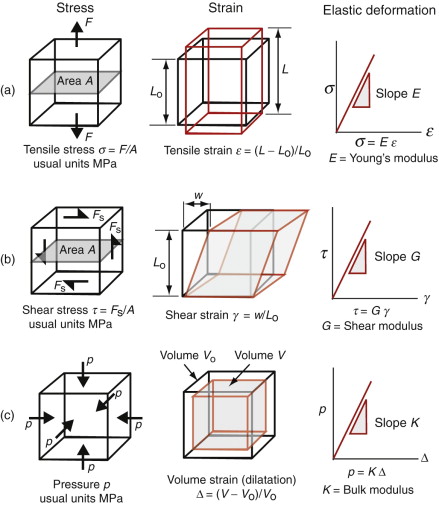

If the sign of F is reversed, the stress is compressive and given a negative sign. Forces2 are measured in newtons (N), so stress has the dimensions of N/m2. But a stress of 1 N/m2 is tiny—atmospheric pressure is 105 N/m2—so the usual unit is MN/m2 (106 N/m2), called megapascals, symbol MPa3.
Example 4.1
A brick chimney is 50 m tall. The bricks have a density of ρ = 1800 kg/m3. What is the axial compressive stress at its base? Does the shape of the cross-section matter?
Answer. Let the cross-section area of the chimney be A and its height be h. The weight of the chimney is F = ρAhg, where g is the acceleration due to gravity. Using equation (4.1), the axial compressive stress at the base is σ = −F/A = −ρgh where the ‘−’ indicates compression (the area A has cancelled out). This is the same formula as for the static pressure at depth h in a fluid of density ρ. The stress is independent of the shape or size of the cross-section. Assuming g = 10 m/s2, σ = −1800 × 10 × 50 = −9 × 10⁵ N/m2 = −0.9 MPa.
If, instead, the force lies parallel to the face of the element, three other forces are needed to maintain equilibrium (Figure 4.3, row (b)). They create a state of shear in the element. The shaded plane, for instance, carries the shear stress τ of

The units, as before, are MPa.
One further state of multi-axial stress is useful in defining the elastic response of materials: that produced by applying equal tensile or compressive forces to all six faces of a cubic element, as in Figure 4.3, row (c). Any plane in the cube now carries the same state of stress—it is equal to the force on a cube face divided by its area. The state of stress is one of hydrostatic pressure, symbol p, again with the units of MPa. There is an unfortunate convention here. Pressures are positive when they push—the reverse of the convention for simple tension and compression.
Engineering components can have complex shapes and can be loaded in many ways, creating complex distributions of stress. But no matter how complex, the stresses in any small element within the component can always be described by a combination of tension, compression and shear. Commonly the simple cases of Figure 4.3 suffice, using superposition of two cases to capture, for example, bending plus compression.
Strain
Strain is the response of materials to stress (second column of Figure 4.3). A tensile stress σ applied to an element causes the element to stretch. If the element in Figure 4.3(a), originally of side Lo, stretches by δL = L − Lo, the nominal tensile strain is

A compressive stress shortens the element; the nominal compressive strain (negative) is defined in the same way. Since strain is the ratio of two lengths, it is dimensionless.
A shear stress causes a shear strain γ (Figure 4.3(b)). If the element shears by a distance w, the shear strain
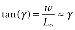
In practice tan γ ≈ γ because strains are almost always small. Finally, a hydrostatic pressure p causes an element of volume V to change in volume by δV. The volumetric strain, or dilatation (Figure 4.3(c)), is

Stress–strain curves and moduli
Figure 4.4 shows typical tensile stress–strain curves for a ceramic, a metal and a polymer. The initial part, up to the elastic limit σel, is approximately linear (Hooke’s4 law), and it is elastic, meaning that the strain is recoverable—the material returns to its original shape when the stress is removed. Stresses above the elastic limit cause permanent deformation (ductile behavior) or brittle fracture.
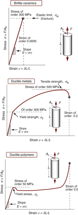
Within the linear elastic regime, strain is proportional to stress (Figure 4.3, third column). The tensile strain is proportional to the tensile stress:
and the same is true in compression. The constant of proportionality, E, is called Young’s5 modulus. Similarly, the shear strain γ is proportional to the shear stress τ:
and the dilatation Δ is proportional to the pressure p:
where G is the shear modulus and K the bulk modulus, as illustrated in the third column of Figure 4.3. All three of these moduli have the same dimensions as stress, that of force per unit area (N/m2 or Pa). As with stress it is convenient to use a larger unit, this time an even bigger one, that of 109 N/m2, gigapascals, or GPa.
Young’s modulus, the shear modulus and the bulk modulus are related, but to relate them we need one more quantity, Poisson’s6 ratio. When stretched in one direction, the element of Figure 4.3(a) generally contracts in the other two directions, as it is shown doing here. Poisson’s ratio, ν, is the negative of the ratio of the lateral or transverse strain, εt, to the axial strain, ε, in tensile loading:

Since the transverse strain itself is negative, ν is positive—it is typically about 1/3.
Example 4.2
The chimney in Example 4.1 has bricks with Young’s modulus E = 25 GPa, and Poisson’s ratio ν = 0.2. What are the axial and transverse strains at the bottom of the chimney?
Answer. Using the result of Example 4.1 with equation (4.6), the axial strain is ε = σ / E = −9 × 10⁵/25 × 109 = −3.6 × 10⁻⁵ (often written as 36 microstrain, µε). From equation (4.9), the transverse strain is εt = −νε = 7.2 µε. This time the strain is positive, indicating a small expansion at the base of the chimney.
In an isotropic material (one for which the moduli do not depend on the direction in which the load is applied) the moduli are related in the following ways:
Elastomers are exceptional. For these ν ≈ 1/2 when
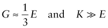
This means that rubber (an elastomer) is easy to stretch in tension (low E), but if constrained from changing shape, or loaded hydrostatically, it is very stiff (large K)—a feature for which designers of shoes have to allow.
Data sources like CES list values for all four moduli. In this book we examine data for E; approximate values for the others can be derived from equations (4.11a) and (4.11b) when needed.
Elastic energy
If you stretch an elastic band, energy is stored in it. The energy can be considerable: catapults can kill people. The super-weapon of the Roman arsenal at one time was a wind-up mechanism that stored enough elastic energy to hurl a 10 kg stone projectile 100 yards or more.
How do you calculate this energy? A force F acting through a displacement dL does work F dL. A stress σ = F/A acting through a strain increment dε = dL/L does work per unit volume
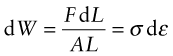
with units of J/m3. If the stress is acting on an elastic material, this work is stored as elastic energy. The elastic part of all three stress–strain curves of Figure 4.4—the part of the curve before the elastic limit—is linear; in it σ = Eε. The work done per unit volume as the stress is raised from zero to a final value σ* is the area under the stress–strain curve:
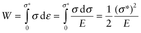
This is the energy that is stored, per unit volume, in an elastically strained material. The energy is released when the stress is relaxed.
Example 4.3
A steel rod has length Lo = 10 m and a diameter d = 10 mm. The steel has Young’s modulus E = 200 GPa, elastic limit (the highest stress at which it is still elastic and has not yielded) σe = 500 MPa and density ρ = 7800 kg/m3. Calculate the force in the rod, its extension and the elastic energy per unit volume it stores when it is stretched so that the stress in it just reaches the elastic limit. Compare the elastic energy per unit mass with the chemical energy stored in gasoline, which has a heat of combustion (calorific value) of 43 000 kJ/kg.
Answer. The cross-section area of the rod is A = πd2/4 = 7.85 × 10⁻⁵ m2.
At the elastic limit, the force in the rod is (4.1): F = σeA = 39.2 kN (3.92 tonnes).
The corresponding strain is (4.6): ε = σ/E = 500 × 106/200 × 109 = 0.0025 (i.e. 0.25%).
The extension of the rod is (4.3): δL = εLo = 0.0025 × 10 = 25 mm.
The elastic energy per unit volume, from equation (4.13), is W = σ2/2E = (500 × 106)2/(2 × 200 × 109) = 625 kJ/m3, giving an elastic energy per kg of W/ρ = 80 J/kg. This is less, by a factor of more than 500 000 than that of gasoline.
Measurement of Young’s modulus
You might think that the way to measure the elastic modulus of a material would be to apply a small stress (to be sure to remain in the linear elastic region of the stress–strain curve), measure the strain and divide one by the other. In reality, moduli measured as slopes of stress–strain curves are inaccurate, often by a factor of 2 or more, because of contributions to the strain from material creep or deflection of the test machine. Accurate moduli are measured dynamically: by measuring the frequency of natural vibrations of a beam or wire, or by measuring the velocity of sound waves in the material. Both depend on ![]() , so if you know the density ρ you can calculate E.
, so if you know the density ρ you can calculate E.
Stress-free strain
Stress is not the only stimulus that causes strain. Certain materials respond to a magnetic field by undergoing strain—an effect known as magneto-striction. Others respond to an electrostatic field in the same way—they are known as piezo-electric materials. In each case a material property relates the magnitude of the strain to the intensity of the stimulus (Figure 4.5). The strains are small but can be controlled with great accuracy and, in the case of magneto-striction and piezo-electric strain, can be changed with a very high frequency. This is exploited in precision positioning devices, acoustic generators and sensors—applications we return to in Chapters 14 and 15.
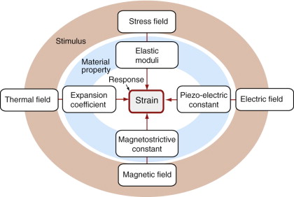
A more familiar effect is that of thermal expansion: strain caused by change of temperature. The thermal strain εT is linearly related to the temperature change ΔT by the expansion coefficient, α:
where the subscript T is a reminder that the strain is caused by temperature change, not stress.
The term ‘stress-free strain’ is a little misleading. It correctly conveys the idea that the strain is not caused by stress but by something else. But these strains can nonetheless give rise to stresses if the body suffering the strain is constrained. Thermal stress—stress arising from thermal expansion—particularly, can be a problem, causing mechanisms to jam and railway tracks to buckle. We analyse it in Chapter 12.
4.3 The big picture: material property charts
We met the idea of material property charts in Section 2.5. Now is the time to use them. If we want materials that are stiff and light, we first need an overview of what’s available. What moduli do materials offer? What are their densities? The modulus–density chart shows them.
The modulus–density chart
Figure 4.6 shows that the modulus E of engineering materials spans seven decades7, from 0.0001 to nearly 1000 GPa; the density ρ spans a factor of 2000, from less than 0.01 to 20 Mg/m3. The members of the ceramics and metals families have high moduli and densities; none has a modulus less than 10 GPa or a density less than 1.7 Mg/m3. Polymers, by contrast, all have moduli below 10 GPa and densities that are lower than those of any metal or ceramic—most are close to 1 Mg/m3. Elastomers have roughly the same density as other polymers but their moduli are lower by a further factor of 100 or more. Materials with a lower density than polymers are porous: man-made foams and natural cellular structures like wood and cork.
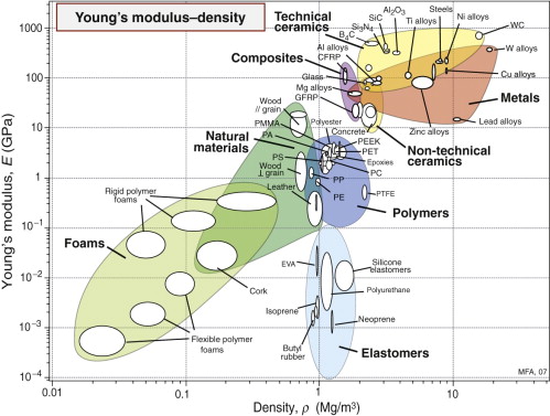
This property chart gives an overview, showing where families and their members lie in E–ρ space. It helps in the common problem of material selection for stiffness-limited applications in which weight must be minimised. Chapter 5 provides more on this.
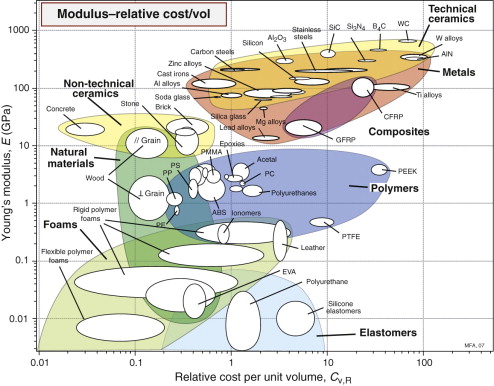
The modulus–relative cost chart
Often it is minimising cost, not weight, that is the overriding objective of a design. The chart of Figure 4.7 shows, on the x-axis, the relative prices per unit volume of materials, normalised to that of the metal used in larger quantities than any other: mild steel. Concrete and wood are among the cheapest; polymers, steels and aluminum alloys come next; special metals like titanium, most technical ceramics and a few polymers like PTFE and PEEK are expensive. The chart allows the selection of materials that are stiff and cheap. Chapter 5 gives examples.
Anisotropy
Glasses and most polymers have disordered structures with no particular directionality about the way the atoms are arranged. They have properties that are isotropic, meaning the same no matter which direction they are measured. Most materials are crystalline—made up of ordered arrays of atoms. Metals and ceramics are usually polycrystalline—made up of many tiny, randomly oriented crystals. This averages out the directionality in properties, so a single value is enough. Occasionally, though, anisotropy is important. Single crystals, drawn polymers and fibres are anisotropic; their properties depend on the direction in the material in which they are measured. Woods, for instance, are much stiffer along the grain than across it. Figures 4.6 and 4.7 have separate property bubbles for each of the two loading directions. Fibre composites are yet more extreme: the modulus parallel to the fibres can be larger by a factor of 20 than that perpendicular to them. Anisotropy must therefore be considered when wood and composite materials are selected.
4.4 The science: what determines density and stiffness?
Density
Atoms differ greatly in weight but little in size. Among solids, the heaviest stable atom, uranium (atomic weight 238), is about 35 times heavier than the lightest, lithium (atomic weight 6.9), yet when packed to form solids their diameters are almost exactly the same (0.32 nm). The largest atom, cesium, is only 2.5 times larger than the smallest, beryllium. Thus, the density is determined mainly by the atomic weight and is influenced to a lesser degree by the atoms’ size and the way in which they are packed. Metals are dense because they are made of heavy atoms, packed densely together (iron, for instance, has an atomic weight of 56). Polymers have low densities because they are largely made of light carbon (atomic weight: 12) and hydrogen (atomic weight: 1) in low-density amorphous or semi-crystalline packings. Ceramics, for the most part, have lower densities than metals because they contain light Si, O, N or C atoms. Even the lightest atoms, packed in the most open way, give solids with a density of around 1 Mg/m3—the same as that of water (see Figure 4.6). Materials with lower densities than this are foams, made up of cells containing a large fraction of pore space.
Atom packing in metals and the unit cell
Many of the properties of materials depend directly on the way the atoms or molecules within them are packed. In glasses the arrangement is a disordered one with no regularity or alignment. Most materials, however, are crystalline, with a regularly repeating pattern of structural units. Crystals are described using the language and methods of crystallography, which provides an elegant framework for thinking about their three-dimensional geometry. The ideas of crystallography are introduced briefly in the next five pages. Later in the book you will find the Guided Learning Unit 1: simple ideas of crystallography, which develops the ideas in greater depth. The rest of this chapter will be intelligible without reference to the unit, but working through it and its exercises will give a more complete understanding and confidence.
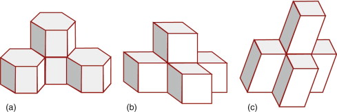
Atoms often behave as if they were hard, spherical balls. The balls on a pool table, when set, are arranged as a close-packed layer, as in Figure 4.8(a). The atoms of many metals pack in this way, forming layers that are far more extensive. There is no way to pack atoms more closely than this, so this particular arrangement is called ‘close packed’. Atomic structures are close packed not just in two dimensions but in three. Surprisingly, there are two ways to do this. The depressions where three atoms meet in the first layer, layer A, allow the closest nesting for a second layer, B. A third layer can be added such that its atoms are exactly above those in the first layer, so that it, too, is in the A orientation, and the sequence repeated to give a crystal with ABABAB … stacking, as in Figure 4.8(b); it is called close-packed hexagonal, or CPH (or sometimes HCP) for short, for reasons explained in a moment. There is also an alternative. In placing the second layer, layer B, there are two choices of position. If the third layer, C, is nested onto B so that it lies in the alternative position, the stacking becomes (on repeating) ABCABCABC … as shown in (c) in the figure; it is called face-centred cubic, or FCC, for short. Many metals, such as copper, silver, aluminum and nickel, have the FCC structure; many others, such as magnesium, zinc and titanium, have the CPH structure. The two alternative structures have exactly the same packing fraction, 0.74, meaning that the spheres occupy 74% of the available space. But the small difference in layout influences properties, particularly those to do with plastic deformation (Chapter 6).
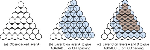
Figure 4.8 (a) A close-packed layer of spheres, layer A; atoms often behave as if hard and spherical. (b) A second layer, B, nesting in the first; repeating this sequence gives ABAB … or CPH stacking. (c) A third layer, C, can be nested so that it does not lie above A or B; if repeated this gives ABCABC … or FCC stacking.
Not all structures are close packed. Figure 4.9 shows one of these, made by stacking square-packed layers with a lower packing density than the hexagonal layers of the FCC and HCP structures. An ABABAB … stacking of these layers builds the body-centred cubic structure, BCC for short, with a packing fraction of 0.68. Iron and most steels have this structure. There are many other crystal structures, but for now these three are enough.
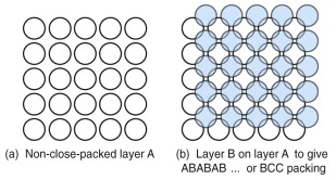
Figure 4.9 (a) A square grid of spheres; it is a less efficient packing than that of the previous figure. (b) A second layer, B, nesting in the first, A; repeating this sequence gives ABAB … packing. If the sphere spacing is adjusted so that the blue spheres lie on the corners of a cube, the result is the non-close-packed BCC structure.
Any regular packing of atoms that repeats itself is called a crystal. It is possible to pack atoms in a non-crystallographic way to give what is called an amorphous structure, sketched in Figure 4.10. This is not such an efficient way to fill space with spheres: the packing fraction is 0.64 at best.
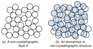
Figure 4.10 (a) An irregular arrangement of spheres. (b) Extending this in three dimensions gives a random or amorphous structure.
The characterising unit of a crystal structure is called its unit cell. Figure 4.11 shows three; the red lines define the cell (the atoms have been shrunk to reveal it more clearly). In the first, shown in (a), the cell is a hexagonal prism. The atoms in the top, bottom and central planes form close-packed layers like that of Figure 4.8(b), with ABAB … stacking. For these reasons, the structure is called close-packed hexagonal (CPH). The second, shown in (b), is also made up of close-packed layers, though this is harder to see: the shaded triangular plane is one of them. If we think of this as an A plane, atoms in the plane above it nest in the B position and those in the plane above that, in the C, giving ABCABC … stacking, as in Figure 4.8(c). The unit cell itself is a cube with an atom at each corner and one at the center of each face—for this reason it is called face-centred cubic (FCC). The final cell, shown in (c), is the characterising unit of the square-layer structure of Figure 4.9; it is a cube with an atom at each corner and one in the middle, and is called, appropriately, body-centred cubic (BCC).
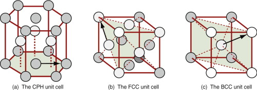
Figure 4.11 Unit cells. All the atoms are of the same type, but are shaded differently to emphasise their positions. (a) The close-packed hexagonal (CPH) structure. (b) The close-packed face-centred cubic (FCC) structure. (c) The non-close-packed body-centred cubic (BCC) structure. Arrows show nearest neighbors.
Unit cells pack to fill space as in Figure 4.12; the resulting array is called the crystal lattice; the points at which cell edges meet are called lattice points. The crystal itself is generated by attaching one or a group of atoms to each lattice point so that they form a regular, three-dimensional, repeating pattern. The cubic and hexagonal cells are among the simplest; there are many others with edges of differing lengths meeting at differing angles. The one thing they have in common is their ability to stack with identical cells to completely fill space.
Atom packing in ceramics
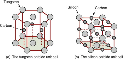
Most ceramics are compounds, made up of two or more atom types. They too have characteristic unit cells. Figure 4.13 shows those of two materials that appear on the charts: tungsten carbide (WC), and silicon carbide (SiC). The cell of the first is hexagonal, that of the second is cubic, but now a pair of different atoms is associated with each lattice point: a W—C pair in the first structure and an Si—C pair in the second.
Atom packing in glasses
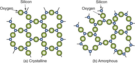
The crystalline state is the lowest energy state for elements and compounds. Melting disrupts the crystallinity, scrambling the atoms and destroying the regular order. The atoms in a molten metal look very like the amorphous structure of Figure 4.10. On cooling through the melting point most metals crystallise, though by cooling them exceedingly quickly it is sometimes possible to trap the molten structure to give an amorphous metallic ‘glass’. With compounds it is easier to do this, and with one in particular, silica—SiO2—crystallisation is so sluggish that its usual state is the amorphous one. Figure 4.14 shows, on the left, the atom arrangement in crystalline silica: identical hexagonal Si–O rings, regularly arranged. On the right is the more usual amorphous state. Now some rings have seven sides, some have six, some five, and there is no order—the next ring could be any one of these. Amorphous silica is the basis of almost all glasses; it is mixed with Na2O to make soda glass (windows, bottles) and with B2O5 to make borosilicate glasses (Pyrex), but it is the silica that gives the structure. It is for this reason that the structure itself is called ‘glassy’, a term used interchangeably with ‘amorphous’.
Atom packing in polymers
Polymer structures are quite different. The backbone of a ‘high’ polymer (‘high’ means high molecular weight) is a long chain of carbon atoms, to which side groups are attached. Figure 4.15 shows a segment of the simplest: polyethylene, PE, (—CH2—)n. The chains have ends; the ends of this one are capped with a CH3 group. PE is made by the polymerisation (snapping together) of ethylene molecules, CH2:CH2; the : symbol is a double bond, broken by polymerisation to give the links to more carbon neighbors to the left and right. Figure 4.16 shows the chain structure of five of the most widely used linear polymers.
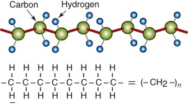
Figure 4.15 Polymer chains have a carbon–carbon backbone with hydrogen or other side groups. The figure shows three alternative representations of the polyethylene molecule.
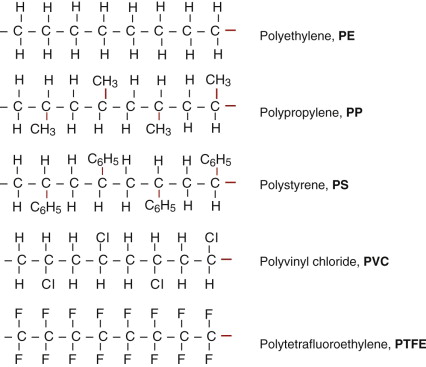
Figure 4.16 Five common polymers, showing the chemical make-up. The strong carbon–carbon bonds are shown in red.
Polymer molecules bond together to form solids. The chains of a linear polymer, 103 to 106 —CH2— units in length, are already strongly bonded along the chain itself. Separated chains attract each other, but weakly so (Figure 4.17(a))—they are sticky, but not very sticky; the ‘hydrogen’ bonds that make them stick are easily broken or rearranged. The resulting structure is sketched in Figure 4.18(a): a dense spaghetti-like tangle of molecules with no order or crystallinity; it is amorphous. This is the structure of thermoplastics like those of Figure 4.16; the weak bonds melt easily, allowing the polymer to be moulded, retaining its new shape on cooling.
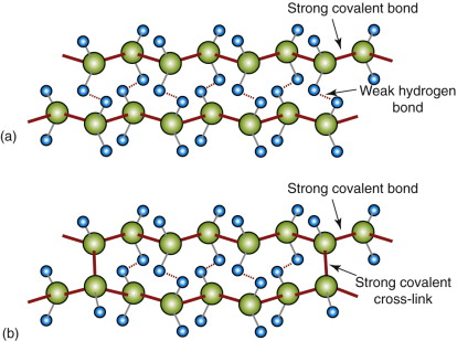
Figure 4.17 (a) Polymer chains have strong covalent ‘backbones’, but bond to each other only with weak hydrogen bonds unless they become cross-linked. (b) Cross-links bond the chains tightly together. The strong carbon–carbon bonds are shown as solid red lines.
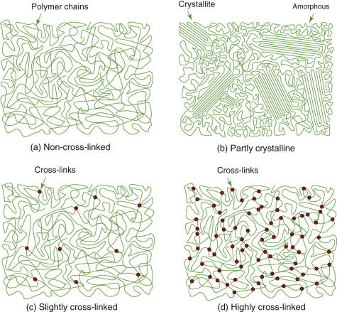
Figure 4.18 (a) Chains in polymers like polypropylene form spaghetti-like tangles with no regular repeating pattern—that structure is amorphous or ‘glassy’. (b) Some polymers have the ability to form regions in which the chains line up and register, giving crystalline patches. The sketch shows a partly crystalline polymer structure. (c) Elastomers have occasional cross-links between chains, but these are far apart, allowing the chains between them to stretch. (d) Heavily cross-linked polymers like epoxy inhibit chain sliding.
The weak bonds of thermoplastics, do, however, try to line molecules up, as they are shown in Figure 4.17(a). The molecules are so long that total alignment is not possible, but segments of molecules manage it, giving small crystalline regions, as in Figure 4.18(b). These crystallites, as they are called, are small—often between 1 and 10 μm across, just the right size to scatter light. So amorphous polymers with no crystallites can be transparent—polycarbonate (PC), polymethyl-methacrylate (PMMA; Plexiglas) and polystyrene (PS) are examples. Those with some crystallinity, like polyethylene (PE) and nylon (PA), scatter light and are translucent.
The real change comes when chains are cross-linked by replacing some of the weak hydrogen bonds by much more muscular covalent C—C bonds, as in Figure 4.17(b), making the whole array into one huge, multiply connected network. Elastomers (rubbery polymers) have relatively few cross-links, as in Figure 4.18(c). Thermosets like epoxies and phenolics have many cross-links, as in Figure 4.18(d), making them stiffer and stronger than thermoplastics. The cross-links are not broken by heating, so once the links have formed thermosets cannot be thermally moulded or (for that reason) recycled.
Cohesive energy and elastic moduli: crystals and glasses
Atoms bond together, some weakly, some strongly. The cohesive energy measures the strength of this bonding. It is defined as the energy per mol (a mol is 6 × 10²³ atoms) required to separate the atoms of a solid completely, giving neutral atoms at infinity. Equally it is the energy released if the neutral, widely spaced atoms are brought together to form the solid.
The greater the cohesive energy, the stronger are the bonds between the atoms and the higher is the modulus. Think of the bonds as little springs (Figure 4.19). The atoms have equilibrium spacing ao; a force F pulls them apart a little, to ao + δ, but when it is released they jump back to their original spacing. The same happens in compression because the potential energy of the bond increases no matter which direction the force is applied, as the curve in the figure suggests. The bond energy is a minimum at the equilibrium spacing. A spring that stretches by δ under a force F has a stiffness, S, of
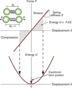
Figure 4.19 Atoms in crystals and glasses are linked by atomic bonds that behave like springs. The bond stiffness is S = F/δ. Stretching or compressing the bond by a displacement δ stores energy U = Fδ/2. The equilibrium (no force) atom separation is at the bottom of the energy well.

and this is the same in compression as in tension.
Table 4.1 lists the stiffnesses of the different bond types; these stiffnesses largely determine the value of the modulus, E. The covalent bond is particularly stiff (S = 20–200 N/m); diamond has a very high modulus because the carbon atom is small (giving a high bond density) and its atoms are linked by very strong springs (S = 200 N/m). The metallic bond is a little less stiff (S = 15–100 N/m) and metal atoms are often close packed, giving them high moduli too, though not as high as that of diamond. Ionic bonds, found in many ceramics, have stiffnesses comparable with those of metals, giving them high moduli too. Polymers contain both strong diamond-like covalent bonds along the polymer chain and weak hydrogen or Van der Waals bonds (S = 0.5–2 N/m) between the chains; it is the weak bonds that stretch when the polymer is deformed, giving them low moduli.
| Bond type | Examples | Bond stiffness, S (N/m) | Young’s modulus, E (GPa) |
|---|---|---|---|
| Covalent | Carbon–carbon bond | 50–180 | 200–1000 |
| Metallic | All metals | 15–75 | 60–300 |
| Ionic | Sodium chloride | 8–24 | 32–96 |
| Hydrogen bond | Polyethylene | 3–6 | 2–12 |
| Van der Waals | Waxes | 0.5–1 | 1–4 |
How is the modulus related to the bond stiffness? When a force F is applied to a pair of atoms, they stretch apart by δ. A force F applied to an atom of diameter ao corresponds to a stress ![]() , assuming each atom occupies a cube of side ao. A stretch of δ between two atoms separated by a distance ao corresponds to a strain ε = δ/ao. Substituting these into equation (4.15) gives
, assuming each atom occupies a cube of side ao. A stretch of δ between two atoms separated by a distance ao corresponds to a strain ε = δ/ao. Substituting these into equation (4.15) gives

Comparing this with equation (4.6) reveals that Young’s modulus, E, is approximately

The largest atoms (ao = 4 × 10⁻¹⁰ m) bonded with the weakest bonds (S = 0.5 N/m) will have a modulus of roughly
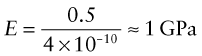
This is the lower limit for true solids. Many polymers have moduli of about this value. Metals and ceramics have values 50 to 1000 times larger because, as Table 4.1 shows, their bonds are stiffer. But as the E–ρ chart shows, materials exist that have moduli that are much lower than this limit. They are either foams or elastomers. Foams have low moduli because the cell walls bend easily (allowing large displacements) when the material is loaded. The origin of the moduli of elastomers takes a little more explaining.
The elastic moduli of elastomers
Think of it this way. An elastomer is a tangle of long-chain molecules with occasional cross-links, as on the left of Figure 4.20. The bonds between the molecules, apart from the cross-links, are weak—so weak that, at room temperature, they have melted. We describe this by saying that the glass temperature Tg of the elastomer—the temperature at which these weak bonds start to melt—is below room temperature. Segments are free to slide over each other, and were it not for the cross-links, the material would have no stiffness at all; it would be a viscous liquid.
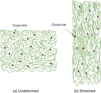
Figure 4.20 The stretching of an elastomer. Here the structure has been stretched to twice its original length. The stretching causes alignment, producing crystal-like regions. Thermal vibration drives the structure back to the one on the left, restoring its shape.
Temperature favors randomness. That is why crystals melt into disordered fluids at their melting point and evaporate into even more random gases at the boiling point. The tangle of Figure 4.20(a) has high randomness or, expressed in the terms of thermodynamics, its entropy is high. Stretching it, as on the right of the figure, aligns the molecules—some parts of it now begin to resemble the crystallites of Figure 4.18(b). Crystals are ordered, the opposite of randomness; their entropy is low. The effect of temperature is to try to restore disorder, making the material revert to a random tangle, and the cross-links give it a ‘memory’ of the disordered shape it had to start with. So there is a resistance to stretching—a stiffness—that has nothing to do with bond stretching, but with strain-induced ordering. A full theory is complicated—it involves the statistical mechanics of long-chain tangles—so it is not easy to calculate the value of the modulus. The main thing to know is that the moduli of elastomers are low because they have this strange origin and that they increase with temperature (because of the increasing tendency to randomness), whereas those of true solids decrease (because of thermal expansion).
Mixtures of atoms
Most engineering materials are not pure but contain two or more different elements. Often they dissolve in each other, like sugar in tea, but as the material is solid we call it a solid solution—examples are brass (a solution of zinc in copper), solder (a solution of tin in lead) and stainless steel (a solution of nickel and chromium in iron).
As we shall see later, some material properties are changed a great deal by making solid solutions. Modulus and density are not. As a general rule the density ![]() of a solid solution lies between the densities ρA and ρB of the materials that make it up, following a rule of mixtures (an arithmetic mean, weighted by volume fraction) known, in this instance, as Vegard’s law:
of a solid solution lies between the densities ρA and ρB of the materials that make it up, following a rule of mixtures (an arithmetic mean, weighted by volume fraction) known, in this instance, as Vegard’s law:
where f is the fraction of A atoms. Modulus is a bit more complicated—pure materials have only one kind of bond, A—A say; mixtures of A and B atoms have three: A—A, B—B and A—B. Within each bond type of Table 4.1 the stiffness ranges are not large, so mixtures of bonds again average out to values between those of the pure elements.
Alloying is not therefore a route to manipulating the modulus and density very much. To do this, mixtures must be made at a more macroscopic scale to make a hybrid material. We can mix two discrete solids together to make composites, or we can mix in some space to make foams. The effects on modulus and density are illustrated via the property chart in the next section.
4.5 Manipulating the modulus and density
Composites
Composites are made by embedding fibres or particles in a continuous matrix of a polymer (polymer matrix composites, PMCs), a metal (MMCs) or a ceramic (CMCs), as in Figure 4.21. The development of high-performance composites is one of the great material developments of the last 40 years, now reaching maturity. Composites have high stiffness and strength per unit weight, and—in the case of MMCs and CMCs—high-temperature performance. Here, then, we are interested in stiffness and weight.
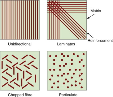
Figure 4.21 Manipulating the modulus by making composites, mixing stiff fibres or particles into a less-stiff matrix.
When a volume fraction f of a reinforcement r (density ρr) is mixed with a volume fraction (1 − f) of a matrix m (density ρm) to form a composite with no residual porosity, the composite density ![]() is given exactly by the rule of mixtures:
is given exactly by the rule of mixtures:
The geometry or shape of the reinforcement does not matter except in determining the maximum packing fraction of reinforcement and thus the upper limit for f (typically 50%).
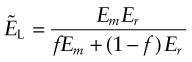
The modulus of a composite is bracketed by two bounds—limits between which the modulus must lie. The upper bound, ![]() , is found by assuming that, on loading, the two components strain by the same amount, like springs in parallel. The stress is then the average of the stresses in the matrix and the stiffer reinforcement, giving, once more, a rule of mixtures:
, is found by assuming that, on loading, the two components strain by the same amount, like springs in parallel. The stress is then the average of the stresses in the matrix and the stiffer reinforcement, giving, once more, a rule of mixtures:
where Er is the Young’s modulus of the reinforcement and Em that of the matrix. To calculate the lower bound, ![]() , we assume that the two components carry the same stress, like springs in series. The strain is the average of the local strains and the composite modulus is
, we assume that the two components carry the same stress, like springs in series. The strain is the average of the local strains and the composite modulus is
Example 4.4
A composite material has a matrix of polypropylene and contains 10% glass reinforcement. Estimate the Young’s modulus and density of the composite: (i) if the glass is in the form of long parallel fibres (calculate the properties parallel to the fibres); (ii) if the glass is in the form of small particles. Compare the specific moduli (E/ρ) of the constituent materials and the two composites and plot the four materials on a copy of Figure 4.22.
Use the following property data:
| E (GPa) | ρ (Mg/m3) | E/ρ | |
|---|---|---|---|
| Polypropylene (m) | 1 | 0.9 | 1.1 |
| Glass (r) | 70 | 2.2 | 31.8 |
Answer. The density of both composites is the same. Using (4.20) with f = 0.1 gives ![]() Mg/m3 (it would just sink in water). Using equation (4.21), Young’s modulus of the fibre-reinforced composite (parallel to the fibres) is
Mg/m3 (it would just sink in water). Using equation (4.21), Young’s modulus of the fibre-reinforced composite (parallel to the fibres) is ![]() GPa, with a specific modulus of
GPa, with a specific modulus of ![]() . Using equation (4.22), the modulus of the particle-reinforced composite would be
. Using equation (4.22), the modulus of the particle-reinforced composite would be ![]() , with a specific modulus
, with a specific modulus ![]() . The specific modulus of the fibre-reinforced composite is seven times that of the matrix, which is an enormous benefit if you want to build a low mass component or structure. That of the particle-reinforced composite is marginally lower than that of the matrix alone.
. The specific modulus of the fibre-reinforced composite is seven times that of the matrix, which is an enormous benefit if you want to build a low mass component or structure. That of the particle-reinforced composite is marginally lower than that of the matrix alone.
Figure 4.22 shows the range of composite properties that could, in principle, be obtained by mixing two materials together—the boundaries are calculated from equations (4.20)–(4.22). Composites can therefore fill in some of the otherwise empty spaces on the E–ρ chart, opening up new possibilities in design. There are practical limits of course—the matrix and reinforcement must be chemically compatible and available in the right form, and processing the mixture must be achievable at a sensible cost. Fibre-reinforced polymers are well-established examples—Figure 4.6 shows GFRP and CFRP, sitting in the composites bubble between the polymers bubble and the ceramics bubble. They are as stiff as metals, but lighter.
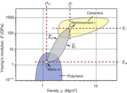
Figure 4.22 Composites made from a matrix m with a reinforcement r have moduli and densities, depending on the volume fraction and form of the reinforcement, that lie within the gray shaded lozenge bracketed by equations (4.21) and (4.22). Here the matrix is a polymer and the reinforcement a ceramic, but the same argument holds for any combination.
Foams
Foams are made much as you make bread: by mixing a matrix material (the dough) with a foaming agent (the yeast), and controlling what then happens in such a way as to trap the bubbles. Polymer foams are familiar as insulation and flotation and as the filler in cushions and packaging. You can, however, make foams from other materials: metals, ceramics and even glass. They are light for the obvious reason that they are, typically, 90% space, and they have low moduli. This might make them sound as though they are of little use, but that is mistaken: if you want to cushion or to protect a delicate object (such as yourself) what you need is a material with a low, controlled, stiffness and strength. Foams provide it.
Figure 4.23 shows an idealised cell of a low-density foam. It consists of solid cell walls or edges surrounding a void containing a gas. Cellular solids are characterised by their relative density, the fraction of the foam occupied by the solid. For the structure shown here (with t ≪ L) it is
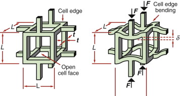
Figure 4.23 Manipulating the modulus by making a foam—a lattice of material with cell edges that bend when the foam is loaded.
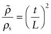
where ![]() is the density of the foam, ρs is the density of the solid of which it is made, L is the cell size and t is the thickness of the cell edges.
is the density of the foam, ρs is the density of the solid of which it is made, L is the cell size and t is the thickness of the cell edges.
When the foam is loaded, the cell walls bend, as shown on the right of the figure. This behavior can be modeled (we will be able to do so by the end of the next chapter), giving the foam modulus ![]()
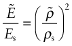
where Es is the modulus of the solid from which the foam is made. This gives us a second way of manipulating the modulus, in this case, decreasing it. At a relative density of 0.1 (meaning that 90% of the material is empty space), the modulus of the foam is only 1% of that of the material in the cell wall, as sketched in Figure 4.24. The range of modulus and density for real foams is illustrated in the chart of Figure 4.6—as expected, they fall below and to the left of the polymers of which they are made.
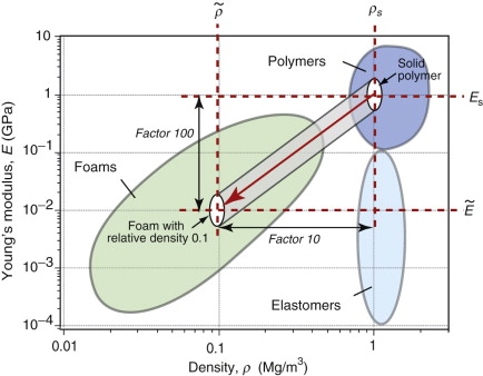
Figure 4.24 Foaming creates new materials with lower modulus and density. Low modulus is good for making packaging and protective shielding; low density is good for lightweight design and for flotation. The red arrow is a plot of equation (4.24).
4.6 Summary and conclusions
When a solid is loaded, it initially deforms elastically. ‘Elastic’ means that, when the load is removed, the solid springs back to its original shape. The material property that measures stiffness is the elastic modulus—and because solids can be loaded in different ways, we need three of them:
- Young’s modulus, E, measuring resistance to stretching.
- Shear modulus, G, measuring resistance to twisting.
- Bulk modulus, K, measuring the resistance to hydrostatic compression.
Many applications require stiffness at low weight, particularly ground, air and space vehicles, and that means a high modulus and a low density.
The density of a material is the weight of its atoms divided by the volume they occupy. Atoms do not differ much in volume, but they differ a great deal in weight. Thus, the density is principally set by the atomic weight; the further down the periodic table we go the greater becomes the density.
The moduli have their origins in the stiffness of the bonds between atoms in a solid and in the number of atoms (and thus bonds) per unit volume. The atomic volume, as we have said, does not vary much from one solid to another, so the moduli mainly reflect the stiffness of the bonds. Bonding can take several forms, depending on how the electrons of the atoms interact. The metallic, covalent and ionic bonds are generally stiff, hydrogen and Van der Waals bonds are much less so—that is why steel has high moduli and polyethylene has low.
There is very little that can be done to change the bond stiffness or atomic weight of a solid, so at first sight we are stuck with the moduli and densities of the materials we already have. But there are two ways to manipulate them: by mixing two materials to make composites, or by mixing a material with space to make foams. Both are powerful ways of creating ‘new’ materials that occupy regions of the E–ρ map that were previously empty.
Ashby M.F., Jones D.R.H. Engineering Materials 1 3rd ed 2006 Elsevier Butterworth-Heinemann Oxford, UK ISBN 0-7506-6380-4. (One of a pair of introductory texts dealing with the engineering properties and processing of materials.)
Askeland D.R., Phule P.P. The Science of Engineering Materials 5th ed 2006 Thompson Publishing Toronto, Canada (A mature text dealing with the science of materials, and taking a science-led rather than a design-led approach.)
Callister W.D. Materials Science and Engineering, An Introduction Jr 7th ed 2007 Wiley New York, USA ISBN 0-471-73696-1. (A long established and highly respected introduction to materials, taking the science-based approach.)
4.8 Exercises
- Exercise E4.1 Identify which of the five modes of loading (Figure 4.2) is dominant in the following components:
Can you think of another example for each mode of loading?
- Exercise E4.2 The cable of a hoist has a cross-section of 80 mm2. The hoist is used to lift a crate weighing 500 kg. What is the stress in the cable? The free length of the cable is 3 m. How much will it extend if it is made of steel (modulus 200 GPa)? How much if it is made of polypropylene, PP (modulus 1.2 GPa)?
- Exercise E4.3 Water has a density of 1000 kg/m3. What is the hydrostatic pressure at a depth of 100 m?
- Exercise E4.4 A catapult has two rubber arms, each with a square cross-section with a width 4 mm and length 300 mm. In use its arms are stretched to three times their original length before release. Assume the modulus of rubber is 10−3 GPa and that it does not change when the rubber is stretched. How much energy is stored in the catapult just before release?
- Exercise E4.5 Use the modulus–density chart of Figure 4.6 to find, from among the materials that appear on it:
- Exercise E4.6 Use the modulus–relative cost chart of Figure 4.7 to find, from among the materials that appear on it:
- Exercise E4.7 What is meant by:
- Exercise E4.8 The stiffness S of an atomic bond in a particular material is 50 N/m and its center-to-center atom spacing is 0.3 nm. What, approximately, is its elastic modulus?
- Exercise E4.9 Derive the upper and lower bounds for the modulus of a composite quoted as in equations (4.21) and (4.22) of the text. To derive the first, assume that the matrix and reinforcement behave like two springs in parallel (so that each must strain by the same amount), each with a stiffness equal to its modulus E multiplied by its volume fraction, f. To derive the second, assume that the matrix and reinforcement behave like two springs in series (so that both are stressed by the same amount), again giving each a stiffness equal to its modulus E multiplied by its volume fraction, f.
- Exercise E4.10 A volume fraction f = 0.2 of silicon carbide (SiC) particles is combined with an aluminum matrix to make a metal matrix composite. The modulus and density of the two materials are listed in the table. The modulus of particle-reinforced composites lies very close to the lower bound, equation (4.22), discussed in the text. Calculate the density and approximate modulus of the composite. Is the specific modulus, E/ρ, of the composite greater than that of unreinforced aluminum? How much larger is the specific modulus if the same volume fraction of SiC in the form of continuous fibres is used instead? For continuous fibres the modulus lies very close to the upper bound, equation (4.21).
| Density (Mg/m3) | Modulus (GPa) | |
|---|---|---|
| Aluminum | 2.70 | 70 |
| Silicon carbide | 3.15 | 420 |
- Exercise E4.11 Read the modulus E for polypropylene (PP) from the E–ρ chart of Figure 4.6. Estimate the modulus of a PP foam with a relative density
 of 0.2.
4.9 Exploring design with CES (use Level 2, Materials, throughout)
- Exercise E4.12 Make an E–ρ chart using the CES software. Use a box selection to find three materials with densities between 1000 and 3000 kg/m3 and the highest possible modulus.
- Exercise E4.13 Data estimation. The modulus E is approximately proportional to the melting point Tm in Kelvin (because strong inter-atomic bonds give both stiffness and resistance to thermal disruption). Use CES to make an E–Tm chart for metals and estimate a line of slope 1 through the data for materials. Use this line to estimate the modulus of cobalt, given that it has a melting point of 1760 K.
- Exercise E4.14 Sanity checks for data. A text reports that nickel, with a melting point of 1720 K, has a modulus of 5500 GPa. Use the E–Tm correlation of the previous question to check the sanity of this claim. What would you expect it to be?
- Exercise E4.15 Explore the potential of PP–SiC (polypropylene–silicon carbide) fibre composites in the following way. Make a modulus–density (E–ρ) chart and change the axis ranges so that they span the range 1 < E < 1000 GPa and 500 < ρ < 5000 kg/m3. Find and label PP and SiC, then print it. Retrieve values for the modulus and density of PP and of SiC from the records for these materials (use the means of the ranges). Calculate the density
 and upper and lower bounds for the modulus
  at a volume fraction f of SiC of 0.5 and plot this information on the chart. Sketch by eye two arcs starting from (E, ρ) for PP, passing through each of the (
 ) points you have plotted and ending at the (E, ρ) point for SiC. PP–SiC composites can populate the area between the arcs roughly up to f = 0.5 because it is not possible to insert more than this.
 - Exercise E4.16 Explore the region that can be populated by making PP foams. Expand an E–ρ plot so that it spans the range 10−4 < E < 10 GPa and 10 < ρ < 2000 kg/m3. Find and label PP, then print the chart. Construct a band starting with the PP bubble by drawing lines corresponding to the scaling law for foam modulus
 (equation (4.24)) touching the top and the bottom of the PP bubble. The zone between these lines can be populated by PP foams.
4.10 Exploring the science with CES Elements
- Exercise E4.17 The text cited the following approximate relationships between the elastic constants Young’s modulus, E, the shear modulus, G, the bulk modulus, K and Poisson’s ratio, ν:
Use CES to make plots with the bit on the left-hand side of each equation on one axis and the bit on the right on the other. To do this you will need to use the Advanced facility in the dialog box for choosing the axes to create functions on the right of the two equations. How good an approximation are they?
- Exercise E4.18 The cohesive energy Hc is the energy that binds atoms together in a solid. Young’s modulus E measures the force needed to stretch the atomic bonds and the melting point, Tm, is a measure of the thermal energy needed to disrupt them. Both derive from the cohesion, so you might expect E and Tm to be related. Use CES to plot one against the other to see (use absolute melting point, not centigrade or fahrenheit).
- Exercise E4.19 The force required to stretch an atomic bond is
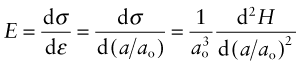
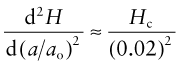
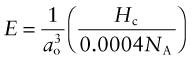
where dH is the change in energy of the bond when it is stretched by da. This force corresponds to a stress
The binding energy per atom in a crystal, Ha, is
where Hc is the cohesive energy and NA is Avogadro’s number (6.022 × 10²³/mol). If we assume that a stretch of 2% is enough to break the bond, we can make the approximation:
giving
Make a plot of Young’s modulus E against the quantity on the right of the equation (using the ‘Advanced’ facility in the dialog box for choosing the axes) to see how good this is. (You will need to multiply the right by 10−9 to convert it from pascals to GPa.)


1 Archimedes (287–212 BC), Greek mathematician, engineer, astronomer and philosopher, designer of war machines, the Archimedean screw for lifting water, evaluator of π (as 3 + 1/7) and conceiver, while taking a bath, of the principle that bears his name.
2 Isaac Newton (1642–1727), scientific genius and alchemist, formulator of the laws of motion, the inverse-square law of gravity (though there is some controversy about this), laws of optics, the differential calculus and much more.
3 Blaise Pascal (1623–1662), philosopher, mathematician and scientist, who took a certain pleasure in publishing his results without explaining how he reached them. Almost all, however, proved to be correct.
4 Robert Hooke (1635–1703), able but miserable man, inventor of the microscope, and perhaps, too, of the idea of the inverse-square law of gravity. He didn’t get along with Newton.
5 Thomas Young (1773–1829), English scientist, expert on optics and deciphering ancient Egyptian hieroglyphs (among them, the Rosetta stone). It seems a little unfair that the modulus carries his name, not that of Hooke.
6 Siméon Denis Poisson (1781–1840), French mathematician, known both for his constant and his distribution. He was famously uncoordinated, failed geometry at university because he could not draw, and had to abandon experimentation because of the disasters resulting from his clumsiness.
7 Very low density foams and gels (which can be thought of as molecular-scale, fluid-filled, foams) can have lower moduli than this. As an example, gelatine (as in Jell-O) has a modulus of about 10−5 GPa.