6 HDRI – Increasing Dynamic Range

In spite of rapid improvements that have been made in camera technology in recent years, we still often come across scenes which encompass a broader tonal range than a normal digital camera is capable of capturing. Shooting multiple images with different exposure settings and then merging those images into one allows the photographer to create images with extended dynamic range. This technique produces what are known as HDRIs, or High Dynamic Range Images. The acronym DRI stands for “Dynamic Range Increase”. Here, the term “dynamic range” describes the difference in brightness between the pixels with the brightest and the darkest tonal values within an image.
You can also reduce image noise by merging several images of the same scene which have been exposed slightly differently and averaging the pixel values of the individual images in the sequences. This enables photographers to shoot in low-light situations using high ISO speeds and short shutter speeds without having to accept the image noise which such circumstances normally produce. We will describe both of these techniques in this chapter.
To increase dynamic range, we will be using Photoshop, PhotoAcute, Photomatix Pro, and FDRTools. For the noise reduction section, we will be using just PhotoAcute. Simple overlay effects are most easily achieved using Photoshop. A typical HDR workflow consists of five phases:
1. Shooting phase – creation of the source images
2. Merging – i.e., the actual production of the HDRI image
3. Optional optimization of the HDR image
4. Tone mapping – reducing the dynamic range to a spectrum that can be displayed on normal monitors and easily printed
5. Post-processing (fine-tuning)
6.1 High Dynamic Range Images and Tone Mapping
![]() A relatively simple introduction to HDR Imaging can be found at www.hdrsoft.com/resources/dri.html. Part of the information presented here originates from that web site. Christian Bloch has written a great book on the subject, and Jack Howard’s “Practical HDRI” [5] is also a useful source of information.
A relatively simple introduction to HDR Imaging can be found at www.hdrsoft.com/resources/dri.html. Part of the information presented here originates from that web site. Christian Bloch has written a great book on the subject, and Jack Howard’s “Practical HDRI” [5] is also a useful source of information.
Due to the limitations of technical light-capturing processes, neither film nor digital cameras can always adequately capture the entire tonal range of a high-contrast scene. The dynamic range (i.e., the difference between the brightest and darkest parts) of a scene is often simply too great. Black-and-white or color negative film is capable of differentiating and reproducing contrast of about 4,000:1. This represents an exposure range of between 10 and 12 f-stops (12 in the case of black-and-white negative film). Color slide material can generally differentiate a range of about 7 to 8 f-stops. The differentiation potential of a good DSLR lies somewhere between only 8 to 10.5 f-stops, with the higher values being achieved by the newest camera models with larger image sensors. Some FujiFilm cameras use so-called Super CCD sensors, which attempt to improve dynamic range by utilizing two sensor elements per pixel – one element for bright and mid-range tones, and a larger, separate element for recording darker tones.
The image sensors in digital cameras also tend to lose sensitivity more rapidly at the top and bottom of the exposure range than film material, as depicted in Figure 6-1.
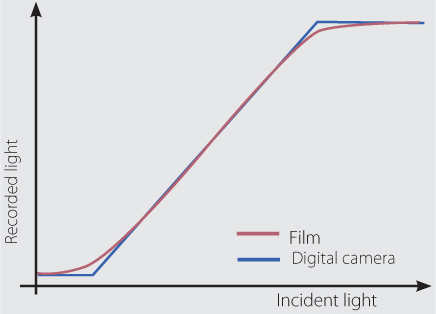
Figure 6-1: Light sensitivity curves for film and digital camera image sensors.
In a high-contrast scene – in broad daylight, for example – the range of contrast can be as much as 100,000:1.* The photographer usually only has the choice between exposing for the mid-range, for shadows, or for the highlights present in a scene. Figure 6-2 illustrates just such a situation.
Ideally, we want to reproduce as much of this range as possible in the digital original as well as in any prints we may make. The human eye can adapt to different lighting situations much more quickly and easily than a camera – a single glance can accommodate light within a range of about 100,000:1 (or 105:1). Given a little time to adjust, this increases to 1012:1. The human eye is capable of seeing and registering starlight with a strength of 0.000.001 cd/m2 just as well as bright sunlight with a strength of 1,000,000 cd/m2. This is equivalent to a range of 32 f-stops.
Image sensor technology is constantly improving and modern cameras can capture significant dynamic range – even if the progress from camera generation to generation is sometimes agonizingly slow. There is, however, already another option, which involves taking multiple exposures of a scene using differing exposure settings, and then merging the resulting images into a single, high dynamic range image. This is the basic HDR image concept. “Normal” images (with less or standard dynamic range) are described as LDR (Low Dynamic Range). HDRI is a technique which has long been used in the digital video sphere, but which has only been introduced into digital still photography fairly recently. HDR functionality first appeared in the CS2 version of Photoshop, and was improved greatly in the CS3 version by the introduction of more 32-bit data support.
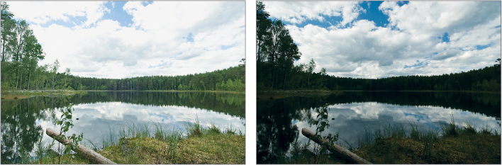
Figure 6-2: A typical, somewhat contrast rich scene. The image to the left was exposed so the shadows display texture. The image to the right was exposed so the highlights display texture (i.e., in the sky).
![]() Normal images – those with standard or low dynamic range – are called “Low Dynamic Range Images” (LDRI or LDR images). The term MDR (standing for “Medium Dynamic Range”) is also sometimes used.
Normal images – those with standard or low dynamic range – are called “Low Dynamic Range Images” (LDRI or LDR images). The term MDR (standing for “Medium Dynamic Range”) is also sometimes used.
In order to be able to truly differentiate the tonal values in a digital image with substantial dynamic range, it is necessary to maximize the precision of the tonal values of each individual pixel, which in turn, requires a great deal of memory space. Limited dynamic range can be captured and displayed using 8-bits per pixel and color channel. RAW images generally have 12 or 14 effective bits per pixel when they are downloaded from a camera (even if they are saved as 16-bit images) and show noticeably greater dynamic range.
If you want to further increase dynamic range and the ability to differentiate between tonal values, you will need to resort to even higher values of 32 bits per pixel and color channel. Theoretically, this will enable you to encompass a range equivalent to 32 f-stops. 16- or 32-bit images, however, are not automatically HDR images, although the potential dynamic range they possess is one of the prerequisites for producing effective HDR results. This type of image processing requires the use of special 32-bit file formats such as OpenEXR or 32-bit TIFF.* Photoshop can also save HDR images in PSD or PSB formats, as well as PBM (Portable Bit Map) or Radiance file formats. Nowadays, there is a whole range of different HDR formats available, each with its own advantages and disadvantages.
![]() 16-bit drivers and printing plug-ins have only been available since about 2007, and are still not available for all printers and operating systems. They improve color rendering, but cannot increase dynamic range.
16-bit drivers and printing plug-ins have only been available since about 2007, and are still not available for all printers and operating systems. They improve color rendering, but cannot increase dynamic range.
While HDR image creation is a subject in its own right, the reproduction of HDR images is another matter entirely. Most typical output media – monitors, offset printing, or inkjet printing – are not capable of reproducing the dynamic range of HDR images satisfactorily. Modern printing techniques are generally limited to 8-data bits per RGB or CMYK color channel, and often raise the question of whether even the resulting 256 color values can be genuinely and faithfully reproduced using the currently available technology. Generally speaking, printed output will display closer to 120–180 different tonal values.
The solution to this problem lies in effective compression and display of tonal values, known as tone mapping. The goal of tone mapping is to reduce the large amounts of image tonal value data available in a high dynamic range image into a range that can be reproduced conventionally while retaining the attractive look of the original HDR image. This is generally only possible within a limited range using linear regression techniques. During tone mapping processes, it very important to differentiate between pixels with high, mid, or shadow values and to see these in relation to their neighboring pixels as well as within the context of the entire image.
Unfortunately there isn’t a single tone mapping method which works equally well for all images, and this makes automatic tone mapping techniques difficult to realize. As a result, most of the tone mapping methods presented here will involve hands-on user involvement, and you will need to experiment to develop your own methodology and feel for how best to process your own images.
6.2 Shooting Techniques for HDR Images
HDR images are constructed from a number of individual exposures shot with differing exposure values. This is generally quite easy for non-moving subjects, but is more difficult to achieve for scenes that contain moving objects. Here are the main points to keep in mind when shooting HDR sequences:
▸ A stable tripod is essential, even though most HDR modules enable users to also merge images that are not perfectly matched using a stitching-type process. This type of process nevertheless reduces precision and increases the risk of losing edge detail due to cropping.
▸ In order to maintain uniform depth of field, you should only vary the shutter speed, and not the aperture. Use the Av (or A) exposure mode setting (see figure 6-3).
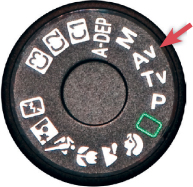
Figure 6-3: Use the Av or A (Aperture Priority) or manual exposure mode when shooting for HDR images.
▸ In order to avoid differences in depth of field, switch the camera to manual focus. This will ensure that the camera’s autofocus system does not refocus between shots.
▸ To avoid ghosting effects in your HDR images, avoid shooting moving objects, such as the pedestrians shown in figure 6-4.
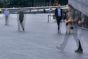
Figure 6-4: If moving objects are present in a scene, ghosting may result.
▸ If you are prepared to limit yourself to three exposures, then the auto-bracketing function available on most DSLRs (set to aperture priority –Av) is a good choice. If, however, you wish to obtain maximum dynamic range in high-contrast scenes, you will probably have to add additional manual shots to your sequence. Many cameras only allow for three bracketed shots.
If you use a bracketing increment of 2 EVs (in this case shutter speed values varied by a factor of 4) per shot, then three exposures allow for a maximum dynamic range of 4 f-stops plus the basic 8–10 f-stops your camera can capture in a single shot. The bracketing settings can be found in most DSLRs in the AEB (Auto Exposure Bracketing) menu (see figure 6-5). The exact sub-menu structure will vary, depending on your camera model. The maximum number of bracketed shots and the maximum bracketing interval will depend on the capabilities of your camera. Some cameras can shoot bracketing sequences of more than three exposures. These include the Nikon D200 and D300, as well as the Canon EOS DS1 Mark III. If you need more bracketed shots than your camera allows, you will have to program multiple bracketing sequences with differing shutter speed settings. Keep in mind, however, that not every high-contrast scene needs to be captured with the same extremes of tonal value range.
▸ The necessary practical steps are as follows: Use your camera’s spot metering mode to meter the darkest shadows in your scene and record the values. Then repeat the process for mid-tones and highlights. You can then use the two extreme values to calculate the number of f-stops you need to cover, and thus the number of shots you need to include in your sequence.
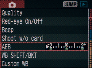
Figure 6-5: The bracketing settings in a Canon 20D – to be found in the AEB menu.
If you want to capture the entire tonal range of a scene, you need to make sure the brightest image doesn’t have any washed-out highlights and that the darkest image doesn’t have any underexposed shadows. Washed-out highlights are easily recognized using a DSLR’s image preview function, and the histograms displayed by most modern cameras will help you to locate underexposed image areas.* The histogram of the brightest image should not show values at the extreme left of the graph (in the shadows), and the graph for the darkest image should not have significant values at the right hand end of the scale (highlights). The most reliable way to check exposure is using an RGB histogram (see figure 6-6), which shows the tonal values for the individual color channels in your image. A luminance histogram evaluates the individual color channels at different strengths (green is displayed the strongest), which can make it difficult to recognize the true impact of the red or blue channels. While washed-out highlights are generally not acceptable in an image, underexposed shadows can sometimes be considered part of an effective composition, especially in night shots or other low-key situations which include very dark image elements.

Figure 6-6: To capture the entire dynamic range in a scene, the darkest image shouldn’t contain any tonal values equivalent to the highlights (right) and the brightest image shouldn’t contain shadows (left). The center image can contain some overlap (These are Lightroom histograms).
▸ If you are shooting in JPEG or TIFF formats, you should always use the same white balance settings. RAW images should all be converted using the same color temperature setting for white balance. If your camera calculates and embeds differing white balance values in your image files, you will have to transfer the settings from your reference image to all the other images in your sequence during the conversion process.*
▸ Disable your camera’s “Auto ISO” setting (if available), and select a suitable preset ISO value.
6.3 Simple Photoshop Blending Techniques
Combining Two Differently Exposed Shots
Occasionally, you may have two or more shots that are nearly identical, but where each image contains areas which are better or more pleasingly exposed than the equivalent areas in the other image. Instead of using a classic HDRI program to process these images, it’s often easier and faster to merge them in Photoshop using the Layers command and layer masks to blend the appropriate areas. There are a number of different ways of going about this, and we will describe two of the possible techniques.
We have two source images (figures 6-7 and 6-8). The shell in the first image (6-7) is pleasingly lit with diffuse light from above. However, that same light casts a hard shadow on the sea urchin below the shell. In the second image (figure 6-8), the sea urchin is better lit, but the shell is not as bright. These two images can be blended together using a simple and effective technique.
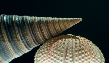
Figure 6-7: In this shot, the shell is pleasingly lit, but casts a hard shadow.
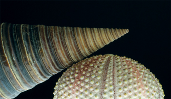
Figure 6-8: In this shot the sea urchin is well illuminated, but the shell is poorly defined.
To get started, open both images in Photoshop and drag the image in figure 6-7 over the one in figure 6-8 while holding down the ![]() key.** Select the upper layer using the Layers palette and reduce its opacity until you are able to see whether the two images are correctly aligned. If not, use the move tool
key.** Select the upper layer using the Layers palette and reduce its opacity until you are able to see whether the two images are correctly aligned. If not, use the move tool ![]() to shift the upper image so that it coincides exactly with the lower one. It may also be necessary to rotate the image slightly. Once this is done, we set the opacity of the upper image back to 100%.
to shift the upper image so that it coincides exactly with the lower one. It may also be necessary to rotate the image slightly. Once this is done, we set the opacity of the upper image back to 100%.
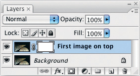
Figure 6-9: The Layers palette after our first blending attempt.
If you are using Photoshop CS4, you can replace this entire process by loading your images using File ▸ Scripts ▸ Load Files into Stack. Simply select both layers and use Edit ▸ Auto-Align Layers with the Collage layout setting to align your images.
Next, we create a white (empty) layer mask for the active upper layer (click on ![]() at the bottom of the Layers palette). Remember to explicitly select the layer mask using a single click on the mask icon in the Layers palette entry. Our Layers palette now looks like the one shown in figure 6-9.
at the bottom of the Layers palette). Remember to explicitly select the layer mask using a single click on the mask icon in the Layers palette entry. Our Layers palette now looks like the one shown in figure 6-9.
We then use a large, soft brush (hardness 5–10%) to paint black into those areas of the mask where the lower layer should show through. We recommend using a brush opacity of 15–25% and repainting the same area multiple times if necessary. This will give you more control over the exact structure of your mask. In the places where the mask is black, Photoshop will display the layer below. In those areas where it is white, only the upper layer will be visible. The gray areas are partially transparent, based on the corresponding darkness of the area in question.
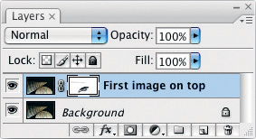
Figure 6-10: The Layers palette after creating the Layer Mask for the blending process.
After a couple of brush strokes with the black brush, the corresponding parts of the lower layer will become visible in the black-painted areas. During this whole process, it is very important to make sure that the shadows and highlights not being manipulated remain natural-looking. This is why we also darkened the upper edge of the shell slightly with a gray brush stroke (which is, in fact, a low opacity black brush stroke).
The result can be seen in figure 6-11. Figure 6-12 show the corresponding layer mask, and figure 6-10 shows the layer stack with the mask icon on the upper layer.
We could also have created a similar transparency effect by working directly in the upper image using the Eraser tool ![]() . Working with a layer mask, however, allows you to undo any mistakes you might make by repainting the mask, or erasing the sections of the mask that don’t suit your purposes.
. Working with a layer mask, however, allows you to undo any mistakes you might make by repainting the mask, or erasing the sections of the mask that don’t suit your purposes.
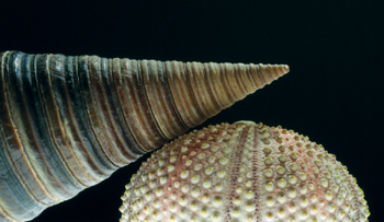
Figure 6-11: The blended image made from two layers, and using a blending mask in the upper layer.
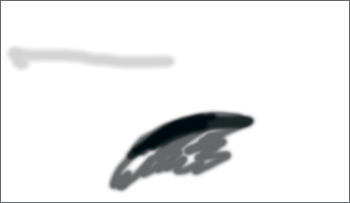
Figure 6-12: The Layer Mask used for the blending process. The mask is linked to the upper image layer, making the black areas transparent.
Replacing a Traditional Gradation Filter
Landscape photographers often cannot get by without using a neutral gray gradation filter. In the days of black-and-white photography, such a filter (or a red filter) was practically a must. A gradation filter can often be used to darken a bright sky at the shooting stage, while retaining a smooth transition between the sky and the horizon. However, filters and filter mounts can be tricky to align and are bulky to carry around. These types of filters can still be useful to a digital photographer, but if you don’t have one with you, you can simulate the same effect digitally. Simply take multiple shots of your scene using shutter speed bracketing. You can then blend two images together – one with the sky exposed correctly, and the other with the landscape itself exposed correctly. This process is called Exposure Blending.*
Figures 6-13 and 6-14 show our two source images (after conversion to black-and-white). The image on the left was exposed to show the detail in the landscape portion of the image, resulting in a flat-looking sky. The image on the right was exposed using a shutter speed that was 1½ stops faster, allowing the textures in the sky to come to the fore, and causing the landscape itself to be under-exposed. We will now merge these two images together to achieve a better overall result.
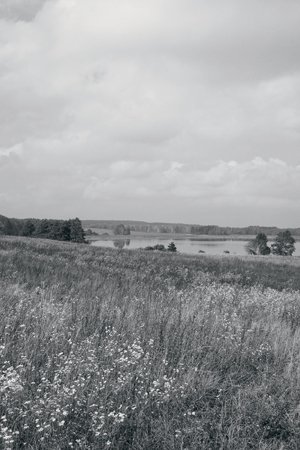
Figure 6-13: This shot was exposed to show the landscape detail.
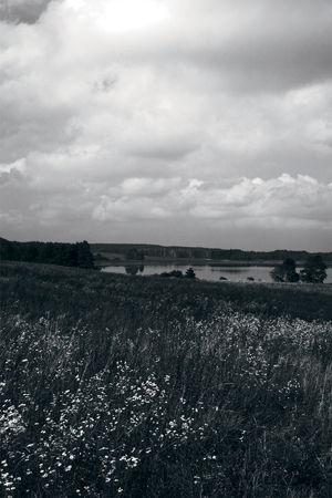
Figure 6-14: This shot was exposed to show detail in the sky.
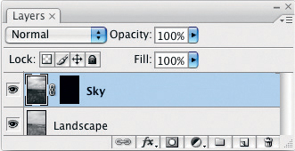
Figure 6-15: The “landscape” image is on the lower layer, and the “sky” image is on the upper layer.
We open and align our two images in Photoshop using the technique previously described (e.g., using the Load Files into Stack script). We now activate the upper layer (with the darker sky) and apply a black layer mask by clicking the ![]() symbol in the Layers palette while holding down the
symbol in the Layers palette while holding down the ![]() key (Mac:
key (Mac: ![]() key). Figure 6-15 shows the resulting Layers palette. Photoshop now displays our lower “landscape” image.
key). Figure 6-15 shows the resulting Layers palette. Photoshop now displays our lower “landscape” image.
In this case, we will be using the gradient tool ![]() instead of a brush tool to manipulate our image. The effect we want to achieve will mask the landscape in the upper layer and provide a gradual transition between the horizon and the sky.
instead of a brush tool to manipulate our image. The effect we want to achieve will mask the landscape in the upper layer and provide a gradual transition between the horizon and the sky.
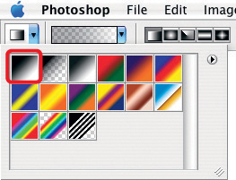
Figure 6-16: Select the top left gradient pattern.
We select a linear gradient from black to transparent in the activated ![]() tool (see Figure 6-16). If we then set the background color in the Photoshop toolbar to white, the gradient takes on a white to transparent progression.
tool (see Figure 6-16). If we then set the background color in the Photoshop toolbar to white, the gradient takes on a white to transparent progression.
We then point the mouse to the upper edge of the image (the “center point”) and drag it down to shortly above the horizon near the level of the lake (our “end point”). This causes our dramatic sky to become visible again, while creating a seamless transition between the horizon and the sky. The trees on the horizon have become a little darker, but still appear natural.
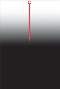
Figure 6-17: The layer mask created using the gradient tool. The red arrow indicates the direction in which we dragged the gradient.
Figure 6-17 shows the layer mask we created to fine-tune the transition between the horizon and the sky. This mask can be further manipulated and perfected using any number of Photoshop tools, but the standard gradient mask is sufficient for our purposes.
We enhanced our resulting image slightly using the DOP Detail Extractor (described in section 7.1). Here, we also used a layer mask to avoid increasing the local contrast in the sky. This mask was basically the opposite of our blending mask, and was also created using the gradient tool. Another option would have been to duplicate the existing layer mask and invert it using Image ▸ Adjust ▸ Invert (or ![]() ).
).
Finally, we sharpened our image slightly using the USM filter, also with the additional use of a mask to avoid unwanted sharpening of the sky – in this case, the same mask we used to protect the sky from local contrast enhancement.
To create a copy of a layer mask, go to the Layers palette, and then drag the mask you want to copy from one layer entry to another while holding down the ![]() key (on a Mac, use the
key (on a Mac, use the ![]() key).
key).
The Layers palette shown in figure 6-18 illustrates the various layers we used while processing this image, including all the post-processing corrections. Figure 6-19 shows the final image.
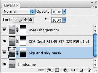
Figure 6-18: The Layers palette of the final, processed image. The top two layers are used to improve local contrast and sharpness.
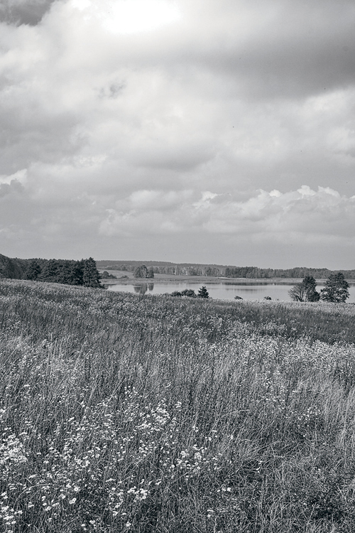
Figure 6-19: The final image consisting of the two blended layers and some slight microcontrast enhancement.
6.4 Creating HDR Images Using PhotoAcute
![]() The usual three HDRI phases (shooting, merging, tone mapping) are reduced to simply shooting and merging when using PhotoAcute. This simplifies the process but lessens user control over the tone mapping process.
The usual three HDRI phases (shooting, merging, tone mapping) are reduced to simply shooting and merging when using PhotoAcute. This simplifies the process but lessens user control over the tone mapping process.
The basic functions of PhotoAcute have already been addressed in section 3.3. One of the numerous functions the program offers is the creation of increased dynamic range images. In contrast to Photoshop’s Merge to HDR function (which we will describe in section 6.5), the PhotoAcute functions described below only work for 8- or 16-bit images.*
The possibilities for user control are relatively limited, as we’ve already learned in section 3.3. Nevertheless, the results produced in many simpler scenarios are quite acceptable, and are also quick and easy to realize.
Our choice of source formats (as previously described) includes JPEG, TIFF (8- or 16-bit), DNG files, or other RAW formats supported by the Adobe DNG converter.
As a rule, we recommend that you either do not preprocess your images at all, or that you limit yourself to any necessary white balance correction or cropping before saving your source images as 16-bit TIFF files. As always, make sure any preprocessing steps are applied in equal amounts to all of your source images.
For our example, we will load our non-preprocessed TIFF files into the PhotoAcute processing list using the program’s File ▸ Open function. We then inspect our images and select the ones we want to use. At this point, if we are going to use the Correct image geometry or Fix color fringing functions, we need to check that the program has correctly identified our camera and lens. If the camera or lens was incorrectly recognized, we reset the parameters manually using Settings ▸ Camera. If PhotoAcute does not yet support the lens you are using, you can either select a similar one from the menu, or simply switch off the corrections which are not supported (see figure 6-21).
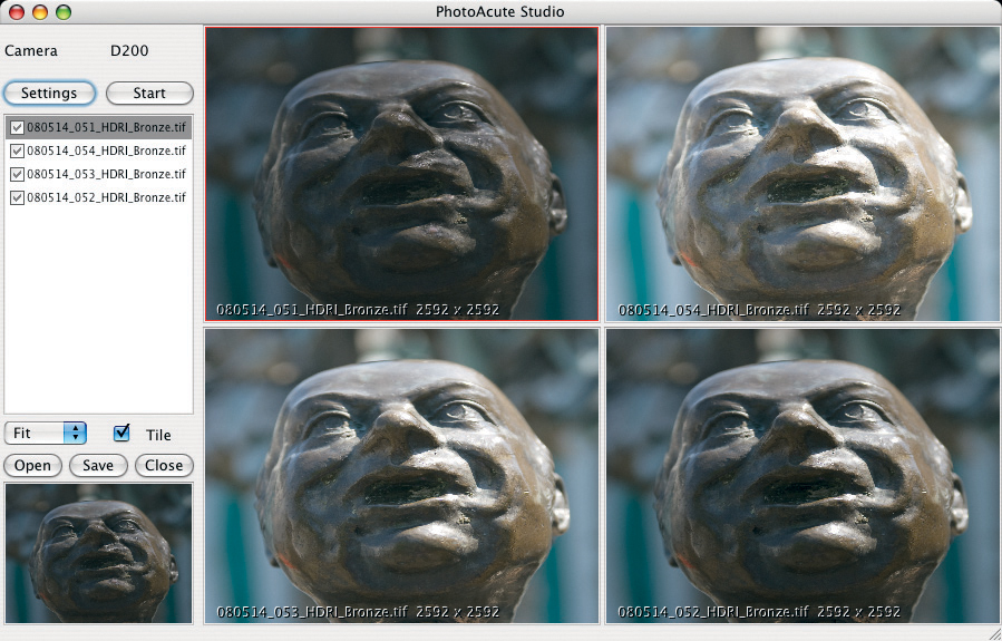
Figure 6-20: The PhotoAcute window after loading our source files. Don’t be misled by the sometimes extremely distorted images in this window. These are only previews images which have been adjusted to fit into the available window space.
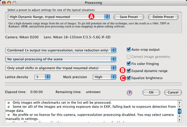
Figure 6-21: The PhotoAcute settings for DRI processing.
In order to create an image with extended dynamic range, we start by activating Expand dynamic range ![]() and Equalize brightness
and Equalize brightness ![]() (see figure 6-21), provided these haven’t already been automatically activated by a preset from menu
(see figure 6-21), provided these haven’t already been automatically activated by a preset from menu ![]() .
.
Because PhotoAcute DRI images generally require post-processing, we recommend using 16-bit source images and exporting to a 16-bit output format. This will only work if your source images are RAW or 16-bit TIFF files. JPEG source images can provide a maximum of 8-bit color depth.
For our example we will use the head of a bronze figure mounted on a decorative fountain. We started by cropping the head to a square format in our RAW converter (Photoshop Lightroom), and then exported the resulting five 16-bit TIFF images into PhotoAcute.
Our DRI processing settings can be seen in figure 6-21. Our Nikkor 28–70 mm f2.8 lens is not yet supported by PhotoAcute, so we set the program to a different (but similar) lens and switched off the Correct image geometry function.
Specific tone mapping settings are not part of the available options. We also activated the Expand dynamic range option ![]() , and we deactivated the Equalize brightness option
, and we deactivated the Equalize brightness option ![]() for the first run.
for the first run.
The result can be seen in figure 6-22 and, although not ideal, it is an improvement on the original, and was created without any extra tone mapping. The “grunge” look common to many HDR images is not visible in our example, which we consider to be a positive aspect of the result. The image is generally slightly dark, but this can be easily remedied using the Photoshop Shadows/Highlights tool.
As an experiment, we processed the same images a second time with similar settings, but this time with the Equalize brightness ![]() option activated. The result can be seen in figure 6-23. This image is visibly brighter, but this can also be corrected using Shadows/Highlights, this time to darken the highlights instead of lightening the shadows, as we did in our previous example.
option activated. The result can be seen in figure 6-23. This image is visibly brighter, but this can also be corrected using Shadows/Highlights, this time to darken the highlights instead of lightening the shadows, as we did in our previous example.
When working in PhotoAcute, keep in mind the role of the reference image you selected at the start of the process. This is the image which is highlighted blue in the selection list when you click the Start button. If you use a bright reference image, the resulting image will also be brighter. For darker results, select a darker reference image.
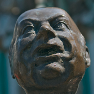
Figure 6-22: The result of our first PhotoAcute DRI run without the “Equalize brightness” option activated.
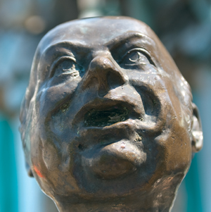
Figure 6-23: The result of our second run – this time with “Equalize brightness” activated.
As you can see, PhotoAcute’s DRI functionality is sparsely equipped, but delivers usable results quickly and easily for straightforward projects. If, however, you plan to post-process your HDR images using Photoshop, you will need to use a different program or save your processed image to the Radiance HDRI format (this option is only supported since version 2.8). You can then tone map your HDR image using either Photoshop, Photomatix Pro, or FDRTools.
6.5 Creating HDR Images Using Photoshop’s HDR Functionality
As previously mentioned, Photoshop has included HDR functionality since the CS2 version. This functionality was extended in the CS3 version to include more tone mapping methods, which we will describe later. CS3 and future versions are also becoming increasingly 32-bit capable, and support for 32-bit processing is already available in the Levels, Hue/Saturation, Channel Mixer, Photo Filter, and Exposure tools. (A number of Adobe’s HDRI options are only available in the “Extended” versions of Photoshop CS3 or CS4.)
We have already described the basics of HDRI shooting techniques. Figure 6-24 shows our new source images and their corresponding histograms. The brightest image shows no shadow clipping, and the darkest one shows no discernible highlight clipping. The shutter speeds were each about two stops apart.
To create an HDR image in Photoshop, navigate to File ▸ Automation ▸ Merge to HDR. Because it is almost impossible to avoid slight shifts in your source images – even when using a tripod – it is necessary to activate option ![]() Attempt to Automatically Align Source Images in the dialog box illustrated in figure 6-25. Deactivating this option can lead to ghosting effects. Now use the dialog shown in figure 6-25 to select the images you want to merge.
Attempt to Automatically Align Source Images in the dialog box illustrated in figure 6-25. Deactivating this option can lead to ghosting effects. Now use the dialog shown in figure 6-25 to select the images you want to merge.
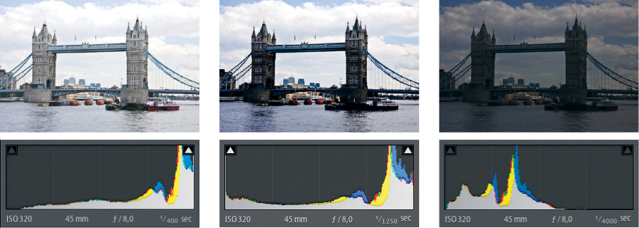
Figure 6-24: Our three source images and their corresponding Lightroom histograms.
You can perform these steps in Bridge by selecting Tools ▸ Photoshop ▸ Merge to HDR, or in Lightroom (version 2 and higher) using Merge Photos to HDR in Photoshop in the Edit menu. However, both these methods do not include the option of aligning the source images. As of Photoshop CS3, however, the alignment option is automatically activated, even for instances where the images have been opened using Lightroom or Bridge).
The “normal” Photoshop dialog (accessed via File ▸ Automation ▸ Merge to HDR) is shown in figure 6-25.
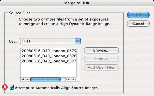
Figure 6-25: The dialog box used to select the source images for an HDR image. We recommend activating option ![]() .
.
Photoshop starts by loading the files, then aligns and merges them into a (temporary) HDR image. Additionally, it will generate a preview (see figure 6-26). This can use a lot of processing power, and may take some time (even using a faster computer). In the dialog displayed in figure 6-26, you can use the preview list ![]() to deactivate (exclude) selected images from the merge process.
to deactivate (exclude) selected images from the merge process.
The EVs which can be seen below each image thumbnail are either automatically extracted from each file’s EXIF data or estimated automatically by the program. The histogram ![]() shows the dynamic range of the merged image. Use the slider beneath this histogram to find an appropriate white point – in our experience, this will be further to the right than to the left end of the slider scale.
shows the dynamic range of the merged image. Use the slider beneath this histogram to find an appropriate white point – in our experience, this will be further to the right than to the left end of the slider scale.
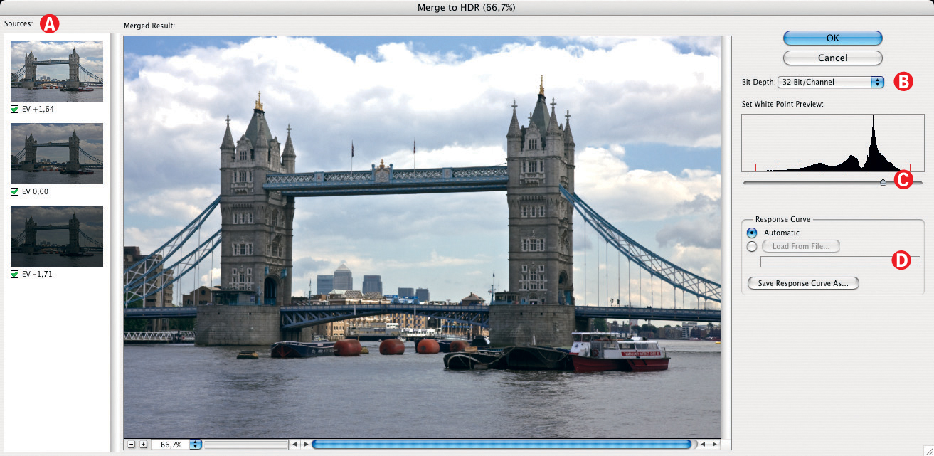
Figure 6-26: The preview of an HDR image in Photoshop CS3. To the upper right you can select the bit depth for the resulting image.
You can select the desired bit depth (8-, 16-, or 32-bit) for the resulting image using the dropdown menu ![]() . We suggest using 32-bit images for your first attempt. Click on OK and Photoshop will start the merging process and then display the resulting HDR image. Photoshop will give the file a “.pfm” extension, which stands for “Portable Floating Map”.*
. We suggest using 32-bit images for your first attempt. Click on OK and Photoshop will start the merging process and then display the resulting HDR image. Photoshop will give the file a “.pfm” extension, which stands for “Portable Floating Map”.*
Do not be irritated by the look of the preview image (the previews shown in figure 6-26 or 6-27 have a relatively normal appearance because the scene has a relatively moderate dynamic range). In the case of images with a much larger dynamic range, Photoshop has to create a temporarily tone mapped preview image which simply cannot be displayed on a conventional computer monitor.

Figure 6-27: A provisionally tone-mapped preview of our Photoshop HDR image.
You can now adjust the brightness of the image using the slider ![]() (at the bottom left in the preview image shown in figure 6-27). Adjusting this value does not, however, change your actual image. It is designed simply to enhance the preview image in order to help you to make good subsequent processing decisions.
(at the bottom left in the preview image shown in figure 6-27). Adjusting this value does not, however, change your actual image. It is designed simply to enhance the preview image in order to help you to make good subsequent processing decisions.
You can also make changes to the tone-mapping preview using the settings located at View ▸32-Bit Preview Options. This opens the dialog shown in figure 6-28. In Photoshop CS3, one of two possible mapping methods can be selected using the dropdown menu ![]() . The Highlight Compression method has no further settings, and is often a good choice for getting a first impression of images which do not otherwise make a favorable impression. The Exposure and Gamma option offers more control over the preview image via two sliders (see figure 6-28). Try not to spend too much time adjusting things at this stage – the actual tone mapping takes place later when your 32-bit HDR image is converted to 16- or 8-bit color depth.
. The Highlight Compression method has no further settings, and is often a good choice for getting a first impression of images which do not otherwise make a favorable impression. The Exposure and Gamma option offers more control over the preview image via two sliders (see figure 6-28). Try not to spend too much time adjusting things at this stage – the actual tone mapping takes place later when your 32-bit HDR image is converted to 16- or 8-bit color depth.
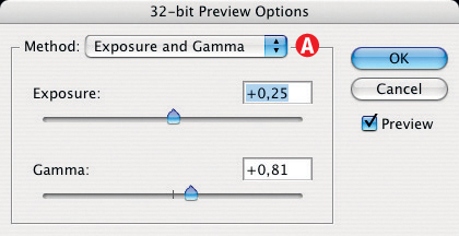
Figure 6-28: Choosing the tone mapping display method for 32-bit images.
![]() Tone Reproduction Curves are explained in detail in Christian Bloch’s HDR book [4] oral www.fdrtools.com/documentation/creating_profiles_d.php
Tone Reproduction Curves are explained in detail in Christian Bloch’s HDR book [4] oral www.fdrtools.com/documentation/creating_profiles_d.php
The dialog shown in figure 6-26 (setting ![]() ) can also be used to determine whether Photoshop calculates a tonal response curve based on the loaded images, or whether it uses a preset response curve.* Tonal response curves (also called Tonal Reproduction Curves, or TRCs) describe the way the camera’s sensor reacts to differing brightness values within the visible spectrum, and allow the source images to be linearized. If your source images are already stored in a linear form (as are RAW image files), response curve analysis is no longer necessary.
) can also be used to determine whether Photoshop calculates a tonal response curve based on the loaded images, or whether it uses a preset response curve.* Tonal response curves (also called Tonal Reproduction Curves, or TRCs) describe the way the camera’s sensor reacts to differing brightness values within the visible spectrum, and allow the source images to be linearized. If your source images are already stored in a linear form (as are RAW image files), response curve analysis is no longer necessary.
We recommend using the automatic setting, as shown in figure 6-26. If your images contain relatively neutral colors, automatic mode will function adequately. However, if an image is dominated by a single, strong color (when shooting a sunset, for example), automatic mode can deliver unsatisfactory results. To avoid this, we recommend saving and using the automatically generated response curve from a bracketing sequence with a broad dynamic range. You can then load this curve into your more problematic images later. You can also achieve a similar result if you shoot a separate image sequence of a neutral gray card, shot using different exposure values, and with the lens deliberately left out of focus. You can then merge this sequence into an HDR image using Photoshop, and save the curve generated automatically by the process for later use.
Unfortunately, stored response curves cannot (yet) be transferred between different HDR programs.
Returning to our HDR creation dialog box in figure 6-26: if you have chosen the 32 Bit/Channel option, you will be able to use a number of further enhancements in Photoshop CS3 or CS4 (although, as mentioned, most 32-bit filters and tools are only available in the “Extended” versions of the program). Keep in mind that the image being displayed is the result of a provisional tone mapping process, making it difficult to make accurate visual judgments. You will here have to rely much more on the quoted tonal values and histogram displays for reliable image information.
![]() Unfortunately, Photoshop CS2, CS3, and CS4 do not display histograms for 32-bit images via Window ▸ Histogram. In order to view a 32-bit histogram, you need to create a Levels adjustment layer.
Unfortunately, Photoshop CS2, CS3, and CS4 do not display histograms for 32-bit images via Window ▸ Histogram. In order to view a 32-bit histogram, you need to create a Levels adjustment layer.
One advantage of a 32-bit export format is that you won’t have to rely solely on the Photoshop tone mapping tools. There are a number of other specialized Photoshop plug-ins which are compatible with 32-bit HDR images, such as Enhancer by Akvis [18], Tone-Mapper by HDRsoft [13] or FDRCompresser by Andreas Schömann [24]. (At the time of press, a Photoshop CS3- or CS4-compatible version of FDRCompressor was not yet available.)
But for now, we will stick to Photoshop, as we will, at some point, have to reduce our 32-bit image to a 16- or 8-bit format for printing, reproduction at a photo lab, or display on the web.
Once the images have been merged, the program displays a preview HDR image similar to the one we have already seen. The limitations of computer monitor technology make it impossible to display the entire dynamic range of the actual HDR image. Our reproducible image will only become visible once we have tone-mapped it to an 8- or 16-bit format. We now need to save our original HDR image so that we can safely try out various different tone mappings. The saved HDRI file can then be converted and tone mapped using other tools*, such as Photomatix Pro or FDRTools.
HDRI File Formats
When saving our HDR image using File ▸ Save As, we have a number of different formats at our disposal (see figure 6-29), ranging from standard Photoshop PSD to a specialized 32-bit TIFF format. Each of these formats has specific advantages and disadvantages. A detailed explanation would be beyond the scope of this book, but Christian Bloch’s HDRI book [4] provides further, comprehensive information on the subject.
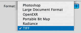
Figure 6-29: Photoshop (here CS3) offers a number of different HDR output formats.
Our choice is guided by two separate considerations: the size of the resulting image files and compatibility with the other programs we wish to use. Table 6-2 contains information related to these issues. There are also a number of HDRI formats that are not supported by Photoshop – for example, the very compact JPEG-based format. Table 6-2 does not include information on formats that are not supported by Photoshop.
Table 6-2: File Size and Compatibility of Various HDRI File Formats1 |
|||||
Format/Program |
Compression |
Photoshop |
Photomatix |
FDRTools |
HDRI Viewer |
Photoshop (.psd) |
None |
|
– |
– |
Only Bridge |
PSD-Large (.psb) |
None |
|
– |
– |
Only Bridge |
OpenEXR (.exr) |
High (various) |
|
|
|
Many |
Portable Bitmap (.pbm) |
None |
|
– |
– |
Few |
Radiance (.hdr) |
Good |
|
|
|
Many |
Portable Floating Map (.pfm) |
None |
|
– |
– |
Few |
32-Bit-TIFF (.tif) |
Various compression types |
|
Several (depending on the format variant) |
||
1 This information is based on Photoshop CS3/CS4 Extended, Photomatix Pro Version 3.03, and FDRTools Advanced Version 2.2.
2 Not all variants of the TIFF formats supported by Photoshop are also supported by the other programs mentioned. We recommend using the “32 Bit (Float)” method with LZW Compression.
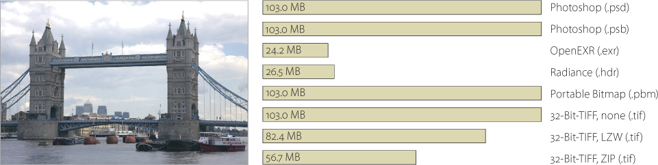
Figure 6-30: The selected format determines how large our HDRI file will be. The compression factor may, however, vary from image to image.
There are also a number of compression and compatibility options available when saving HDR images as TIFF files in Photoshop.
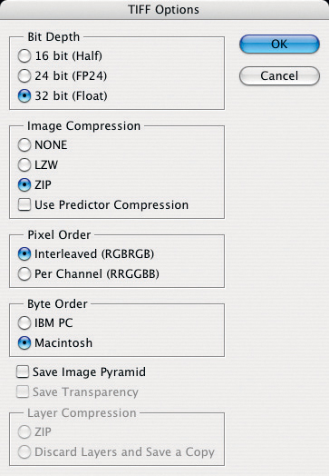
Figure 6-31: Photoshop offers a number of options when saving 32-bit HDR images to TIFF.
If you save your images in OpenEXR, Radiance, or Floating Point TIFF (also known as 32 Bit TIFF) formats, the resulting files will be compatible with other HDR programs, whereas HDR-PSD, HDR-PSB, and HDR-PMB are supported almost exclusively by Photoshop. Radiance and OpenEXR are probably the most useful formats when it comes to striking a good compromise between compression and compatibility.
Should you choose to save your HDR image as an HDR TIFF file, you will be presented with a long, possibly confusing list of options (see figure 6-31). We use the 32-bit (Float) option with LZW compression, as experience has shown that this combination yields relatively compact files with good compatibility characteristics.
In order to differentiate more easily between HDR TIFF and normal TIFF files, we attach the additional “HDR” suffix to our file name – for example: TowerBridge_HDR.tif.
As well as the programs that generate HDR images, there are also a number of dedicated HDRI viewers available, covering a wide range of different HDR formats. The Adobe Bridge image browser, for example supports the same formats as Photoshop. Other free viewers include Preview (![]() , the Mac OS X image viewer), HDR View (
, the Mac OS X image viewer), HDR View (![]() , [26]), OpenEXR Viewer (
, [26]), OpenEXR Viewer (![]() , [25]), XnView (
, [25]), XnView (![]() ,
, ![]() , [27]), and IrfanView (
, [27]), and IrfanView (![]() , [28]). Not all of these viewers, however, provide the same levels of speed and viewing quality.
, [28]). Not all of these viewers, however, provide the same levels of speed and viewing quality.
Processing and Optimizing HDR Images
HDR images can be optimized using Photoshop, but not all of the typical Photoshop functions are available for this type of image. In Photoshop CS3, many adjustment layers and filters are not 32-bit compatible. The full repertoire of 32-bit functionality is only available in the “Extended” versions of Photoshop CS3 and CS4.*
Image cropping and rotation is still possible, as is use of the Stamp tool (for removing sensor dust flecks, for example). Although the (CS3/CS4 Extended) Lens Correction filter isn’t available, several of the transformation functions used for correcting perspective distortion are. In our example, we started by straightening the image (using the ![]() tool, and then Image ▸ Image Rotation ▸ Arbitrary). We then corrected the perspective distortion in the bridge’s towers using the free transform tool (Edit ▸ Free Transform). The Hue/Saturation command is also available, and can help you correct specific image areas selectively. For example, by reducing the luminance of an otherwise flat-looking blue sky.
tool, and then Image ▸ Image Rotation ▸ Arbitrary). We then corrected the perspective distortion in the bridge’s towers using the free transform tool (Edit ▸ Free Transform). The Hue/Saturation command is also available, and can help you correct specific image areas selectively. For example, by reducing the luminance of an otherwise flat-looking blue sky.
The middle section of figure 6-32 shows the range of adjustment layers that support 32-bit files. One of the most important functions is Exposure (see Photoshop Help for more information). However, if you make use of adjustment layers and want to retain the layer structure of your HDR image, you will have to save to PSD, PSB, or 32-bit TIFF, which will, in turn, destroy any compatibility with other HDRI programs. We therefore recommend that you merge your image into a single layer before exporting it for processing in other (non-Adobe) programs.
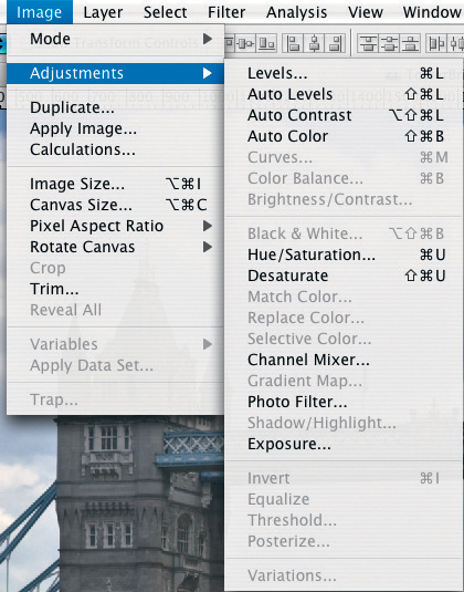
Figure 6-32: Not all Photoshop corrections are available when working with 32-bit images.
Sharpening is also an option, either using the USM filter (Filter ▸ Sharpen ▸ Unsharp Mask) or Filter ▸ Sharpen ▸ Smart Sharpen. As a rule, though, we only sharpen our images as a very last step – usually after the image has been scaled for output. We therefore very rarely sharpen HDR images. Uniform, minimal sharpening can be applied to all images in a sequence at an earlier stage using a RAW converter.
However, the problem of visual inspection of the largely inadequate preview image remains. This is especially relevant in the case of corrections to color and hue. As previously mentioned, the 32-Bit exposure slider in the bottom left corner of the preview window can help you gain a better overall impression of your image.
It is nevertheless worth the effort to correct your images in 32-bit mode, as you will then have the largest possible reserves of quality and color depth. As a result, many of the potential negative side effects of your corrections will not be visible in the final image. Image alignment, for example, is best performed directly on HDR images (provided it hasn’t already been applied using Lightroom or Adobe Camera Raw). Adjustments made using ACR or Lightroom can be transferred to the other images in a sequence using the Synchronize command.*
The same is true for cropping. Cropping can reduce the amount of data in a file, which can, in turn speed up processing in general.
As already mentioned, the 32-bit exposure slider in the preview window (see figure 6-33) can greatly improve the rendering of your preview image, helping you to get a better overall impression of your HDR image. This tool is very important to the decision-making process when correcting HDR images. But remember, the slider setting only affects the preview image, not the image file itself.
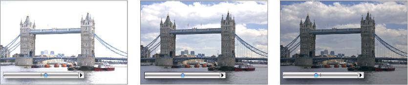
Figure 6-33: The “32-bit Exposure” slider in the Photoshop preview window provides a simple way to adjust the lighting in a preview image without actually changing the image file. This helps when planning decisions about exposure corrections.
Tone Mapping HDR Images
The next important step is tone mapping. This process (illustrated in figure 6-34) reduces the increased dynamic range of your HDR image to that of a 16- or 8-bit LDR (Low Dynamic Range) image. The resulting LDR image can be reproduced more naturally and is supported by a much larger range of processing functions and filters. Printing is also currently only possible for 8-bit images, or (with some limitations) 16-bit images.
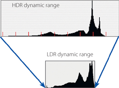
Figure 6-34: Converting from HDR to LDR reduces the dynamic range of an image to 8 or 16 bits per color channel. The details of the algorithms used to do this remain the secret of the software companies who make them.
The dialog shown in figure 6-35 will appear when using Photoshop to convert an image from 32-bits to 16- or 8-bits. It can be accessed from the dialog box shown in figure 6-35 or through Image ▸ Mode ▸ 16 Bits/Channel. Here, you can select your tone mapping method, and the results of your selection are displayed directly in the preview window. There are four tone mapping methods available in Photoshop CS3 and CS4. These are called Exposure and Gamma, Highlight Compression, Equalize Histogram, and Local Adaptation.
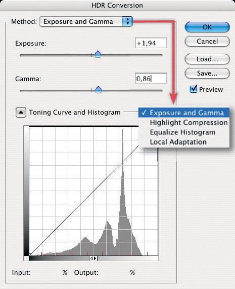
Figure 6-35: Photoshop CS3 provides four methods for tone mapping 32-bit images for 16- or 8-bit output. The expandable histogram view shows the range and distribution of tonal values within the selected image.
The best way to choose a method is to experiment and see which suits your personal taste and your type of images best. Not every method works equally well for every type of image.
We have already seen the Exposure and Gamma and Highlight Compression options in the 32-bit HDR tone mapping preview window. Figure 6-35 shows the Exposure and Gamma tone mapping dialog. The default settings will correspond to the settings you made in the white point preview. Our initial goal will be to find an Exposure value which clips highlights as little as possible. The degree of clipping you are prepared to accept will depend largely on the subject you are portraying.
The sliders react quite sensitively to movement, so we prefer to click on the numerical value box and use the arrow keys (![]() ,
, ![]() ) to make changes. This allows for much greater precision. Holding down the
) to make changes. This allows for much greater precision. Holding down the ![]() key while changing the value will increase the size of the increment.
key while changing the value will increase the size of the increment.
A flat-looking image is more easily corrected than an image with too much contrast – even if the high-contrast image is more immediately visually appealing. Figure 6-36 shows the results of using the described settings, which have reduced the tonal range in some of the cloud formations.
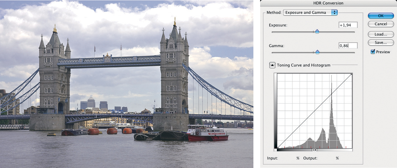
Figure 6-36: The result of “Exposure and Gamma” tone mapping using the values shown above.
In any process involving sliders, remember to make changes slowly to allow Photoshop time to update the preview.
The Highlight Compression and Equalize Histogram methods do not have any dedicated sliders and therefore appear to be simple and less configurable. This isn’t necessarily true, and Highlight Compression works well if you simply want to enhance highlight detail. However, images with broader dynamic range can turn out quite dark, as shown in figure 6-38.
The Equalize Histogram method shares some aspects of its methodology with the Photoshop Auto Tone command, which attempts to optimize contrast by stretching the portions of the histogram that contain more pixels. This can only be achieved at the expense of the portions of the histogram which contain less pixels, which are then correspondingly compressed. The result is an equalization of the tonal values and a compression to 16- or 8-bit dynamic range.
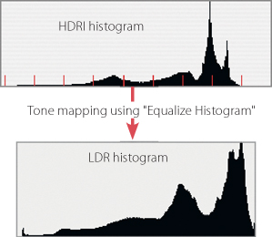
Figure 6-37: Histogram of the LDR-imge after applying “Equailze Histogram”.
Images which have only moderate dynamic range can usually be effectively optimized using Photoshop. Figure 6-39 shows the results we attained using this process. It is obvious that here, the extreme shadow and highlight tones have been too highly compressed, creating a flat, somewhat lifeless image.
The three tone mapping processes we have described apply a global tone mapping which processes all pixels with the same tonal value uniformly, resulting in a new LDR image in which all these pixels also have the same (possibly changed) value.
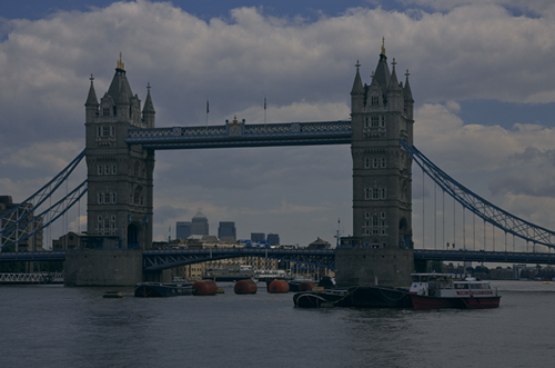
Figure 6-38: The result of our tone mapping using the “Highlight Compression” method.
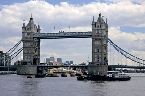
Figure 6-39: The result of our tone mapping using the “Equalize Histogram” method.
You can usually achieve better results if the algorithm you use takes neighboring pixels into account. This type of method is described as localized tone mapping.
Photoshop offers the Local Adaptation tone mapping method for exactly this purpose (see figure 6-40). This is the most versatile method. In addition to the Radius and Threshold sliders, you can also use a gradation curve to fine-tune your adjustments. (The gradation curve that can be displayed in the other tone mapping dialogs can be viewed but not edited.) We use this method to tone map most of our images. We begin by moving the black point to the far left, and the white point to the far right of the available tonal range using option ![]() Toning Curve and Histogram (see figure 6-40).
Toning Curve and Histogram (see figure 6-40).
If you click on the brightest and darkest points of your image using your mouse, Photoshop will indicate the position of the equivalent luminance value on the gradation curve with a small circle icon. However, the histogram can be misleading, especially in the highlight areas, which are sometimes hard to identify, and thus easy to clip. Using the eyedropper tool together with the info window (Window ▸ Info) and the circle marking in the Local Adaptation window (see figure 6-42) can often provide more accurate analysis of your image than a purely visual approach. Once the black and white points have been set, we can start experimenting with the Radius and Threshold sliders.
During this process, Photoshop generates a brightness map, which is never actually seen by the user, and which works similarly to a soft-focus filter. The Radius controls the size of the area around each pixel which is taken into account while tone mapping – setting the value to “1” will only include the four immediately neighboring pixels.
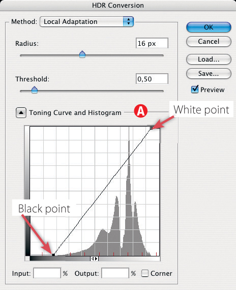
Figure 6-40: We begin the “Local Adaptation” process by setting the black and white points.
Figure 6-41: The “Local Adaptation” tone mapping method uses a virtual luminance mask.
The Threshold value controls the degree of blur, or, more accurately, how great the difference in tonal values between neighboring pixels should be in order that they become grouped and equalized. In other words, the threshold value sets the maximum difference in brightness between neighboring zones within the image. The threshold value here has nothing to do with the sharpness of the image.
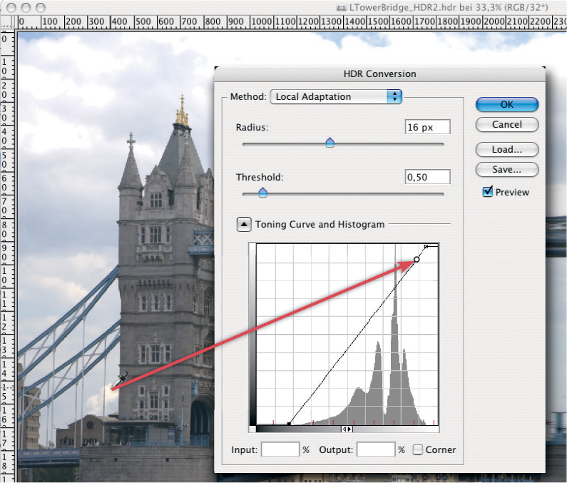
Figure 6-42: Using the eyedropper tool to click in the image sets a marker at the corresponding luminance value in the HDR conversion histogram. This only works with the “Local Adaptation” method.
Figure 6-43: A halo effect can appear at high-contrast edges if the threshold and radius values are set too high.
A higher threshold value – strengthened by a large radius – can soon lead to halo effects appearing at high-contrast edges, as illustrated in figure 6-43.
Unlike the standard gradation curve, the Local Adaptation tone mapping method does not process all pixels of a certain luminance uniformly. Instead, it couples the effect of the gradation curve with that of the luminance mask, making a certain amount of experimentation necessary to find the right levels for your particular image. As with all other complex processes, it pays to vary the slider values slowly, so Photoshop has time to update the preview between changes.
Finally, we fine-tune the gradation curve, as illustrated in figure 6-44. This is a process that requires a good deal of trial and error while you search for the place on the curve where the tonal value of a specific image area lies.
Normally, Photoshop smooths the curve. You can, however, create corners in the curve by creating a new point and activating the Corner option (see ![]() in figure 6-44). This is not an effect you would want to apply to most normal gradation curves. As in the standard Photoshop Curves dialog, a curve point can be removed by selecting it and pressing delete.
in figure 6-44). This is not an effect you would want to apply to most normal gradation curves. As in the standard Photoshop Curves dialog, a curve point can be removed by selecting it and pressing delete.
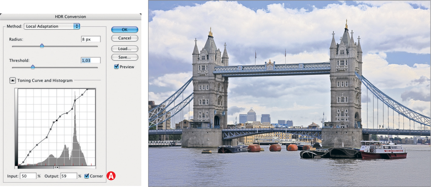
Figure 6-44: Our image after “Local Adaptation” tone mapping using the settings shown on the left. Unfortunately the sky is still a little bland, so we will optimize it later using Photoshop.
Figure 6-44 shows only one of many possible versions of our original HDR image. We used Photoshop to improve color rendering (using the Hue/Saturation command) and heightened contrast slightly before enhancing the details on the bridge structures using DOP Detail Extractor*. We protected the sky from unwanted filter effects using a layer mask during this process, and the result can be seen in figure 6-45.
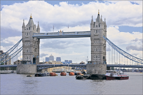
Figure 6-45: Our sharpened image after post-processing with Photoshop.
Instead of converting an HDR image to LDR using Photoshop’s tone mapping function, you may want to use a third party filter. HDRsoft’s [13] Tone Mapping filter is a good choice. This plug-in delivered better results than Photoshop for the example shown here. The Tone Mapping plug-in’s handling is very similar to that of the Details Enhancer in Photomatix Pro, so we decided not to describe it in detail here.
That concludes our discussion of Photoshop-based HDR techniques. Because of its superior loading and aligning functionality, we often use Photoshop to generate HDR images that we later process using either Photomatix Pro or FDRTools.
Optimizing HDRI Processes
Even today’s faster computer systems require a considerable amount of time when processing HDR images, although Photoshop is definitely one of the faster programs available. For most of the processes described here, it is necessary to experiment with different combinations of settings. One way to save time is by trying out your ideas on scaled-down images before applying them to your full-sized image files.
It is possible to save and reload Photoshop settings for HDR and most other corrective processes. This can save a lot of time if you are processing multiple images. Photomatix Pro and FDRTools have a similar function, which can be used in a special batch-processing mode.
![]() Bear in mind that the effects the “Local Adaptation” settings have (especially the “Radius” setting), depend very much on the resolution of the original image.
Bear in mind that the effects the “Local Adaptation” settings have (especially the “Radius” setting), depend very much on the resolution of the original image.
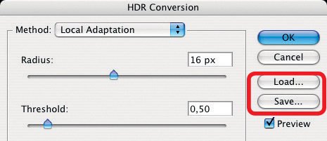
Figure 6-46: Photoshop (and other HDRI tools) allow you to save settings for later use.
6.6 HDR Imaging Using Photomatix Pro
HDRsoft’s Photomatix Pro [13] is one of the best currently available HDRI tools. The program is available for Windows and Mac OS X (both Intel-based and PowerPC-based systems). It is powerful and fast (although not quite as fast as Photoshop) when processing complex HDRI algorithms. As with all HDRI tools, a fast processor and plenty of RAM are an advantage when working with Photomatix Pro.
HDRsoft also offers “Photomatix Basic” (for Windows) as a free download. The program can create and tone map HDR images but is less versatile than its Pro counterpart. We will therefore stick to describing Photomatix Pro in this book.
Photomatix Pro is a stand-alone program, and is complemented by its sister product, the Tone Mapping Photoshop plug-in. This can be used to tone map 16- and 32-bit HDR images using Photoshop CS2 or CS3.* Compatible source programs include PhotoAcute, FDRTools, and Photoshop. Even if the Pro version of the program is too expensive for you, you should at least give the Photoshop plug-in and the Basic version a try.
![]() There is also a free Lightroom plug-in for Photomatix Pro, that allows you to directly export images form Lightroom 2 to Photomatix Pro.
There is also a free Lightroom plug-in for Photomatix Pro, that allows you to directly export images form Lightroom 2 to Photomatix Pro.
The stand-alone version of Photomatix Pro 3.1 supports a range of LDR input formats including JPEG, 8-, and 16-bit TIFF files, and a number of RAW formats (including DNG). If you want to adjust white balance, remove aberrations, crop, or otherwise preprocess your RAW files, please bear in mind that Photomatix cannot interpret corrections made using Adobe Camera Raw or Adobe Lightroom, as these changes are either embedded in the DNG file itself or reside in an XMP sidecar file. As is the case with PhotoAcute (and other RAW processing software), the program can only interpret the original RAW image data. We therefore recommend that you export your images to 16-bit TIFF before processing them with Photomatix Pro.
Personally, we are not particularly fond of the results that Photomatix Pro’s dcraw RAW converter delivers. We almost always use 16-bit TIFF source files, but, as always, this type of decision is matter of taste and requires experimentation.
It is only occasionally advantageous to work with 8-bit JPEG files. If this is your input format, PhotoAcute is probably your best choice of software tool.
Photomatix Pro is augmented by a very good online help function, as well as an online tutorial and a comprehensive online user manual, which is useful both as an introduction and a working guide to the program.
As usual, you should navigate to the program’s Preferences dialog when using it for the first time (see figure 6-47), where the available tabs and settings are generally self-explanatory. On the RAWs tab, we recommend setting Demosaicing Quality to High (if you prefer to use RAW source files rather than TIFFs). Here, you can also set your preferred output color space (we use either Adobe RGB or ProPhoto RGB).
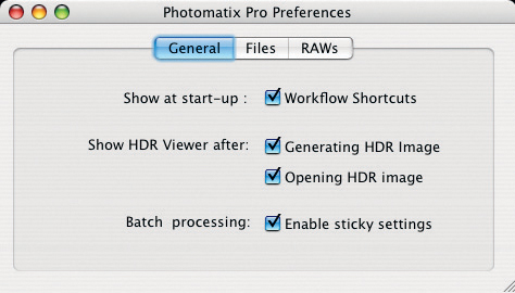
Figure 6-47: You can select your own personal preferences when using Photomatix Pro for the first time.
When starting Photomatix Pro, the first thing you will see is a toolbar containing workflow shortcuts (figure 6-48). Here, Photomatix Pro offers four basic options:
▸ Generate an HDR image from multiple source files
▸ Tone mapping for existing HDR images
▸ The Exposure Blending function (see page 170)
▸ The batch conversion of LDR images to HDR images and (optional) tone mapping of HDR images to LDR images
There is a Tutorial button included in the tool bar. Instead of using the toolbar dialog, you can also open images in Photomatix Pro by simply dragging them to the program’s icon, or by using the new Lightroom export plug-in to load images directly from Lightroom 2. If this option is selected in the program’s preferences, Photomatix Pro opens a new dialog window, and asks which process should be applied to the freshly loaded images.
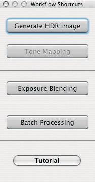
Figure 6-48: The Photomatix workflow shortcut panel offers four basic functions.
Generating HDR Images Using Photomatix Pro
For our example we will use three images of the Swiss Re building taken across the Thames River in London. Figure 6-49 shows the source images and their corresponding histograms.
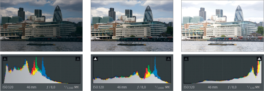
Figure 6-49: The three (16-bit TIFF) source files for our HDR image. The building that looks like a Faberge egg is, in fact, the famous Swiss Re “Gherkin” building.
If we now click the Generate HDR Image button, the program will open a dialog box in which we can select our source images. As ever, this is easier if the relevant source images are grouped in a single folder.
In the next dialog box (see figure 6-50 and 6-51), we select our image processing options, including alignment type, ghosting removal options, and the type of gradation curve we wish to apply.

Figure 6-50: Setting the HDRI generation options in Photomatix Pro.
We use the Align source images By matching features option for most of our images.
The settings for avoiding ghosting artifacts should be largely self-explanatory. Grass and leaves blowing in the wind and fast-moving clouds should be thought of as background movement. If your shot includes moving cars or people, you can use menu ![]() (see figure 6-50) to set a higher level of detection. Higher levels will lead to longer processing times and don’t always improve the results.
(see figure 6-50) to set a higher level of detection. Higher levels will lead to longer processing times and don’t always improve the results.
With regard to the tone response curve (TRC) – already mentioned on page 152, and here called the tone curve – we recommend using the default setting, which generates a curve based on the color profile stored in your image.
If you are using RAW source files, you will be able to set the additional options shown in figure 6-51. These relate mostly to white balance and color space. As most cameras select and embed the correct white balance (color temperature) setting directly into the RAW image files – at least when shooting outdoors in daylight, as was the case in our example – you should set white balance As Shot.
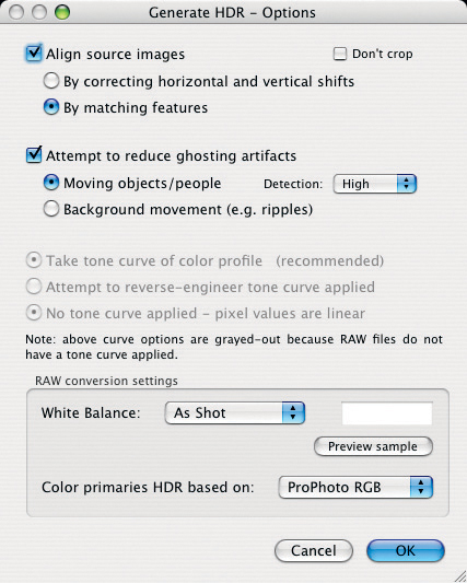
Figure 6-51: The additional options available for processing RAW files.
Otherwise, you can select an appropriate color temperature from the list in the White Balance dropdown list. It is also possible to set white balance later during tone mapping – an option that gives us better visual control. We usually select the ProPhoto RGB option for Color primaries because it offers the largest color space. We will transform our image into a smaller color space later (after the tone mapping), once we have scaled our image for output. ProPhoto RGB is not a suitable color space for use with 8-bit images. 8-bit images (JPEGs, for example) are better processed using the Adobe RGB or sRGB color spaces.
Clicking the OK button in the dialog box shown in figure 6-50 (or 6-51) will then generate an HDR image and display it in a preview window (see figure 6-53). As with most HDR programs, the preview image is only provisionally tone mapped. The HDR Viewer window provides a better quality display, although it only displays a small detail of the entire image. The image displayed is based on the last mapping process that was applied by the program.
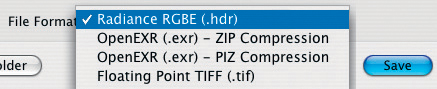
Figure 6-52: Photomatix Pro 3.0’s HDR output formats.
We now save our new HDR image using File ▸ Save HDR As. In addition to the Radiance and OpenEXR formats, Photomatix Pro offers the 32-bit floating point TIFF output format (see figure 6-52). This is equivalent to the Photoshop “32 Bit (Float)” format, but we generally use the Radiance format in order to preserve the greatest possible compatibility.
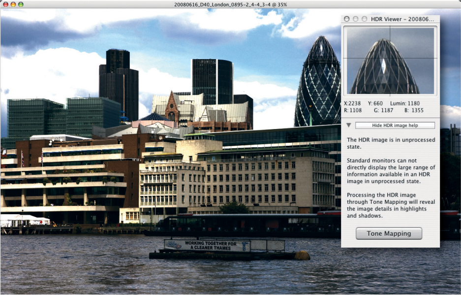
Figure 6-53: The first preview version of our HDR image. A better view can be seen in the detail displayed in the HDR Viewer window.
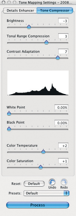
Figure 6-54: The control panel for “Tone Compressor” tone mapping.
We use Photomatix Pro for the actual tone mapping, because of its known strengths in this area. Click Tone Mapping – either in the workflow shortcut panel or the HDR Viewer window – to generate a preview version of the image. Another loupe window will now appear (see figure 6-57 on page 167). We then set the size of the preview image using the buttons at ![]() , and we can switch between the tone mapping preview and the original HDR image using the button
, and we can switch between the tone mapping preview and the original HDR image using the button ![]() .
.
If you’re running Photomatix Pro on a slower computer, you can gain some speed by setting option ![]() to Refresh loupe only. This way, you won’t have to wait for the entire preview window to be updated after every change.
to Refresh loupe only. This way, you won’t have to wait for the entire preview window to be updated after every change.
Again, the preview only shows a provisional tone mapping, but this time the details are determined by the settings made in the mapping panel. Photomatix Pro offers two different tone mapping processes: Details Enhancer and Tone Compressor. Both have many more control options than Photoshop, making the Photomatix tone mapping process more versatile, but also more complex.
Tone Mapping Using “Tone Compressor”
The Tone Compressor global tone mapping method is similar to Photoshop’s Highlight Compression process, but offers more settings, as can be seen in figure 6-54. Here, we start by setting the black and white points. Although we can also use the current panel to adjust Color Temperature and Color Saturation, the actual compression and tonal value adjustment are controlled using the Tonal Range Compression and Contrast Adaptation sliders.
These settings alone will produce a better result more quickly than we could have achieved using Photoshop (even using Local Adaptation). Figure 6-67 shows our initial result, which could nevertheless do with some further optimization.
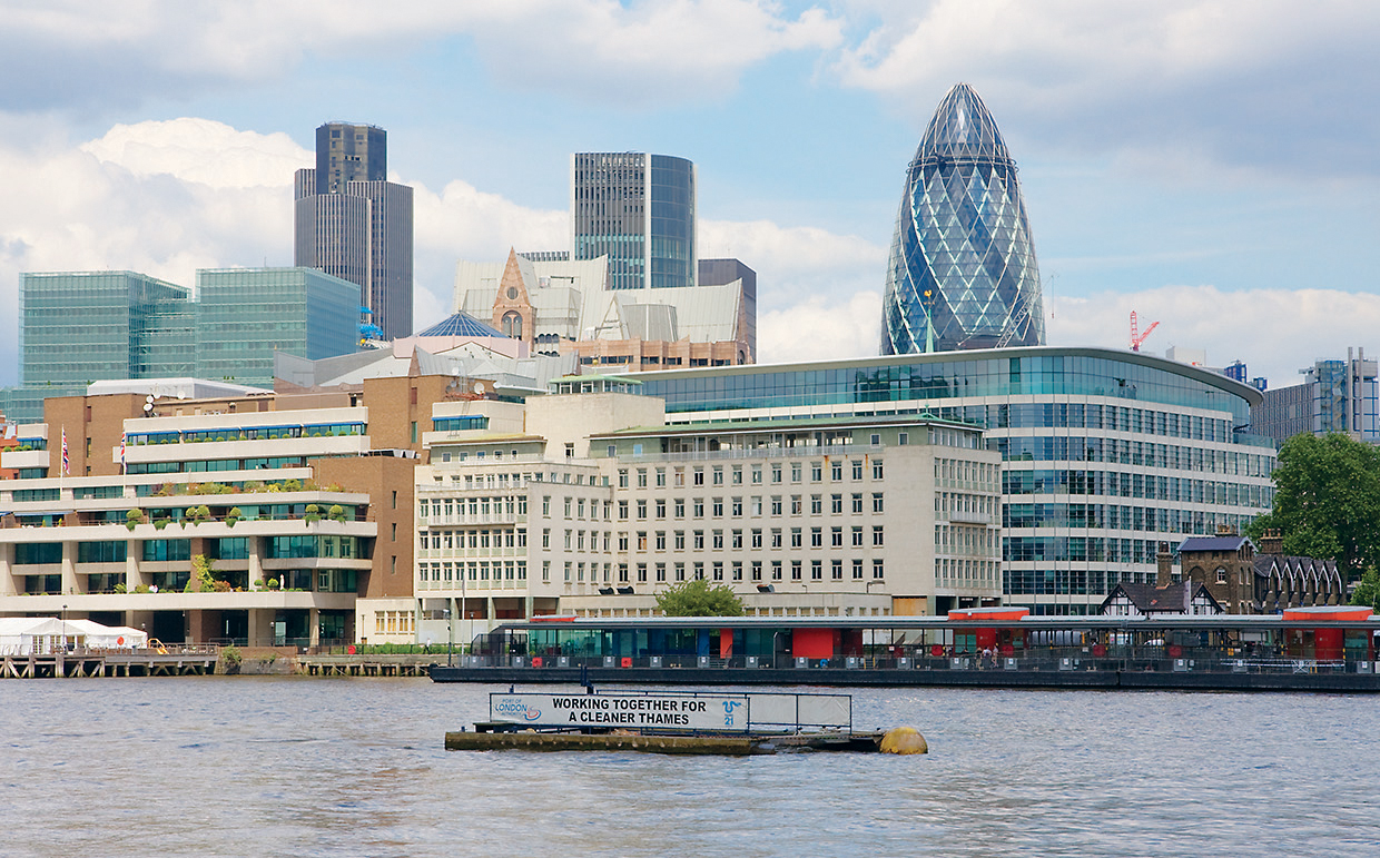
Figure 6-55: Our image after tone mapping in Photomatix Pro using “Tone Compressor”.
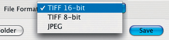
Figure 6-56: Photomatix Pro’s LDR output formats.
But we are still viewing a preview. The actual resulting image can be different in a number of details. It is therefore necessary to convert our image to LDR in order to be able to view the actual results using either Photomatix Pro itself or Photoshop. Start the conversion from HDR to LDR by clicking the Process button in the tone mapping panel (see figure 6-54).
You can then save your image using File ▸ Save as (see figure 6-56). We always use TIFF 16-bit as our LDR export format.
Tone Mapping Using “Details Enhancer”
The real strength of Photomatix Pro lies in the Details Enhancer tone mapping option. Using this tone mapping method often gives us a typical HDRI “grunge” look for many images, an example of which can be seen in the preview window shown in figure 6-57.* The illustration next to it shows the Details Enhancer tone mapping control panel.
The Details Enhancer method applies a localized tone mapping similar to Photoshop’s Local adaptation, also recognizable from the similarities between the controls offered by both processes.
We start by setting Strength to a moderate, mid-range value. The default value (70) is often a good starting point, but your results will be more natural-looking if you use values of 50 or less. We then need to make our basic settings for the black and white points, which we can fine-tune later if necessary – the higher the values we set, the more highlight and shadow detail will be clipped.
A good working gamma value is 1.0. Higher values will lead to higher-contrast images, while lower values will produce duller results – which is not always a bad thing. Here too, you will need to be patient while waiting for your preview image to refresh. It is all too easy to over-correct your image if you try to work too fast.
![]() It’s much easier to increase contrast later using Photoshop. Artificially decreasing contrast is virtually impossible.
It’s much easier to increase contrast later using Photoshop. Artificially decreasing contrast is virtually impossible.
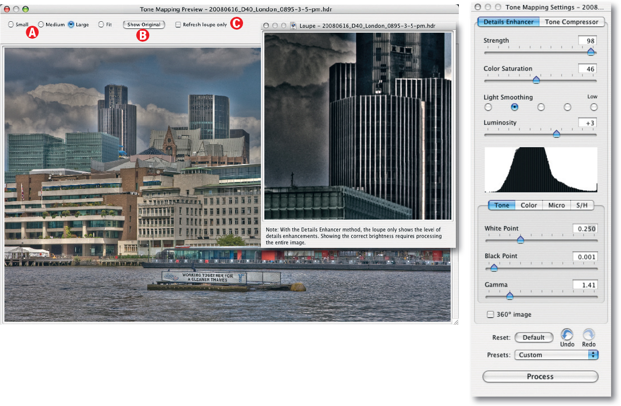
Figure 6-57: The preview of our first “Details Enhancer” tone mapping with the activated HDR Preview window. The look of the preview image results from a high “Strength” value.
Before we start adjusting the color saturation, we navigate to the Color tab to make any necessary adjustments to color temperature (see figure 6-58). We then adjust the color saturation for highlights and shadows. Minor increases can make your image much more vibrant, but overdoing things will quickly give your image an artificial and obtrusive look.
We then switch to the Micro tab (see figure 6-59) to adjust the microcontrast (or local contrast) level. For more information regarding micro-contrast, see chapter 7. Increasing microcontrast at this stage can make your image appear more lively, and will cut out one of the post-processing steps you would otherwise have to go through later.
One disadvantage of setting microcontrast within Photomatix is that the changes you make are then applied to the entire image, whereas you can use Photoshop masks to enhance microcontrast selectively at the post-processing stage. If you are using high Strength values, you may also need to increase the level of Micro-smoothing to keep the microcon-trast effect under control.

Figure 6-58: Detail of the Photomatix Pro tone mapping control panel, with the “Color” tab activated.
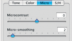
Figure 6-59: The “Micro” tab in the Photomatix Pro tone mapping control panel.
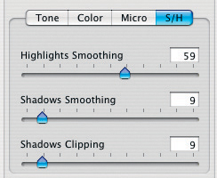
Figure 6-60: Settings for shadows and highlights.
The last fine-tuning tab is the S/H (Shadows and Highlights) tab (see figure 6-60). You can set Shadows Clipping higher if you are prepared to trade some shadow detail for increased contrast and more shadow saturation. The best settings for your image will depend on the subject itself and your personal taste. Increasing the Highlights Smoothing and Shadows Smoothing values can help to avoid shadow and highlight clipping by adjusting the range of highlights or shadows that contrast enhancements are applied to. Moving the loupe over the corresponding sections of the image can help to determine the best values to use, as shown in figure 6-61.
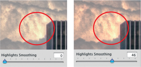
Figure 6-61: In the left-hand image, the tonal values in the clouds are clipped. This was remedied in the image on the right using the “Highlights Smoothing” slider.
We can now go back to the main settings and once again adjust the Strength setting. The best value to use here is also largely a matter of taste. Many published HDR images are vilified for their exaggerated and sometimes unnatural look – which applies to some of the images in this book too. However, if you set a moderate Strength value (of 50 or less), you should be able to avoid the more pronounced effects that HDR processes can produce.
Another disadvantage of higher Strength values is the increased image noise they produce. We therefore recommend that you keep your Strength values low and that you instead shoot at low ISO speeds whenever possible.
We now move on to the Color Saturation, Light Smoothing, and Luminosity settings (see figure 6-62). As a final step, we may readjust the Gamma value.*
Setting the Light Smoothing control to a higher value can lead to more natural-looking results for high-contrast subjects and images with a generally higher dynamic range.
We have so far described the tone mapping steps you can take in a simple, sequential fashion. However, the reality of the situation is more complicated, as many of the settings described have knock-on effects on each other – which means that when you change one setting, the others react differently.
You should generally expect to have to make several attempts at a tone mapping before you find the optimum set-up. This will, however, help you to gain experience, and to develop your own style.
Once you have found a combination of settings that works well and might be suitable for other images as well, you can save it using the Presets dropdown menu ![]() (see figure 6-62). This will enable you to reuse the same values when processing similar images. This can save you a good deal of time, even if the resulting image still requires a little fine-tuning.
(see figure 6-62). This will enable you to reuse the same values when processing similar images. This can save you a good deal of time, even if the resulting image still requires a little fine-tuning.
As before, the actual tone mapping is activated by clicking Process in the tone mapping control panel. The results will then be displayed in the preview window.
The second tone-mapped interpretation of our HDR image is shown in figure 6-62. For this version, we used an extremely high Strength value of 98 when applying the Details Enhancer tone mapping method. The result is a slightly surreal-looking image. This image has already been slightly sharpened in Photoshop.
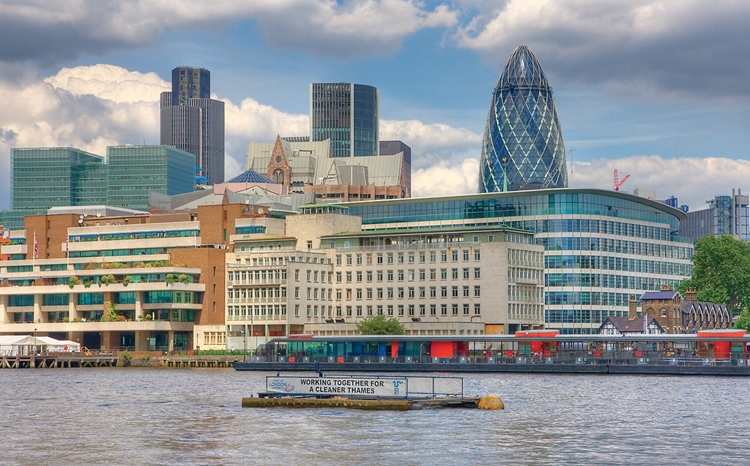
Figure 6-62: The second version of our image was created using the “Details Enhancer” tone mapping method and the settings shown on the left. The resulting image was then sharpened using Photoshop.
The emphasis here is definitely on the word “interpretation”, because the program’s numerous settings give you a very high level of flexibility in your work. The real indicator of a good result ought to be what the photographer saw or wanted to see while shooting. It is often necessary to shoot and process various versions of the same subject, depending on how the final image is to be used. The dramatic and almost oppressive sky in this image, for instance, is not suitable for every application.

Figure 6-63: Tone mapping settings used for the image in figure 6-62.
The Photomatix Pro “Exposure Blending” Function
A simple, but nonetheless useful HDR variant offered by Photomatix Pro is the Exposure Blending function. This function also merges source images with differing exposure settings, but outputs 8-bit or 16-bit LDR images. These images do not have to be reduced via tone mapping to a printable format. For this reason, this option is useful not only when shooting individual images for increased dynamic range, but also when shooting HDR series that you wish to stitch together in a panorama using normal stitching software.
This method also works well if you discover that no single image in a short bracketing sequence is exactly the image you envisioned. Instead of using the more complicated Photoshop blending/layer mask process described in section 6.3, simply use the Photomatix Pro’s Exposure Blending function.
You should use the same basic criteria you use for shooting other HDR source images when shooting images for use with this function. We usually use a small bracketing increment or, if we are only aiming to reduce image noise, no bracketing at all. If this is the case, we use the Average tone mapping method.
Figure 6-66 shows our two source images, shot in Death Valley. The first image has captured the sunrise nicely, while the second shows better detail in the salt flat.
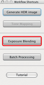
Figure 6-64: The Photomatix workflow shortcuts panel offers functions other than just HDR creation.
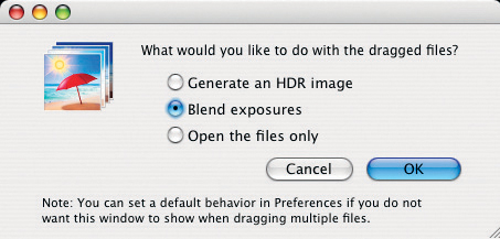
Figure 6-65: When you drag files onto the Photomatix icon the program will ask what process it should undertake.
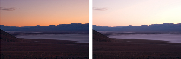
Figure 6-66: Our two source images of a Death Valley slat flat that we will use for “Exposure Blending”. The shots were taken two f-stops apart.
The process is started either by dragging your source images to the Photomatix Pro icon and selecting Blend Exposures (see figure 6-65), or by selecting the Exposure Blending workflow shortcut.
As with the HDR image creation process, the program will ask how the source images should be aligned. Even if you are working with a tripod, you should let the program align your images. In most cases (since Version 3), we use the By matching features option for image alignment.
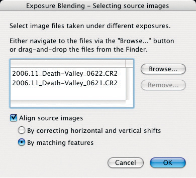
Figure 6-67: Selecting the exposure blending source files and the alignment options.
Photomatix Pro will load the files and temporarily blend them for preview in the dialog box shown in Figure 6-68. You can then select your blending method from the options offered in section ![]() of the window.
of the window.
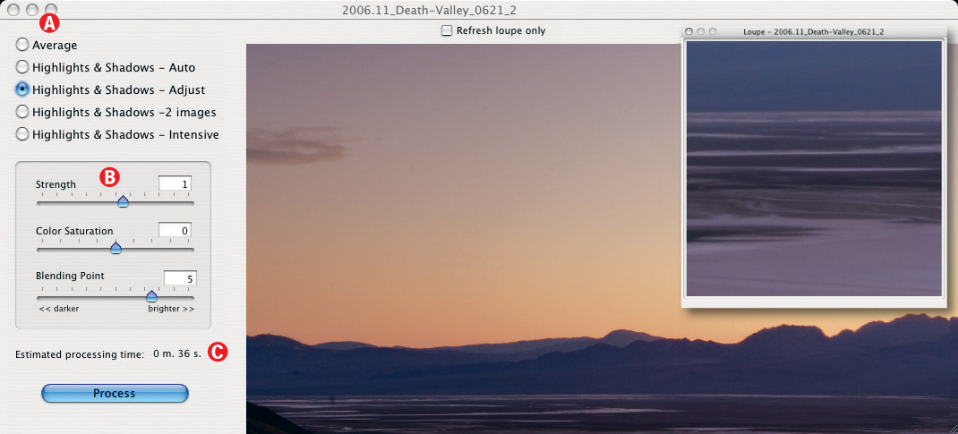
Figure 6-68: The Photomatix Pro “Exposure Blending” dialog offers five different blending methods, some of which have individual control parameters, as shown here.
The primary purpose of the Average method is to reduce noise. It is most useful for image sequences with largely similar exposure settings, or with small bracketing increments, or where the photographer had to use high ISO speed settings. Here, we are only interested in the resulting low-noise LDR image – a process we have seen before in PhotoAcute. It is equivalent to the PhotoAcute function: Combined 1x output (no super-resolution, noise reduction only). We don‘t generally use the Highlights & Shadows – Auto method, because it doesn’t allow any manual user control.
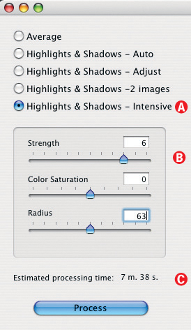
Figure 6-69: The parameter settings for the “Highlights & Shadows – Intensive” exposure blending method.
Our two favorite methods are Highlights & Shadows – Adjust and Highlights & Shadows – Intensive. We nevertheless recommend that you experiment with all the other methods too.
Processing time can vary substantially – from a couple of seconds to nearly an hour, even using the same source files. The actual time required depends on the number of images being processed, their size, the selected blending method and, of course, how powerful your computer is. Photomatix Pro estimates the remaining processing time and displays it in the program window (![]() ).
).
While the Photomatix Pro HDR function generates its HDR images from the various tonal value areas in the source images, the Exposure Blending function scans the source files to determine the source of every single pixel in the resulting image.
Our personal favorite method is Highlights & Shadows – Adjust, but we used Highlights & Shadows – Intensive for our example in figure 6-69. The Strength slider controls the microcontrast intensity. The Color Saturation control is self-explanatory. Radius defines the size of the area around each pixel from which the tonal values for the interpolation of the resulting image are taken. A larger radius will lead to longer processing times, but will reduce halo effects in high-contrast transitions and edges.
After experimenting, we selected the values shown in figure 6-69 and clicked the Process button. After nearly six minutes, the preview LDR image was displayed, which we then saved as a 16-bit TIFF file using File ▸ Save As. (The ![]() or
or ![]() keystroke is even faster.)
keystroke is even faster.)
Keep in mind that if you use 8-bit source images (JPEGs, for example), your results will also be 8-bit.
Figure 6-70 shows our resulting image, which we cropped a little at the top. This version is a definite improvement on our source images. The salt flat and the sunrise mountain peaks are both more clearly defined.
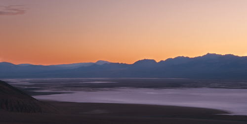
Figure 6-70: Our image after we applied the “Highlights & Shadows – Intensive” exposure blending method.
Batch Processing with Photomatix Pro
When you return from an extensive shoot with a lot of new HDR material, you may find the prospect of processing each of your sequences individually time-consuming and daunting. You will nevertheless want to get an overall impression of the sequences which warrant more work – which is where batch processing can be really useful. Using a batch process, you can run all of your image sequences through the processor using standard settings and then inspect the results for potential. You can then easily select your best images for manual processing
Photomatix has a useful, built-in batch processing function. The function does, however, rely on your source images being sorted according to specific criteria for it to work effectively. There are two ways of ensuring that this is the case:
![]() The Photomatix online handbook contains a good description of batch processing, which is why we’ve limited ourselves to a schematic description here.
The Photomatix online handbook contains a good description of batch processing, which is why we’ve limited ourselves to a schematic description here.
A. All your sequences contain exactly the same number of images. In this case you can save all of your images in a single folder and set the Photomatix Pro to batch process a particular number of images per sequence.
B. You save each sequence in its own subfolder, all of which are then placed in a main folder.
If you shoot sequences of very differing natures, it can be an advantage to create several folder structures in order to keep your HDR and Exposure Blending sequences separate.
You also need to decide whether your results should be saved in the same folder as the source images, or to their own, separate folder.
If you shot RAW images but want your source files to be in a preprocessed TIFF format, you will first need to process your images using a RAW converter. The exact process differs from converter to converter, so you will need to refer to your software manual for details.
Once you’ve organized your source material, you can start batch processing either by clicking the Batch Processing workflow shortcut button or by navigating to the Automate ▸ Batch Processing menu item. The dialog box shown in figure 6-71 will now be displayed. The available batch processing settings are as follows:
![]() Process type – HDR image generation or exposure blending. Here, you can select multiple processes, which then generate multiple results accordingly.
Process type – HDR image generation or exposure blending. Here, you can select multiple processes, which then generate multiple results accordingly.
The HDR option allows you to specify both tone mapping methods (Details Enhancer and another using Tone Compressor), which also produces multiple results if selected.
![]() Which images should be processed and how the images in a series are organized.
Which images should be processed and how the images in a series are organized.
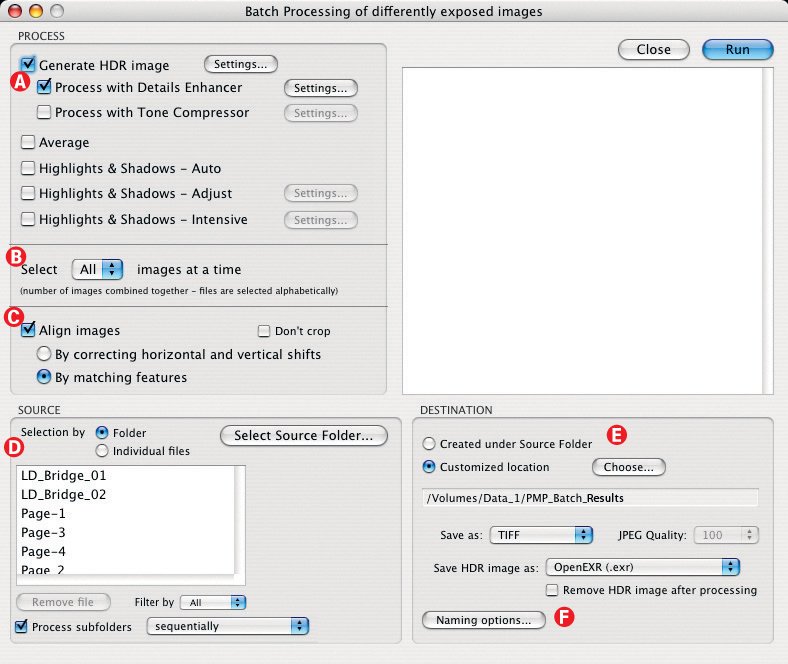
Figure 6-71: Almost all of the necessary batch processing settings can be found in this window.
![]() The settings to be used for aligning your source images. As before, By matching features is the best choice in most cases.
The settings to be used for aligning your source images. As before, By matching features is the best choice in most cases.
![]() The location of your source images, and the options for subfolder processing.
The location of your source images, and the options for subfolder processing.
![]() The location and output format for your results. You can also specify whether or not the intermediate HDR files should be deleted once processing is complete. As most of the important corrections take place at the tone mapping stage, it is advisable to keep the HDR images until you are satisfied with the final results.
The location and output format for your results. You can also specify whether or not the intermediate HDR files should be deleted once processing is complete. As most of the important corrections take place at the tone mapping stage, it is advisable to keep the HDR images until you are satisfied with the final results.
Finally, you can use the dialog ![]() to set a naming convention for your output image files. Photomatix Pro automatically attaches the letters “HDR” to HDR file names and appends “Compressor” or “Enhancer” to LDR file names, depending on which tone mapping method was applied. The exposure blending process also names outputs files “Average”, “Auto”, “Adjust_Fusion”, or “Intensive”, according to the method applied. In our example, the settings shown in figure 6-72 produced a satisfactory naming scheme, which allows us to easily refer back to our source images, regardless of where they are located.
to set a naming convention for your output image files. Photomatix Pro automatically attaches the letters “HDR” to HDR file names and appends “Compressor” or “Enhancer” to LDR file names, depending on which tone mapping method was applied. The exposure blending process also names outputs files “Average”, “Auto”, “Adjust_Fusion”, or “Intensive”, according to the method applied. In our example, the settings shown in figure 6-72 produced a satisfactory naming scheme, which allows us to easily refer back to our source images, regardless of where they are located.
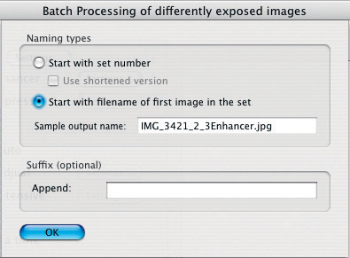
Figure 6-72: This dialog is used to set a naming convention for your output files.
You can define your HDR or tone mapping process more precisely using the Settings buttons ![]() (see also figure 6-71). These are the same settings that we already know from conventional HDR or tone mapping processes using Photomatix Pro, and you can use previously saved Preset configurations here too.
(see also figure 6-71). These are the same settings that we already know from conventional HDR or tone mapping processes using Photomatix Pro, and you can use previously saved Preset configurations here too.
Click Start to begin batch processing. Batch processes are run separately from the rest of the program, which means you can also perform other, non-batch Photomatix operations while your batch process is in progress.
The progress of the individual steps involved in the batch process are detailed during processing in the window shown in figure 6-73.
Finally – or as soon as the first results are ready – you can view your finished LDR images and optimize tone mapping in the appropriate HDR images if necessary. This is easier to do if you save your HDR and LDR images in their own folder, separate from your source images.

Figure 6-73: The Photomatix Pro batch processing window details the individual steps as they are carried out, and keeps you informed of progress.
Large batch processes can take time, but usually run without problems. We often use the Photomatix Pro batch process to make a “first draft” of our HDR images before further processing them using other HDRI tools.
Single File Conversion
A simplified batch processing function for single files can be found in the Automate menu under Single File Conversion. This process tone maps single HDR images located in a specific source folder and saves them as LDR images in a target folder. Here too, the user can specify the type of tone mapping to apply and the output format.
6.7 HDRI Using FDRTools
![]() FDRTools can be found at www.fdrtools.com. Help, discussion, and suggestions for further development of the program can be found in the FDRTools forum at: www.fdrtools.com/smf/index.php
FDRTools can be found at www.fdrtools.com. Help, discussion, and suggestions for further development of the program can be found in the FDRTools forum at: www.fdrtools.com/smf/index.php
You may ask yourself why we are presenting yet another HDRI tool, having already discussed Photoshop, PhotoAcute, and the very powerful Photomatix. The answer is, quite simply, because FDRTools offers functions which are not available in the other programs mentioned. Specifically, FDRTools offers increased control over the HDRI merging process, powerful tone mapping, and specialized viewing tools. FDRTools also includes a somewhat cumbersome, but nevertheless useful project management tool. Acquiring this software and learning how to use it effectively will definitely improve your general image processing skills.
![]() The 2.2 version of FDRTools Advanced also includes a focus stacking function (using the xDOF method). We will not be discussing this function at this point.
The 2.2 version of FDRTools Advanced also includes a focus stacking function (using the xDOF method). We will not be discussing this function at this point.
FDRTools’ functionality is comparable to that of Photomatix, and FDRTools Advanced has the distinct advantage of costing about half as much as Photomatix Pro. The free FDRTools Basic version also has more functionality than the free version of Photomatix. The program’s generally poor performance is constantly improving from release to release. FDRTools is available for both Windows and Mac OS X, and comes with detailed tool tips which make it fairly simple to use. Tool Tips are small text windows which temporarily display information about a particular tool if you move the mouse over the buttons or menus associated with it. According to the program’s creator, Andreas Schömann, a comprehensive user manual is currently being written.
We will use the abbreviations FDRT for FDRTools and FDRTA for FDRTools Advanced in the discussion that follows. FDRTA supports a number of source formats, including JPEG and TIFF, as well as the standard RAW and PNG formats. The program uses the Open Source dcraw RAW converter, and therefore recognizes all formats currently supported by dcraw. FDRTA can also be used to tone map HDR images created using other tools to LDR. As mentioned earlier in table 6-2 on page 153, other supported HDRI formats include 32-bit TIFF, OpenEXR, and Radiance.
The program’s user interface will probably appear somewhat unusal at first, as it consists of a number of different windows, not all of which are relevant to each phase of the process.
The program has two basic states – project management and image processing. When you start FDRTools, the first thing you see is the project management window (see figure 6-74). The project window will displays your current projects and can be used to start a new, empty project.
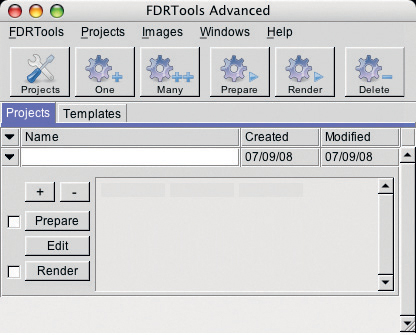
Figure 6-74: The FDRTools Start/Project window.
In order to work effectively with FDRTools, it’s necessary to grasp the concept of projects. A project in FDRTools is a set of data which encompasses references to the images involved and the operations and settings which are to be applied to them. The stored settings include alignment information, tone mapping type, and HDR merge type. Because FDRTA offers a number of different HDR merge process types as well as a number of different tone mapping methods, it remembers the last settings made for each type, whether they be the default settings or user-defined.
All of this information is saved in a project file and can be modified at any time, as long as you don’t explicitly delete the project. This type of project-based workflow plays no part in the Photoshop philosophy, and only exists in rudimentary form in Photomatix. This approach bears testimony to the fact that HDR images are often processed more than once, and that experimentation and subsequent reinterpretation are integral parts of the HDRI realm.
Project-based processing also allows you to revisit older image projects using newer versions of the program as they become available. Projects are saved in a designated directory, which you can select in the dialog that opens when you click the Project icon in the main window (see figure 6-75). In this same dialog box, you can also set a directory containing templates. Templates are, in principle, normal projects whose settings can be transferred to other projects.
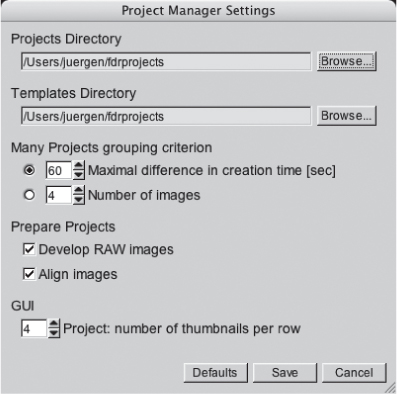
Figure 6-75: The FDRTA project management settings. These include the location of the project directory.
As with any other program, you want to customize FDRTools to suit your personal preferences once you have become familiar with it. The Preferences settings can be found under FDRTools ▸ Preferences. The online handbook will tell you more about the possibilities of each individual setting.
We now create a project by clicking the ![]() icon in the main window. The Open Images dialog box appears, which we use to select our source files. A filter shows us which files types can be selected, and these include LDR formats and HDR images created using FDRT or other tools. For images created using FDRT, you can also open your previously created images by opening the corresponding project. In our example, we will concentrate on creating an HDR image from a series of standard LDR image files.
icon in the main window. The Open Images dialog box appears, which we use to select our source files. A filter shows us which files types can be selected, and these include LDR formats and HDR images created using FDRT or other tools. For images created using FDRT, you can also open your previously created images by opening the corresponding project. In our example, we will concentrate on creating an HDR image from a series of standard LDR image files.
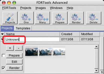
Figure 6-76: Naming your project.
The selected images appear as thumbnails in the project window. Give your project a suitable name by overwriting the Untitled label (see figure 6-76). At this stage, you can still add or remove images at any time. Click on the plus icon to navigate back to the Open Images dialog, or select an image and click the minus icon to remove it.
To delete an entire project, click anywhere in the project window (which is then highlighted) and click the Delete button in the tool bar above.
If you select an image and open its corresponding Exif window (Window ▸ Exif Info), you will be confronted with an unusually extensive Exif info listing. This can be useful when analyzing an image, and can be hidden if you don’t currently need it.
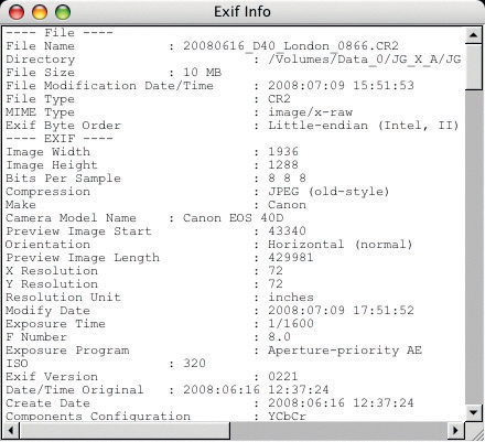
Figure 6-77: The FDRTA Exit’window. This illustration shows only a small portion of the data which is actually displayed in this window.
We recommend activating the progress window (in the Windows menu). This gives information (see figure 6-78) about the progress of currently active processes, and sometimes provides an explanation as to why FDRTools isn’t reacting as quickly as it might.
Figure 6-78: The progress window can also be a useful source of information.
The next step is to prepare your images – click the Prepare button in the project frame. If the project is already selected (i.e., highlighted), you can you can use the toolbar Prepare button, which also allows you to simultaneously prepare multiple projects using a batch processing function. Batch processing can take a while (see page 192 for more information), but once you’ve started the process, you can continue using your other tools while FDRTools is working.
The Prepare command prepares the images in a project for faster processing. Preparation itself can take some time, but makes the subsequent processes much quicker.
Once prepared, the individual images in a project are ready to be rendered. This means the actual HDRI generation process, or, in the case of existing HDR images, tone mapping.
Clicking Edit switches into a new view (see figures 6-79 and 6-80). The program window now shows a set of icons in the toolbar which reflect the workflow sequence of HDRI creation: Open, Alignment, HDRI Creation, Tone Mapping, and finally, Save. The yellow “lights” in the buttons signalize which phase of the process is currently active.
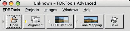
Figure 6-79: The FDRTA toolbar icons, shown in “Edit” mode. The buttons follow (from left to right) a typical HDRI workflow.
We have already described how to open images, and FDRTA usually aligns your images automatically during the preparation stage. The adjustments the program has made to alignment are listed next to each image in the program window. If this is not the case, click on Align in the Tripod tab. The Tripod alignment method is new since the release of the 2.0 version of the program, and other methods (such as Hand-held) are expected to be introduced in the near future.
You can correct image alignment manually (using the slider or by entering a value) if necessary, and you can check alignment in the Preview window, which displays images at a ratio of 1:1. The program aligns images relative to the first image in a project.
You can also temporarily deactivate images displayed in the list by clicking the Include button on or off. The green “light” in the button indicates that the image in question will be included in the pending process.
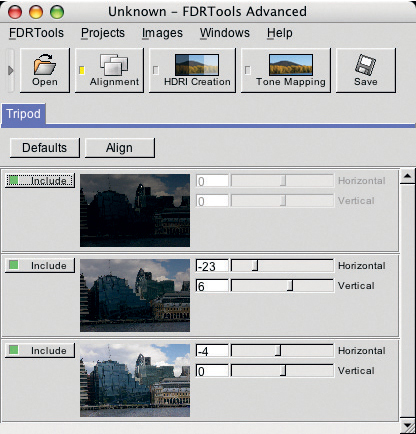
Figure 6-80: The basic window in its alignment mode.
One weakness in the current 2.2 (beta) version of FDRTA is its inability to align images using an object-based method. Photomatix Pro now includes this capability, which is a significant advantage.
The HDRI Creation Phase
In contrast to the other tools we have discussed, FDRTA allows us to control the HDRI generation process manually using a whole range of parameters. Clicking the HDRI Creation button displays the four merging methods available in the current (2.2) version of the program:
▸ Average
▸ Separation
▸ Creative
▸ xDOF
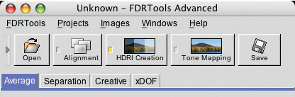
Figure 6-81: The “HDRI Creation” phase with the “Average” method activated.
The tool tips explain each process comprehensively. Each process uses its own algorithm, and uses sliders and curves to control the weighting of the individual source tones in the resulting HDR image. The histograms also help the user to visualize the merging process.
At this point, we already have a very broad range of parameters and settings at our disposal, and it is simply not practical to discuss them all individually. The best way to find out which parameters affect your images is to try them out.
But don’t panic! The program’s default settings usually produce perfectly acceptable results, and you will only usually need to intervene for difficult source material, or if you are not satisfied with the results the program produces.
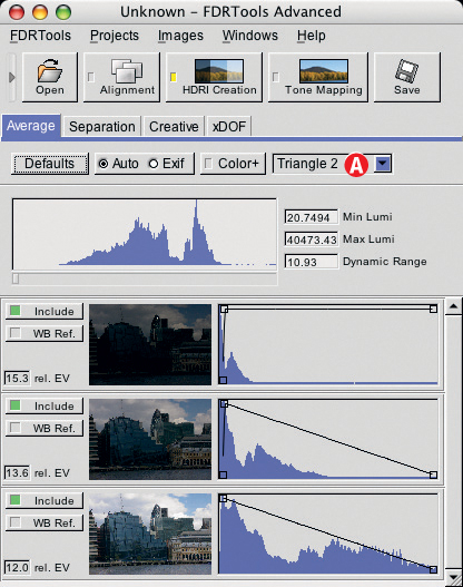
Figure 6-82: HDRI creation settings for the “Average” method.
Average
The Average method creates an HDR image based on the averaged tonal values of the pixels in the source images. The related curves (see 6-82) determine the exact weighting for each image. Various preset curves can be selected using menu ![]() , and you can make additional adjustments to these curves using your mouse, the same way as you can adjust a Photoshop Curve.
, and you can make additional adjustments to these curves using your mouse, the same way as you can adjust a Photoshop Curve.
The Average method requires additional image exposure information to function correctly, and it extracts this information from the file’s Exif data (if the source files are in RAW format). If no Exif data is available, the program attempts its own image analysis. You can switch between the two data extraction modes using the Auto/Exif button. The Color+ option produces strong color rendering in non-RAW images. This method can also be effectively used to generate reduced-noise LDR images from a series of source images taken with similar exposures.
Some of the merging methods provide a WB Ref. button in the image list, which allows you to select the image which should be used as a reference point for automatic white balancing. FDRTA will then attempt to adjust white balance for the remaining images accordingly.
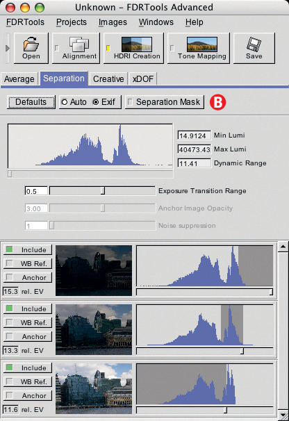
Figure 6-83: The settings for the “Separation” method.
Separation
When using the Separation merging method, each individual HDR pixel is taken from only one of the source images. Each image covers a particular area of tonal values (or intensity) which is determined by the program. Where two areas of differing intensity overlap, the program blends these pixels to provide a smooth transition. The slider beneath each histogram allows you to adjust the intensity, and with it the tonal values for each individual source image.
Separation also allows you a degree of control over moving objects via the Anchor option. Once you have selected an anchor image, FDRTA will search through all of your source images to identify any moving objects, replacing these portions of the image with corresponding pixels from the anchor image.
You can only select one anchor image, and this image should be one with regular, average exposure. The Anchor option was not yet fully implemented in our beta version of the program, which is why some of the buttons in the illustration are grayed out.
If you click Separation Mask (![]() ) and then one of the histograms, the non-red portion of the image then displayed in the navigator image or the tone-mapped preview window shows exactly which parts of that source image have been used in the resulting HDR image.
) and then one of the histograms, the non-red portion of the image then displayed in the navigator image or the tone-mapped preview window shows exactly which parts of that source image have been used in the resulting HDR image.
Creative
As the name suggests, this is the most flexible merging method offered by FDRT. According to the program’s author, it can be used to merge images with very different, almost arbitrary exposures (for instance, an object lit using multiple light sources) to create interesting and unexpected effects.
The three options Intensity, Saturation, and Contrast (![]() ) allow you to set the selection criteria for the pixels which are to be taken from each source image. The menus
) allow you to set the selection criteria for the pixels which are to be taken from each source image. The menus ![]() and
and ![]() allow you to select differing curve weighting presets and to switch between Linear and Logarithmic layer scaling.
allow you to select differing curve weighting presets and to switch between Linear and Logarithmic layer scaling.
It is also possible to edit the individual curves manually using the mouse, allowing you to determine precisely the weighting the merging process gives to each individual image area.
This method is very powerful, but also makes it relatively easy to get bogged down when experimenting with different combinations of settings. We therefore only recommend using this method if you are not satisfied with the results you achieve using other methods.
While the preview window helps to preserve an overview of the changes you are making, the program is still entirely lacking a Save feature for saving combinations of settings for later use, either for the same image or for other projects.
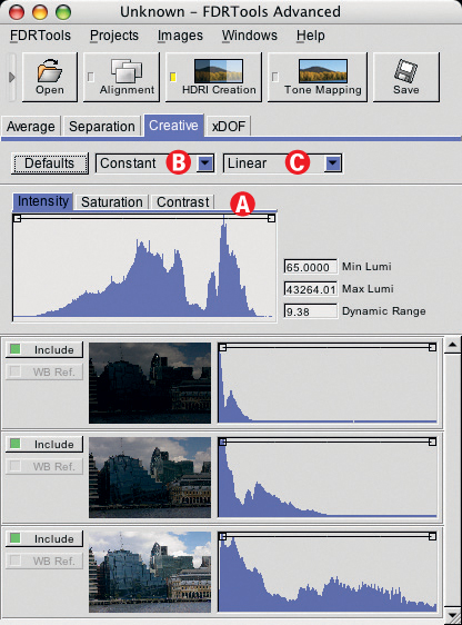
Figure 6-84: The “Creative” merging method offers the most individual settings.
xDOF
The unusual name of this merging method stands for Extended Depth of Field, and was introduced in the 2.2 version of the program. It is still under development (or was, in the beta version we were using at the time of writing). The process aims to create an HDR image while simultaneously applying a focus-stacking technique. Focus stacking merges source images with varying depths of field into a single image with extended depth of field. The technique is described extensively in chapter 4.
Because FDRTA’s alignment and scaling processes are not yet as advanced as those of Helicon Focus or MergeZM, we will not go into any further detail here.
Should you over-adjust a parameter – which can happen at any stage of the process – a click on the Defaults button resets the program to its standard settings. The button is available at the Alignment, HDRI Creation, and Tone Mapping stages.
FDRTA updates the preview image and the HDRI histogram for every change you make to a process or parameter, helping you to judge the effects of your changes accurately. FDRTA also displays the total dynamic range and maximum and minimum luminance values for each image, making it especially easy to determine which method delivers the best dynamic range for your particular subject (see figure 6-86).
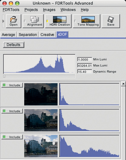
Figure 6-85: The “xDOF” merging method is new and has, as yet, no user-controllable parameters.

Figure 6-86: FDRTA updates the histogram and luminance values after every change of settings.
Now we have described the program in theory, we will apply it to two very different image sequences. The first was shot hand-held in London, and you will recognize it from earlier examples. The original images were straightened and cropped using a RAW converter before being saved as the 16-bit TIFF source files shown in Figure 6-87.
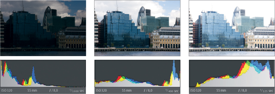
Figure 6-87: The source images were shot bracketed and hand-held. They were straightened using a RAW converter and saved as 16-bit TIFF files.
Figure 6-88 shows the results of applying the three different HDRI Creation methods available in FDRTA* displayed in the Tone Mapped Image tab of the navigator window. These HDR variations were all generated using the default program parameters and without any additional optimization. We used the image generated by the Separation method as the base image for our tone mapping experiments, although the provisional nature of the preview image makes it difficult to judge exactly which image displays the best characteristics.
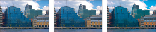
Figure 6-88: HDRI results (tone mapped preview images in the program’s navigator window) as generated from the sequence shown above. Left: “Average”, Center: “Separation”, Right: “Creative”.
Our second sequence (see figure 6-89) was shot at sunrise in Page, Utah. We worked with relatively long exposure times, as the exposure data shows. We used a tripod, a cable-release, and mirror lock-up. Due to the long exposure times, the smoke coming out of the power plant’s smokestacks has become a moving object. The middle exposure shows how low the actual dynamic range in the scene was, and we could have worked with smaller bracketing steps to help minimize noise.
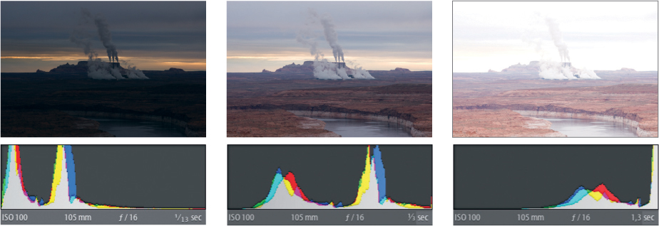
Figure 6-89: Our three source images with exposure information and histograms. The bracketing increment was set to 2.0 EV.
Figure 6-91 shows the results of the first three HDRI creation runs, again using the default parameters and the Tone Mapped Image tab in the navigator window. The Separation result was our favorite, and we used this as the base image for our tone mapping.
There are some coverage problems where the smoke rises past the bright cloud (figure 6-90), and some clone stamp work is necessary before printing. The next version of FDRTA, with its Anchor function will help to alleviate such problems. The function was not yet implemented in our beta version, so there were no real recognizable differences between the results produced by all three merging methods.
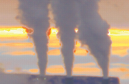
Figure 6-90: Some artifacts are visible where the smoke and the sun cross Paths.
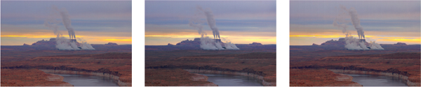
Figure 6-91: The results of three HDRI merging methods. Left: “Average”, Center: “Separation”, Right: “Creative”.
Saving Your HDR Files
It is never a disadvantage to save each HDR image along the way. Click the HDR Image Inspector tab in the navigator window to make sure the HDR image is active, then click the Save button in the main window to open the Save dialog.
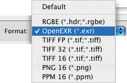
Figure 6-92: The HDR output formats offered by FDRTA Version 2.2.
FDRTA offers multiple HDR formats, most of which also offer several compression options. You will need to experiment a little to find out which combinations are supported by the other HDR tools you use. We recommend using Radiance or OpenEXR formats. If you can only see LDR formats in the Save dialog box, this a sign that the LDR image rather than the HDR image is active in the preview window.
You can also set the program to automatically open your HDR image in another program. This can be useful if you plan to crop, align, or otherwise correct your image (using Photoshop, for example) before you start the tone mapping process. You will, however, have to explicitly open your image in an FDRTools project in order to proceed with tone mapping. We have noticed that Photoshop displays HDR files (or, at least, OpenEXR files) much brighter than FDRTools does. We had to move the Photoshop 32-bit white point slider almost all the way to the left in order to be able to see any detail in an HDR file which appeared quite dark in FDRTools.*
The FDRTools “Tone Mapping” Phase
Evaluating the HDR preview image accurately can be difficult, as the image displayed is only provisionally tone-mapped. Once you have (optionally) saved your HDR image, you can start the most interesting phase of the process by clicking the Tone Mapping button. The HDR Image Inspector and Tone Mapped Image navigator windows were certainly useful for aligning our source images and generating the HDR images. For this part of the process, they are absolutely indispensable.
FDRTA offers three tone mapping methods: Simplex, Receptor, and Compressor. While the Simplex and Receptor methods apply a global tone mapping to your image, the Compressor method performs an additional local tonal value adjustment which takes the pixels surrounding each individual pixel into account. This makes Compressor the most processor-intensive and time-consuming of the three methods.
In order to view your results more precisely, you can use the Window menu to activate the Preview option, which displays an image detail at 100% magnification in a separate window. You can move the location of the detail within the preview window either by using the scroll bars in the window itself, or by moving the detail frame in the navigator window using your mouse. The preview window can be enlarged, but making it too big can cause the program’s performance to suffer.
“Simplex” Tone Mapping
This method is designed to give the user quick and effective results. It offers two adjustable parameters: the Saturation slider and the gradation curve, which we use to set the white and black points. As with the Photoshop Local Adaptation method and the Photomatix processing dialog, there is no warning in the preview image to alert us to potential clipping situations. This makes it all too easy to clip highlight detail without the difference being visible in the histogram display – a problem which also applies to the Receptor and Compressor tone mapping methods.* The Simplex method uses a basis gradation curve and the editable curve superimposed upon it to reduce the dynamic range of your HDR image to that of an LDR image.
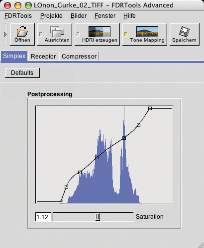
Figure 6-93: Simplex tone mapping is a global method, offering only one slider and a gradation curve for manipulation.
Figures 6-94 and 6-95 show two images created using the Simplex tone mapping method and their related settings. We were not satisfied with either result, but nor were we with the results Photoshop produced. These kinds of results are always strongly influenced by the subject matter and the distribution of tonal values that was originally captured.
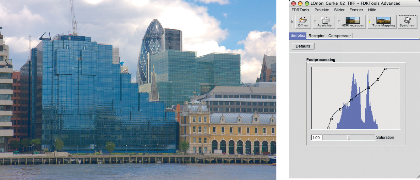
Figure 6-94: Simplex tone mapping clipped some of the detail in the clouds and darkened the shadows too much.

Figure 6-95: A Simplex-generated LDR image of the Page Power Station created using the settings shown on the right.
“Receptor” Tone Mapping
According to the program’s author, this method is one of the most advanced global tone mapping techniques available. Like the Simplex method, Receptor is based on the use of a gradation curves base, but is much more adaptable, and functions in a similar way to the Photoshop Highlight Compression tone mapping method. Receptor compresses the highlights more strongly than the shadows, which preserves highlight detail – a desired effect in most cases. Unlike the Photoshop solution, Receptor offers Compression, Brightness, and Saturation adjustment sliders, as well as the gradation curve, which you can use to adjust the black and white points. The Compression slider controls the degree to which highlight areas are compressed and is applied almost exclusively to the upper third of the tonal range. Brightness, too, applies mainly to the higher tonal values and has almost no effect on image shadows. Saturation functions the same way as it does for the Simplex method.
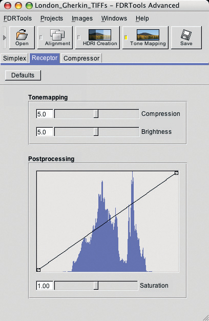
Figure 6-96: The “Receptor” process primarily compresses highlights.
Figures 6-97 and 6-98 show the results of tone mapping our two images using the Receptor method. The London image didn’t turn out very well, and we were not able to portray the clouds satisfactorily – and they were the reason we shot our HDRI bracketing sequence in the first place. Increasing compression didn’t help, and the mid-tones are simply bland. We had to use very steep curves in the upper and lower ranges to achieve a reasonable degree of detail in the highlights and shadows.
Our image of the Page power station, however, turned out better, due to the generally narrower tonal range involved. Receptor hasn’t produced perfect results, but they are certainly acceptable.
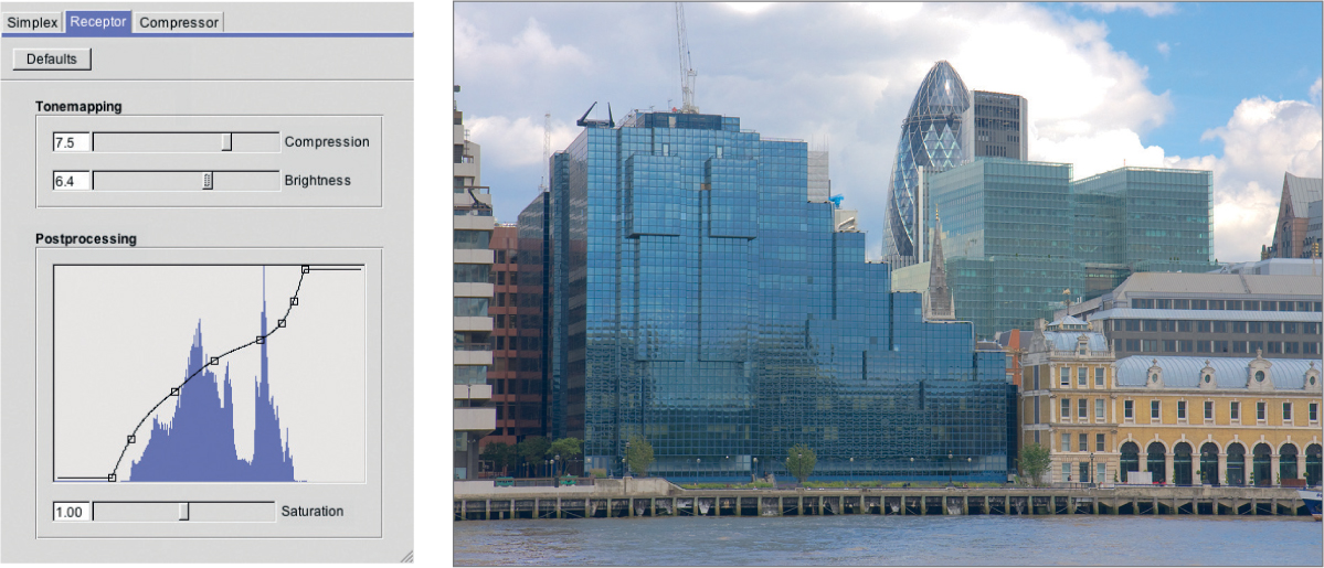
Figure 6-97: Our Thames view in London, tone-mapped using the “Receptor” method.
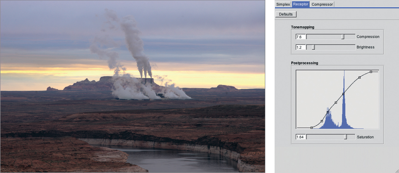
Figure 6-98: An LDR version of our power station image, created using the “Receptor” tone mapping method.
We really wanted more texture in the clouds, but we were not able to achieve this using Receptor, in spite of several attempts at fine-tuning the curve. We were also not able to brighten the darker foreground sections of the image. One solution to this problem would be to go back to the HDRI generation stage and use Creative mode to reduce the weighting for the darker areas in the final, composite image. Creative mode offers a great deal of flexibility, but using it effectively can be time-consuming.
“Compressor” Tone Mapping
This method is the FDRTA equivalent to Photoshop’s Local Adaptation and Photomatix Pro’s Details Enhancer, and produces the best results of all. The process uses a gradation curve combined with a step that analyzes each pixel and the tonal values surrounding it individually. This process uses large amounts of processing power and is therefore also slower than FDRT’s other methods.
Here too, the Compression settings determines the degree to which source image ares are compressed in the final image, but this time only in relation to the immediate surroundings of each pixel. Contrast governs microcontrast, with moderate values producing softer transitions between image areas. Higher contrast values result in a typical, high-contrast HDR look. The Smoothing slider functions as a kind of microcontrast multiplier – the higher the value, the softer and more natural the transitions and edges in your image will be. An image with a high dynamic range will always need more smoothing than one with a moderate dynamic range.
The 360° Panorama option is only useful for ensuring a smooth merge where the ends of a 360° panorama sequence meet.
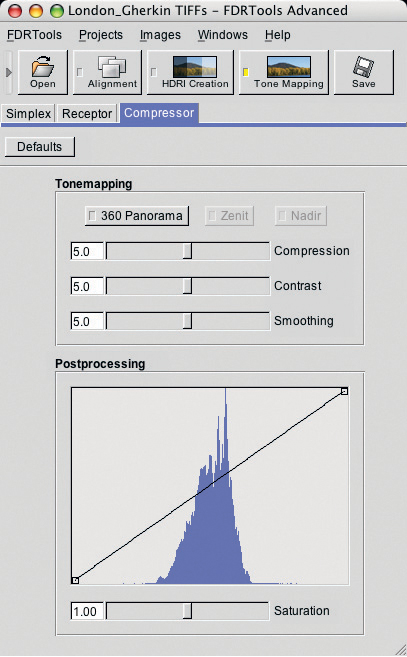
Figure 6-99: The “Compressor” tone mapping process.
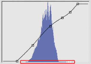
Figure 6-100: To avoid clipping, make sure you preserve low peaks to the left and the right of the histogram.
Figure 6-101 shows our London image, tone-mapped using the Compressor method. This method’s multiple settings make it possible to produce more individual image interpretations than the other methods allow. This version of our image looks much better, and we have finally managed to preserve our cloud detail, but at the price of a strong, high-contrast HDRI look. A glance at the histogram confirms that all of the shadow detail and – more importantly – highlight detail has remained intact (see figure 6-100).
For lifeless-looking images, we have found it effective to leave a little leeway at the left and right ends of the histogram, and then to save the image to 16-bit TIFF before optimizing the colors (and setting black and white points) using a Photoshop Levels adjustment layer. Alternative scaling methods would make optimizing the curve easier, but this feature is unfortunately not (yet) available in FDRTools.
One way to avoid a heavy HDRI look would be to create two image versions: one with pronounced cloud detail, and the other with generally less contrast, especially in and around the buildings. We could then use Photoshop layers and layer masks to blend these two images together using the techniques we have already discussed. As with most images that result from merging processes, the image shown in figure 6-101 could benefit from a little post-processing.
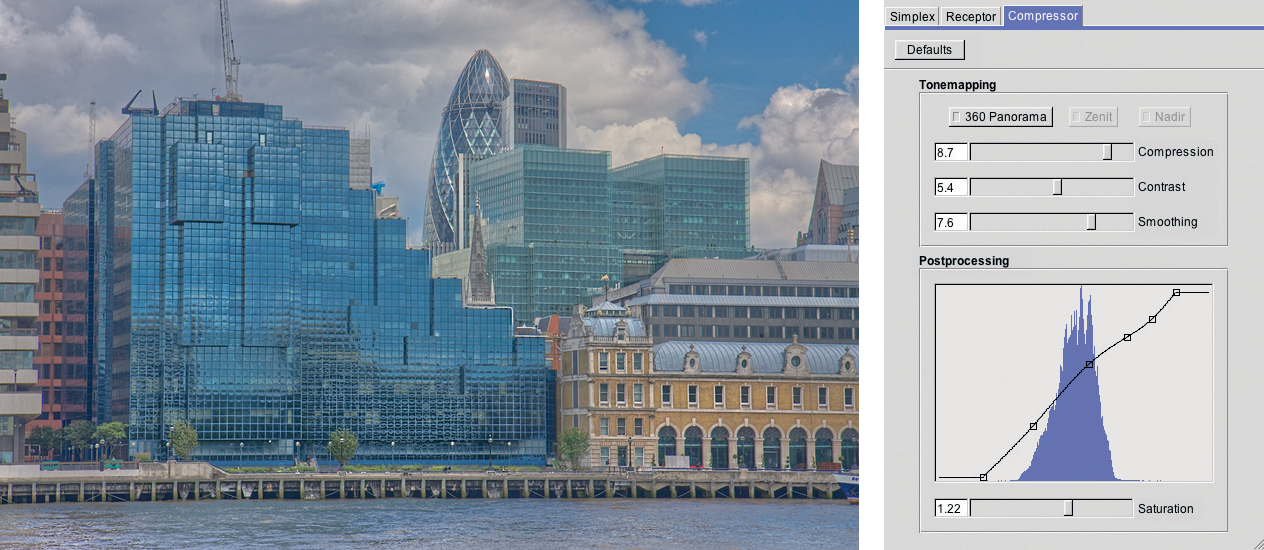
Figure 6-101: The result of using “Compressor” tone mapping and the settings shown to the right. This time, cloud detail was not clipped, but the mid-tones have turned out somewhat flat, and can benefit from some post-processing.
We post-processed our image using Photoshop, and the Layers palette in figure 6-99 shows the steps we took. We duplicated the background layer and used Filter ▸ Distort ▸ Lens Correction to soften pin-cushion distortion and to correct slight horizontal and vertical perspective anomalies. We then used the Levels command on a second layer to increase global contrast and brighten the image slightly, which also increased color saturation a little.
Our master image is now finished, and can be saved and used as a basis for further fine-tuning experiments.
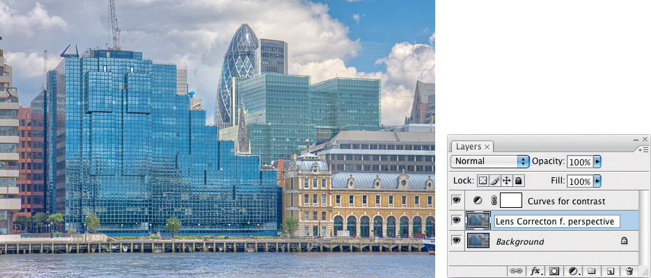
Figure 6-102: The final version of the image shown in figure 6-101 and the Layers palette for the post-processing steps we applied to it.
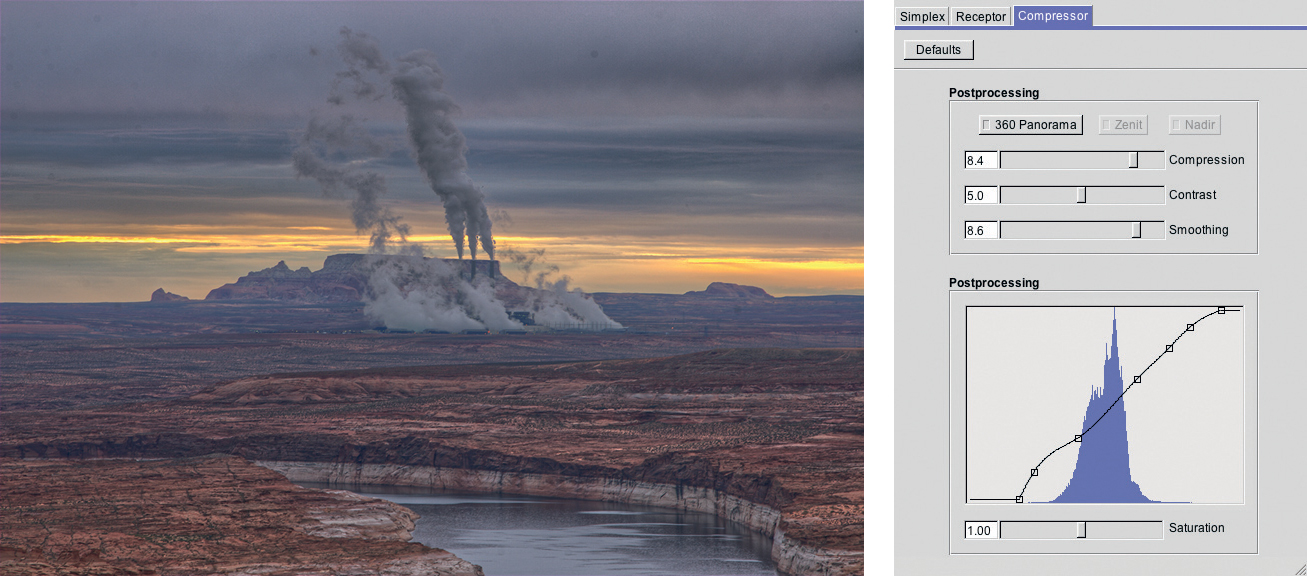
Figure 6-103: The LDR result of a “Compressor” tone mapping using the settings shown on the left.
Figure 6-103 shows our power station image after tone mapping using the Compressor method. The image was taken at sunrise but doesn’t really contain the colors we remember. We therefore tried to adjust white balance using the eyedropper tool from the FDRTools toolbox (figure 6-104). To do this, we select the eyedropper tool and click in an area of the image that should appear neutral gray once the correction is done – this is technique you may already be familiar with from your work with the Photoshop Levels command. You can always adjust your settings using the Red Balance and Blue Balance sliders if your first attempt doesn’t deliver the desired result.
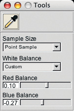
Figure 6-104: You can adjust the white balance of an HDR image using the eyedropper tool and the corresponding sliders.
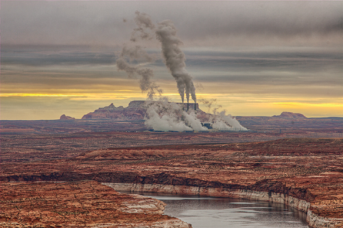
Figure 6-105: Our image after white balance correction using the eyedropper tool.
(The White Balance dropdown menu allows you to return to the original image settings by selecting As Shot.) In our example, we used the whitish-gray smoke as our neutral reference point and increased saturation to achieve the result seen in figure 6-105. The image is now much more reminiscent of a sunrise, and even shows a slightly brighter foreground. The image has a slightly surreal look, but this is an accurate representation of the early-morning scene we photographed, with a light mist still covering the valley floor.
Saving LDR Images
The final step of the FDRTools workflow is to save the resulting tone-mapped image in to an LDR format. As before, click the Save button, and make sure you are saving the LDR and not the HDR image. If you want to continue editing your image using Photoshop (or any other similar program), we recommend that you save your image to the usual 16-bit TIFF format. The color space you choose for your LDR files also plays a role, but this setting can only be changed using the Output Device option in the Devices tab of the program’s Preferences dialog. We would prefer to see this setting as part of the Save dialog.

Figure 6-106: FDRTools can save to a number of different LDR formats.
We opened our image directly in Photoshop from the FDRTools Save dialog. We adjusted the levels and then increased the contrast in the sky using the Curves adjustment layer. We also used the Clone Stamp tool (![]() ) to remove some spots that resulted from flecks of dust on the camera’s sensor, and we also removed the artifacts we mentioned previously that occurred where the rising smoke passes through the sunlight. Finally, we sharpened our image a little (using Filter ▸ Sharpen ▸ Smart Sharpen), using a layer mask to protect the sky. The final result can be seen in figure 6-107.
) to remove some spots that resulted from flecks of dust on the camera’s sensor, and we also removed the artifacts we mentioned previously that occurred where the rising smoke passes through the sunlight. Finally, we sharpened our image a little (using Filter ▸ Sharpen ▸ Smart Sharpen), using a layer mask to protect the sky. The final result can be seen in figure 6-107.
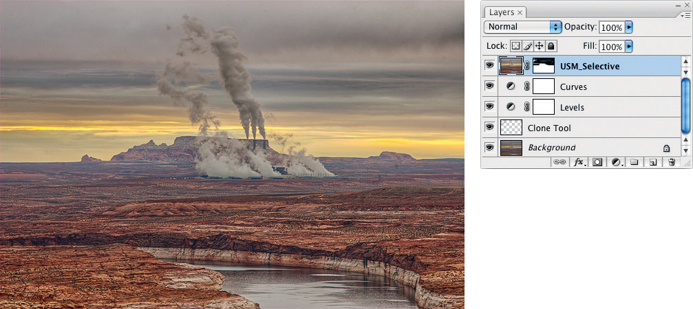
Figure 6-107: The image after Photoshop post-processing.
Some Observations
None of these three tone mapping processes can correlate the luminance of a particular pixel in the HDR image to a point on the gradation curve – a feature already included in Photoshop. Including this functionality would make editing a gradation curve in FDRTools simpler and much more intuitive.
After we initially spent a lot of time and effort attempting to perfect the gradation curve, we have now adopted a different workflow. Now, we simply fix an approximate gradation curve, leaving some processing leeway at the right and left ends of the histogram. We then save the LDR file to 16-bit TIFF and open the resulting file directly in Photoshop, where we use a Levels adjustment layer and a Curves adjustment layer to optimize our tonal values. As of Photoshop CS3, both of these adjustments are now handled by the Curves dialog – the histogram is now displayed in the curves window.
Back to the Project Window
You can switch easily between the program’s individual functions by clicking on the appropriate buttons in the toolbar. You can save the current state of your work at any time using the menu sequence Project ▸ Save active. We highly recommend saving your work at regular intervals, just in case the program crashes. This has happened to us on a number of occasions.* If you want to return to the main program window, you can use the menu sequence Project ▸ Close active at any time.
Batch Processing
FDRTools Advanced offers a function that is very similar to traditional batch processing. This multi-project functionality works as follows:
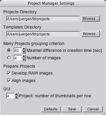
Figure 6-110: FDRT’s major project management settings.
1. Start by defining the source images for your projects and selecting a template. To create a new template, activate the Templates tab, create a new project and make the settings you want to use. These settings will now also be available as a template.
If you use the Many button (rather than the One button), you can select the criteria the program uses to group your source images into projects – the maximum allowable time lapse between shots, or the number of images per project, for instance. You can select these criteria in the dialog displayed (see figure 6-110) when you click the Projects button ![]() .
.
2. Now select the project you wish to process, and check the appropriate processing options (Prepare or Render).
3. Click the Prepare button ![]() at the top of the project window, and confirm the security query that follows. All of your projects will now be prepared for fast processing.
at the top of the project window, and confirm the security query that follows. All of your projects will now be prepared for fast processing.
4. The final step (it is also possible to simply skip step 3) is to click the Render button ![]() in the toolbar. This will start the conversion of all of your projects into HDR images, which will then be converted into LDR images and saved in the project folder. You can select which HDR and LDR formats you want to use using the Output Device tab in the FDRTools ▸ Preferences menu.
in the toolbar. This will start the conversion of all of your projects into HDR images, which will then be converted into LDR images and saved in the project folder. You can select which HDR and LDR formats you want to use using the Output Device tab in the FDRTools ▸ Preferences menu.
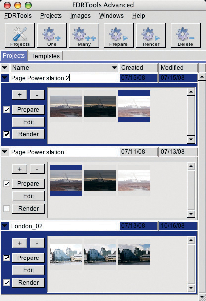
Figure 6-108: The project window with two projects selected.
As a final procedure, you should check the quality of your LDR images. If any corrections are necessary, open the project in question, activate Edit mode, and correct your HDR image either by changing the parameters for the HDRI creation process or for the Tone Mapping process.
FDRTools – Our Conclusions
We had some difficulty getting used to the program’s concepts and workflow, and some of its processes are definitely slower than their counterparts in some of the other tools we have discussed. As with most complex tools, the longer you work with FDRTools, the more you will become familiar with the many possibilities it offers, and the faster you will be able to achieve satisfactory results. FDRTools is under constant development, and represents great value when you consider the price, the performance and features it offers.
We have only discussed a relatively narrow spectrum of the possibilities and variations the program offers. You can often combine the various functions to achieve better results – you could, for instance, merge a series of high-noise night shots to a low-noise LDR image using the Average HDR process, and then merge the resulting LDR image with a lower-noise shot of the same scene taken using a shorter shutter speed. The end result would then be an HDR image with significantly reduced noise. Noise is one of the problems inherent in HDR images, and local mapping techniques often visibly increase the intensity of the problem.
![]() Here, I have a request for the program’s author: It would be great to be able to really close a project (so that it disappears from the project list) and then use a “Load” function to reload it into the list later.
Here, I have a request for the program’s author: It would be great to be able to really close a project (so that it disappears from the project list) and then use a “Load” function to reload it into the list later.
One work-around for the program’s somewhat weak alignment functionality is to load your source images into Photoshop as a stack, align and crop them, and then export them as separate LDR images. As of the CS3 version, Photoshop can export aligned images from individual layers into separate files using the menu sequence: File ▸ Scripts ▸ Export Layers to Files.
You can then load these into FDRTools in the normal fashion and convert them to HDR using an appropriate method before carrying out any tone mapping. PhotoAcute also offers alignment and re-export functionality.
6.8 Which Program Is the “Right” One?
As you might expect, the answer to this question is: “That depends.” Each of the programs and each method we have looked at has its own particular advantages and disadvantages.
The Photoshop blending technique appears at first to be quite sparse, but can be used in a number of ways. It also uses only limited resources, and doesn’t require any additional programs or plug-ins. The process does not require any specialized tone mapping, and it is often impossible to detect that the results have been processed using DRI techniques. The downside of this simple Photoshop approach (which is quite separate from the Photoshop HDRI function) is that, without complex post-processing, the results can only ever encompass a relatively narrow dynamic range.
In most cases, the same applies to PhotoAcute. One advantage of using PhotoAcute is that you can combine multiple corrections and apply them all in one processing run. You can, for example, simultaneously correct lens distortions (if a PhotoAcute profile for your camera/lens combination is available), reduce noise, and increase image resolution (provided multiple source images are available). Tone mapping parameters in PhotoAcute are not user-variable, and the program’s output is limited to 8-bit or 16-bit images, rather than the 32-bit output that Photoshop, FDRTools, or Photomatix Pro can produce.
Photomatix is a faster program with multiple capabilities and customizable tone mapping. The 3.02 version (which we used) was the best program for handling moving objects, but nevertheless encountered problems with objects that moved significantly during the shooting sequence. The download version isn’t exactly cheap (at around $90*), but we think it represents good value for the money. The program enjoys rapid development, and is updated several times a year.
FDRTools is traditionally very slow, and while it’s true that none of these programs can generate HDR images very quickly, FDRTools always had the additional problem of also reacting slowly during the loading and preparation phases. As of version 2.2 (we tested the beta version), this situation has improved a great deal.
Photomatix’s great strength lies in the very powerful Details Enhancer tone mapper and its batch processing functionality. FDRTools Advanced, on the other hand, offers great flexibility with regard to user control for the HDRI generation process. The Compressor tone mapping method also produces great results, although it tends also to produce unwanted noise. The FDRTools project management system is very useful, and the program’s greatest weakness lies in its limited ability to align images.
The grunge look which dominates many HDRI images raises questions of personal taste. We find that extreme-looking images quickly become boring. We prefer images which have a more natural appearance, even if this means accepting an image with less local contrast. At the end of the day, the processing steps that are applied to an image remain the photographer’s own decision.
You will also often find that one combination of HDR settings will work well for one particular image area (to accentuate a dramatic sky, for example), while a different combination works better for another part of the image. In such situations, we recommend that you create multiple copies of your image and use the Photoshop layer and layer mask techniques we have described to merge individually optimized sections of the image for a complete result.
Gaining Experience through Experimentation
All of the programs and processes we have described require a great deal of experimentation on the part of the user. You will need to develop a feel for the tone mapping process that works best for certain types of images, and – especially for images with a high dynamic range – you will need to develop your own style, which can also be heavily influenced by the subject matter and the type of output you want to produce.
We have mentioned many times that it is important to save intermediate results. HDRI generation is an inherently unstable process, and all four programs mentioned are subject to hangs or crashes. FDRTools crashed a little more often than the other programs, but we attribute this to our test version being a beta version.
Moving objects are the bane of HDRI images, and although each of the programs we have mentioned offers its own solution to the problem, none of them are really ideal. The best way to avoid this particular problem is to take care while shooting – avoid excessive wind, too much traffic, or too many pedestrians, and try to keep your sequences short.
Figure 6-109 shows an image that we created using three source photos shot using a tripod and a remote release. The exposure times ranged from 0.1 to 0.6 seconds,* and the ISO speed was set to 400. We used FDRTools Advanced and the Creative method to create the merged HDR image. Finally, we used Compressor for tone mapping to get the LDR version. We also slightly cropped the final image and applied DOP Detail Extractor to enhance the local contrast.
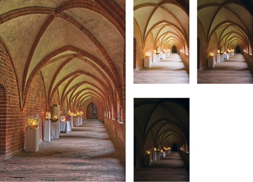
Figure 6-109: Our three source images and the resulting image, created using FDRTools 2.2, “Creative” for HDR generation and “Compressor” for tone mapping.
Post-Processing
Most LDR images that are created from HDR images will require some post-processing. As we have mentioned a number of times, there are certain optimization steps that cannot be applied directly to HDR images. These steps will include fine-tuning, cropping, and sharpening. If you use RAW files as HDRI source images, you may also need to correct aberrations in your LDR images. You will often find that small errors are difficult to detect in the HDR preview and therefore have to be corrected in the resulting LDR image. We have mentioned many post-processing ideas in the course of this chapter – you will find further, in-depth discussion on the subject in chapter 7.