6 Key-value Stores and Document Databases

This chapter covers key-value stores and document databases. Key-value stores are specialized for the efficient storage of simple key-value pairs. Parallel processing of key-value pairs has been popularized with the Map-Reduce paradigm. The Java Script Object Notation (JSON) is a textual format of nested key-value pairs. Document databases use JSON as their main data format. Last but not least, JSON is often used as a format for payload data in REST-based APIs.

6.1 Key-Value Storage

A key-value pair is a tuple of two strings [angbracketleft]key, value[angbracketright]. A key-value store stores such key-value pairs. The key is the identifier and has to be unique. You can retrieve a value from the store by simply specifying the key; and you can delete a key-value pair by specifying the key. A key-value store is the prototype of a schemaless database system: you can put arbitrary key-value pairs into the store and no restrictions are enforced on the format or structure of the value; that is, the value string is never interpreted or modified by the key-value store. Hence, a key-value store basically only offers three operations: writing (“putting”) a key-value pair into the store, reading (“getting”) a value from the store for a given key, and deleting a key-value pair for a given key.

store.put(key, value)

QueryResult queryResult =value = store.get(key)

store.delete(key)

With this simple interface, values cannot be searched and there is no advanced query language; if a combination or aggregation of several key-value pairs is needed, the accessing application is responsible or combining the corresponding key-value pairs into more complex objects.

The characteristic feature of a key-value store is that it is “simple but quick”: Data are stored in a simple key-value structure and the key-value store is ignorant of the content of the value part.

An advantage of this simple format is that data can easily be distributed among several database servers; hence, key-value stores are good for “data-intensive” applications. Typical applications for key-value stores are session management (where the session ID is the unique key) or shopping carts (where the user ID is the key). A generic application for the key-value pair data format is the map-reduce framework discussed in the next section.

In practice, in most key-value stores, values are allowed to have other data types than just strings. For example, a value can be a collection like a list or an array of atomic values; they support advanced search and indexing features. Some key-value stores also support data formats like XML or JSON – and hence are very close to document databases (see Section 6.2).

6.1.1 Map-Reduce

Under the name “map-reduce” a framework has come to be known that greatly simplifies the distributed processing of data in key-value format.

The basic elements of map-reduce are four functions that operate on key-value pairs (or on key-value pairs where the value is actually a list of values): split, map, shuffle and reduce.

While split and shuffle are more or less generic functions that can have the same implementation for all applications, the other two – map and reduce – are highly application-dependent and have to be implemented by the user of the map-reduce framework. Map and reduce are executed by several worker processes running on several servers; one of the workers is the master who assigns new map or reduce tasks to idle workers. Roughly, the four basic steps proceed as follows:

1.split input key-value pairs into disjunct subsets and assign each subset to a worker process;

2.let workers compute the map function on each of its input splits that outputs intermediate key-value pairs;

3.group all intermediate values by key and assign (that is, shuffle) each group to a worker;

4.reduce values of each group (usually one key-value pair for each group) and return the result.

A typical illustrative example for a map-reduce application is counting occurrences of words in a document (see Figure 6.1). The input is a document consisting of several sentences; counting the words consists of four steps:

1.the split function splits the document into sentences; each sentence is assigned to a worker process;

2.the worker thread starts a map function for each sentence; it parses a sentence and for each word word_i, the worker thread emits a key-value pair (word_i, 1) that denotes that the worker has encountered word_i once; these intermediate results are stored locally on the worker’s machine;

3.during the shuffle phase, local intermediate results are read and grouped by words; the 1-values for each word are concatenated into a list: that is, for each word there is a key-value pair where the word word_i is the key and the value is a list of 1s corresponding to individual occurrences of the word in all sentences: (word_i, (1, …, 1)) then, each word is assigned to a worker process;

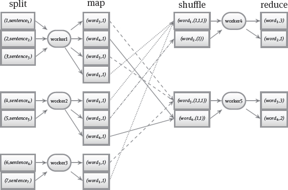
4.the worker thread starts a reduce function for each word that calculates the total number of occurrences by summing the 1s; as the final results it outputs the key-value pair (word_i, sum_i).

More formally, the signatures for the four functions can be defined as follows: –

–split: input ! list(key₁, value₁); that is, split maps some input text to a list of key-value pairs – for example, to a list where the sentence number is the key and the sentence content is the value.

–map: (key₁, value₁) ! list(key₂, value₂); that is, map processes one key-value pair and maps it to a list of key-value pairs; the new key key₂ (for example, the word word_i) usually differs from the old key key₁ (for example, the sentence number).

–shuffle: list(key₂, value₂) ! (key₂, list(value₂)); that is, shuffle groups the individual key-value pairs by key and appends to each key a list that is a concatenation of the values of the individual pairs.

–reduce: (key₂, list(value₂)) ! (key₃, value₃); that is, reduce aggregates a list of values into a single one; the keys key₂ and key₃ can be identical (as for example, word_i) and value₃ is calculated from the list of values list(value₂) (in our example, by summation).

Lastly, we highlight some features and optimizations of the basic map-reduce setting:

Parallelization: What makes map-reduce a good fit for processing large data sets is that the map as well as the reduce task can be run in parallel by different concurrent worker processes and even on multiple servers. This can be done as long as all map and reduce task are totally independent of one another; in our example, a map process can be executed on a sentence without requiring any input from any other map process. It is crucial to have a master process to coordinate the parallelization. The master keeps track of worker processes and it assigns map and reduce processes to idle workers. The master must also handle failures of worker processes: the master checks on a regular basis if a worker process is still alive; if a worker does not respond to this check, the master has to assign the process running on the failed worker to another one. If the failed process was a map task, the master must notify reduce task that want to read the output from the failed worker of the new location of the map task.

Partitioning: Usually, there are more reduce tasks to be executed than workers available. That is, each worker has to execute several reduce task on a set of different keys key₂. In our example, several different words will be mapped to a worker to execute the reduce task for each word. The subset of keys assigned to the same worker is called a partition. A good default partitioning can be achieved by using a hash function on the keys (which results in a number for each key) and then using the modulo function to obtain the number of a worker. In other words, if we have R workers that can accept reduce tasks, then for each key we can compute hash(key) mod R: the hash function maps the key to a number and mod splits the key space into R partitions called buckets. The user can influence the partitioning by specifying a customized partitioning function.

Combination: Instead of locally storing lots of intermediate results of the map processes which later on have to be shuffled to other workers over the network, an additional combine task can be run locally on each worker after the map phase. This combine function is similar to the reduce function as it groups the intermediate results by key and combines their values. Hence, we have less intermediate results that have to be shuffled. In our example, the combine task can even be identical to the reduce task and results in intermediate word counts for each worker (see Figure 6.2).

Data Locality: Transmitting data to a worker over the network is costly. To avoid overabundant transmissions, the master can take the location of data into account before assigning a task to a worker. For example, if a server already has copies of some sentences, map tasks for these sentences should be assigned to a worker on the same server.

Incremental Map-Reduce: Input data might be generated dynamically over a longer period of time. To improve evaluation of such data, the four steps can be interleaved and final results be obtained incrementally. That is, map tasks can be started before the entire input data have been read and reduce tasks can be started before all map tasks have finished. The reduce output data might then be used as input for other shuffle and reduce tasks until the final result has been computed. Incremental map-reduce is more involved than the basic case and might even be impossible to implement in some application scenarios. In our word count example, however, incremental map-reduce can indeed be used because taking the sum over the word occurrences is a simple, non-decreasing function.

6.2 Document Databases

Document databases store data in a semi-structured and nested text format like XML documents or JSON documents (the definition of JSON is the topic of Section 6.2.1). Each such document is usually identified by a unique identifier. Hence, document databases are related to key-value stores in that they store data under a unique key. However, in contrast to key-value stores, the value portion is not seen as an arbitrary string but instead it is treated as a document structured according to the text format chosen. In particular, a document can be nested: for example, an XML element can contain other XML elements inside; similarly for JSON, a key-value pair may be the value of another key-value pair.

6.2.1 Java Script Object Notation

The JavaScript Object Notation (JSON, [ECM13]) is a human-readable text format for data structures and was standardized by Ecma International (European association for standardizing information and communication systems). It has its origins in the JavaScript language.

Web resources: –JavaScript Object Notation: http://www.json.org/

As already mentioned, a JSON document is basically a nesting of key-value pairs. In JSON, key and value are separated by a colon ‘:’. JSON uses curly braces ({ and }) to structure the document. Any data enclosed in curly braces is referred to as a JSON object; inside the braces, a JSON object contains a set of key-value pairs separated by commas. In the JSON format, while the key portion is always a string, a value can be one of the following basic types:

–Number (including signed and floating point numbers)

–Unicode String

–Boolean (true or false)

–Array (an ordered set of values using square brackets)

–Object (an unordered set of key-value pairs using curly braces)

–null

A simple example for a JSON description of a Person object is the following:

{

“firstName”: “Alice”,

“lastName” : “Smith”,

“age” : 31

}

Because the value of a key can itself be an object (that is, a set of key-value pairs), JSON objects can be embedded in another object. For example, the address of a person can be embedded in the Person object:

{

“firstName”: “Alice”,

“lastName” : “Smith”,

“age” : 31, “address” :

{

“street” : “Main Street”,

“number” : 12,

“city” : “Newtown”,

“zip” : 31141

}

}

When adding an ordered list of telephone numbers, we can use an array:

{

“firstName”: “Alice”,

“lastName” : “Smith”,

“age” : 31,

“address” :

{

“street” : “Main Street”,

“number” : 12,

“city” : “Newtown”,

“zip” : 31141

} ,

“telephone”: [935279,908077,278784]

}

The JSON format itself does not include syntax elements to specify references from one JSON document to another one (like foreign keys in the relational case); nor references inside the same JSON document (like ID attributes in XML documents). Some document databases (and JSON processing tools) support ID-based referencing: a JSON object can be given an explicit ID key which can then be referenced by a specific reference key inside another object. Referential integrity (that is, ensuring that such references always point to existing objects) can then be checked, too. We could for example, add an “id” key for our person object and set a unique value for it; this ID can then be referenced by other objects.

{

“id” : “person2039457849”,

“firstName”: “Alice”,

“lastName” : “Smith”,

“age” : 31,

“address” :

{

“street” : “Main Street”,

“number” : 12,

“city” : “Newtown”,

“zip” : 31141

} ,

“telephone”: [935279,908077,278784]

}

In fact, this kind of ID key is often used in document database to store a document identifier. When storing JSON documents in a document database, each JSON document (that is, the top-level object) is assigned a unique value for its id key. In some document databases, the document ID is system generated, in others, a unique ID has to be specified by the database user who is inserting the document.

Similar to XML navigation, JSON can be traversed by navigational (or path-based) access; that is, by specifying a path along the keys of nested key-value pairs in the current JSON object. For example, navigating to Alice’s street would result in the path “address”.”street”. Cross-referencing between different objects can be made by mixing ID-based referencing (to access the referenced object) and path-based referencing (to navigate in the referenced object).

There are several encodings for JSON that transform a JSON object into a format that can be transmitted over the network or stored on disk more efficiently. For example, the binary JSON (BSON) format stores the length of each object; embedded objects can hence be skipped without actually reading them and searching for the closing curly brace belonging to this object. In other words, BSON documents can be traversed faster by skipping irrelevant nested objects.

6.2.2 JSON Schema

A schema specification for JSON is available as an Internet Draft of the Internet Engineering Task Force (IETF). With a JSON Schema definition, JSON documents can be checked for validity according to the provided schema definition.

Web resources: –JSON Schema: http://json-schema.org/ –JSON Schema generator: http://jsonschema.net/

The JSON Schema specification is similar in spirit to the XML Schema specification (see Section 5.1.3). In particular, a JSON Schema document is a JSON document containing a JSON object on its top level. Due to nesting, the top-level schema can contain subschemas of arbitrary depth. The schema definitions are self-describing: they are based on keywords as defined in the draft schema specification. We briefly the most important keywords and expressions.

The $schema keyword: The $schema keyword usually points to the specification:

{“$schema”: “http://json-schema.org/schema#”}

and defines the specification of JSON Schema that should be applied when using the schema document. The title and description keywords: The title and description keywords give users the opportunity to provide useful information on the content and purpose of the schema definition; they are purely informative and hence are ignored while checking validity of a document. The properties keyword: The properties keyword describes the properties (key-value pairs) inside a JSON object by specifying their name part (a string) and further restrictions for each property. The type keyword: The type keyword restricts the type of a property.

{“type”: “string”}

defines a string enclosed in quotation marks like “hello”;

{“type”: “number”}

defines an integer or float like 4 or 4.5;

{“type”: “object”}

defines a JSON object enclosed in braces { and }; moreover, mixed type definitions are possible:

{ “type”: [“number”, “string”] }

accepts both strings and numbers. Restrictions for string types: More restrictions for string types can be defined; for example restricting the length of a string:

{

“type”: “string”,

“minLength”: 5,

“maxLength”: 10

}

accepts strings with at least 5 and at most 10 characters. Regular expressions can also be used to confine the set of allowed strings:

{

“type”: “string”,

“pattern”: “ˆ([A-Z])*$”

}

accepts for example only strings consisting of capital letters. Lastly, an enumeration of allowed values can be specified:

{

“type”: “string”,

“enum”: [“Apple”, “Banana”, “Orange”]

}

Restrictions for numeric types: More restrictions for numeric types can be used to set the minimum and maximum allowed value, define whether this minimum and maximum are included or excluded in the definition and whether the number should be a multiple of some other number:

{

“type”: “number”,

“minimum”: 10,

“maximum”: 100,

“exclusiveMaximum”: true,

“exclusiveMinimum”: true,

“multipleOf”: 10

}

Nested schemas: As already mentioned, a definition of a JSON object usually contains properties with names and associated data types; in this way nested schemas are defined where one object consists of one or more subschemas; other restrictions for object types allow to specify that no additional properties are allowed and that some properties required; for example, to define an address object consisting of three required properties (street, city and zip), one optional property (number) and no other properties allowed:

{

“type”: “object”,

“properties”: {

“street”: { “type”: “string” },

“number”: { “type”: “number” },

“city”: { “type”: “string” },

“zip”: { “type”: “number” }

},

“additionalProperties”: false,

“required”: [“street”, “number”, “city”]

}

The array type: The array type is used to define an array property; the items in an array can also be restricted in their type and a minimum amount of items can be spec-ified:

{

“type”: “array”,

“items”: {

“type”: “number”

},

“minItems”: 1

}

In addition, arrays can be restricted in their length by disallowing additional items. For example, consider the following array of length 2 containing exactly one number and one string:

{

“type”: “array”,

“items”: [

{

“type”: “number” },

{

“type”: “string”

}

],

“additionalItems”: false

}

Reusing subschemas: To avoid repetitions of definitions across several JSON schemas and allow for a modular schema structure, the $ref keyword can be used to refer to a subschema that is defined elsewhere. For example, if a location should be specified by a geographical coordinate consisting of a longitude and latitude, this definition can be reused by referring to a predefined specification as follows:

“location”: {

“$ref”: “http://json-schema.org/geo”

}

Combining subschemas: The following three keywords can be used to flexibly combine several subschemas. These subschemas have to be defined in an array. allOf means that all of the subschemas must be complied with, anyOf means that at least of the subschemas must be complied with, oneOf means that exactly one of the subschemas must be complied with. For example, we can define that a property should either be a string or a number by using the oneOf keyword:

{

“oneOf”: [

{ “type”: “string” },

{ “type”: “number” }

]

}

Additionally, the not keyword means that the document must not comply with a single specified subschema. For example, to accept anything that is not a number:

{

“not”:

{ “type”: “number” } }

6.2.3 Representational State Transfer

Several document databases and key-value stores offer a web-based access method where JSON documents are used to represent the content of messages to and from the database server. The MIME media type for JSON text is “application/json”.

Web-based access methods are often designed to follow an architectural style for computer networks called representational state transfer [Fie00] and hence are usually called RESTful APIs. A key feature of RESTful APIs is that resources are located by uniform resource identifiers (URIs). A REST architecture should have the following properties:

Client-server architecture: User-side operations (data consumption and processing) are separated from data storage operations.

Stateless communication: Request processing on server side cannot be based on information stored at server side as contextual information for this request. This means in particular, that session information should be stored on client side. This relieves the server of storing client-related information across several requests of an individual user; and it allows for sending different requests of the same user to different servers in a distributed system. On the downside it implies that communication overhead is increased because the client has to send context information with each request.

Cacheable information: In order to reduce network communication, some data might be stored locally at the client side in a cache.

Uniform interface: Access is not application-specific but is based on a standardized data format and transmission method across applications.

Layered system: Applications should be organized in layers with different responsibilities und functionalities such that only neighboring layers interact. This form of abstraction reduces complexity in the individual layers. Messages pass through different layers while being processed.

Code on demand: Clients can download additional scripts from the servers to extend their functionality.

When implementing a REST architecture with HTTP, several HTTP methods as defined in RFC 2616 can be used to interact with the database server. The behavior of the methods depends on whether the method is called for a single JSON document identifier (a document URI) or an identifier of set of documents (a collection URI).

GET: The GET method is used to retrieve data from a server, hence the GET method is usually employed to request data records from the database server: the GET method on a collection identifier (URI) retrieves a listing of all documents contained in the collection; the GET method on a single document identifier (URI) retrieves this document. The GET method does not produce side-effects and is called nullipotent or safe.

POST: The POST method sends data to the server with which a new resource (with a new URI) is created. When the POST method is executed on a collection URI, then a new document as contained in the payload of the POST message is created in the collection. The creation of the document is a side-effect on server side; hence the method is not nullipotent. Moreover, the method is not idempotent: repeated applications of the same POST request, each result in the creation of a new resource.

PUT: The PUT method acts as an update or upsert operation. When executed on a collection URI, the collection is replaced with an entirely new one; when executed on a document URI, the document is replaced by the payload document (if the document previously existed) or it is newly created. The PUT method is idempotent: a repeated execution of the same PUT request results in an identical system state; that is, a document is only created once and any subsequent PUT operation with an identical document does not change the document.

DELETE: The DELETE method deletes an entire collection (in case of a collection URI) or the specified document (in case of a document URI). The DELETE method is idempotent because once deleted another DELETE request on the same resource does not change the system state.

6.3 Implementations and Systems

We briefly survey a MapReduce framework as well as popular key-value stores and document databases.

6.3.1 Apache Hadoop MapReduce

The open source map-reduce implementation hosted by Apache is called Hadoop.

Web resources: –Apache Hadoop: http://hadoop.apache.org/ –documentation page: http://hadoop.apache.org/docs/stable/ –GitHub repository: https://github.com/apache/hadoop

The entire Hadoop ecosystem consists of several modules which we briefly describe.

HDFS: Hadoop MapReduce runs on the Hadoop Distributed File System (HDFS). In an HDFS installation, a NameNode is responsible for managing metadata and handling modification requests. A regular checkpoint (a snapshot of the current state of the file system) is created as a backup copy; all operations in between two checkpoints are stored in a log file which is merged with the last checkpoint in case of a NameNode restart.

Several DataNodes store the actual data files. Data files are write-once and will not be modified once they have been written and hence are only available for read accesses. Each data file is split into several blocks of the same size. Data integrity is ensured by computing a checksum of each block once a file is created. DataNodes regularly send so-called heartbeat messages to the NameNode. If no heartbeat is received for a certain period of time the NameNode assumes that the DataNode failed. The DataNodes are assigned to racks in a HDFS cluster. Rack awareness is used to reduce the amount of inter-rack communication between nodes; that is, whenever one node writes to another node, these should at best be placed on the same rack. Replicas of each data file (more precisely of the blocks inside each data file) are maintained on different DataNodes. To achieve better fault tolerance, at least one of the replicas must be assigned to a DataNode residing on different racks. A balancer tool can be used to reconfigure the distribution of data among the DataNodes.

MapReduce: In Hadoop, a JobTracker assigns map and reduce tasks to TaskTrackers; the TaskTrackers execute these tasks at the local DataNode. The map functionality is implemented by a class that extends the Hadoop Mapper class and hence has to implement its map method. The map method operates on a key object, a value object as well as a Context object; the context stores the key-value pairs resulting from the map executions by internally calling a RecordWriter.

As a simple example, the Apache Hadoop MapReduce Tutorial shows a Mapper class that accepts key-value pairs as input: the key is of type Object and the value is of type Text. It tokenizes the value and outputs key-value pairs where the key is of type Text and the value is of type IntWritable.

public class TokenCounterMapper

xetends Mapper <Object, Text, Text, IntWritable>{

private final static IntWritable one = new IntWritable(1);

private Text word = new Text();

public void map(Object key, Text value, Context context)

throws IOException, InterruptedException {

StringTokenizer itr = new StringTokenizer(value.toString());

while (itr.hasMoreTokens()) {

word.set(itr.nextToken());

context.write(word, one);

}

}

}

Similarly, the reduce functionality is obtained by extending the Reducer class and implementing its reduce method. This reduce method accepts a key object, a list of value objects, as well as a context object as parameters. In the Apache Hadoop MapReduce Tutorial a simple Reducer reads the intermediate results (the key value-pairs where the key is a Text object and the value is an IntWritable object obtained by map executions), groups them by key, sums up the all the values belonging to a single key by iterating over them and then outputs key-value pairs where the key is a Text object and the value is an IntWritable object to the context.

public class IntSumReducer

extends Reducer <Text,IntWritable,Text,IntWritable> {

private IntWritable result = new IntWritable();

public void reduce(Text key, Iterable <IntWritable> values,

Context context

) throws IOException, InterruptedException { int sum = 0;

for (IntWritable val : values) {

sum += val.get();

}

result.set(sum);

context.write(key, result); }

}

Tez: The Apache Tez framework extends the basic MapReduce by allowing execution of tasks which can be arranged in an arbitrary directed acyclic graph such that results of one task can be used as input of other tasks. In this way, Tez can model arbitrary flows of data between different tasks and offers more flexibility during execution as well as improved performance.

Ambari: Apache Ambari is a tool for installing, configuring and managing a Hadoop cluster. It runs on several operating systems, offers a RESTful API and a dashboard. It is designed to be fault-tolerant where a regular heartbeat message of each agent is used to determine whether a node is still alive.

Avro: Apache Avro is a serialization framework that stores data in a compact binary format. The Avro format can be used as a data format for MapReduce jobs. It also supports remote procedure calls. An Avro schema describes the serialized data; each Avro schema is represented as a JSON document and produced during the serialization process. The schema is needed for a successful deserialization.

YARN: The basic job scheduling functionality is provided by Apache YARN: A global ResourceManager coordinates the scheduling of tasks together with a local NodeManager for each node; the NodeManager communicates the node’s status to the ResourceManager that bases its task scheduling decisions on this per-node information. YARN offers a REST-based API with which jobs can be controlled.

ZooKeeper: Apache ZooKeeper is a coordination service for distributed systems. ZooKeeper stores data (like configuration files or status reports) in-memory in a hierarchy of so-called znodes inside a namespace; each znode can contain both data as well child znodes. In addition, ZooKeeper maintains transaction logs and periodical snapshots on disk storage.

Flume: The main purpose of Apache Flume is log data aggregation from a set of different distributed data sources. In addition, it can handle other event data (network traffic, social media or email data). Each Flume event consists of a binary payload and optional description attributes. Flume supports several data encodings and formats like Avro and Thrift. Event data are read from a source, processed by an agent, and output to a sink. Apache Flume allows for chaining of agents (so-called multi-agent flow), consolidation in a so-called second tier agent, as well as multiplexing (sending output to several different sinks and storage destinations).

Spark: Apache Spark provides a data flow programming model on top of Hadoop MapReduce that reduces the number of disk accesses (and hence reduces latency) when running iterative and interactive MapReduce jobs on the same data set. Spark employs the notion of resilient distributed datasets (RDDS) as described in [ZCD+12]; RDDs ensure that datasets can be reconstructed from existing data in case of failure by keeping track of lineage. With these datasets, data can be reliably distributed among several database servers and processed in parallel.

6.3.2 Apache Pig

Apache Pig is a framework that helps users express parallel execution of data analytics tasks. Its language component is called Pig Latin [ORS+08].

Web resources: – Apache Pig: http://pig.apache.org/ –documentation page: http://pig.apache.org/docs/ –GitHub repository: https://github.com/apache/pig

Pig supports a nested, hierarchical data model (for example, tuples inside tuples) and offers several collection data types. A data processing task is specified as a sequence of operations (instead of a single query statement). Pig Latin combines declarative expressions with procedural operations where intermediate result sets can be assigned to variables. Pig Latin’s data types are the following:

Atom: Atoms contain simple atomic values which can be of type chararray for strings, as well as int, long, float, double, bigdecimal, or biginteger for numeric types; in addition, bytearray, boolean and datetime are supported as atom types.

Tuple: A collection of type tuple combines several elements where each element (also called field) can have a different data type. The type and name for each field can be specified in the tuple schema so that field values can be addressed by their field names. This schema definition is only optional; an alternative to addressing fields by name is hence addressing fields by their position where the position is specified by the $ sign – for example, $0 corresponds to the first field of a tuple.

Bag: A bag in Pig Latin is a multiset of tuples. The tuples in a bag might all have different schemas and hence each field might contain different amounts of fields as well as differently typed fields.

Map: A map is basically a set of key value pairs where the key part is an atomic value that is mapped to a value of arbitrary type (including tuple, map and bag types of arbitrary schemas). Looking up a value by its key is done using the # symbol – for example, writing #[quotesingle.ts1]name[quotesingle.ts1] would return the value that is stored under the key [quotesingle.ts1]name[quotesingle.ts1].

Data processing tasks are specified by a sequence of operators. Some available operators are briefly surveyed next.

LOAD: With the LOAD command the programmer specifies a text file to be read in for further processing. An optional schema definition can be specified by the AS statement. For example, a file containing name, age and address information of persons (one person per line) can be read in and converted into one tuple for each person as follows:

input = LOAD ‘person.txt’ AS (name,age,address);

Explicit typing and nesting is also possible; additionally, a user-defined conversion routine can be specified with the USING statement. For example, a JSON file (where a person is represented by a name, an age and a nested address element) can be read in by the JsonLoader as follows:

input = LOAD ‘person.json’ USING JsonLoader(‘name:chararray,

age:int,

address:(

number:int,

street:chararray,

zip:int,

city:chararray)’);

Once the file is read in, it is represented as a bag of tuples in Pig: a line in the file corresponds to a tuple in the bag.

STORE: The STORE statement saves a bag of tuples to a file. It is only then, when the physical query plan of all the preceding commands (that is, all bags that the output tuples depend on) is generated and optimized. This is called lazy execution.

DUMP: The DUMP statement prints out the contents of a bag of tuples.

FOREACH: The FOREACH statement is used to iterate over the tuples in a bag. The GENERATE statement then produces the output tuples by specifying a transformation for each input tuple. To allow for parallelization (by assigning tuples to different servers), the GENERATE statement should only process individual input tuples. Moreover, a flattening command can convert a tuple containing a bag into several different output tuples each containing one member of the bag. For example, assume we store for each person a tuple with his/her name at the first position (written as $0) as well as the names of his/her children as a bag at the second position (written as $1), then flattening will turn each of these tuples into several tuples (depending on the number of children):

input={(‘alice’,{‘charlene’,’emily’}),(‘bob’,{‘david’,’emily’})};

output = FOREACH input GENERATE $0, FLATTEN($1);

In this case the output will consist of four tuples as follows:

DUMP output;

(‘alice’,’charlene’)

(‘alice’,’emily’)

(‘bob’,’david’)

(‘bob’,’emily’) }

FILTER BY: The FILTER BY statement retains those tuples that comply with the spec-ified condition. The condition can contain comparisons (like ==, !=, < or >), or string pattern matching (matches with a regular expression); several conditions can be combined by using logical connectives like AND, OR and NOT. For example, from the following input we only want to retain the tuples with a number at their first position ($0):

input={ (1,’abc’), (‘b’,’def’) };

output=FILTER input BY ($0 MATCHES ‘[0-9]+’);

In this case only the first tuple remains in the output:

DUMP output;

(1,’abc’)

GROUP BY: The GROUP statement groups tuples by a single identifier (a field in the input tuple) and then generates a bag with all the tuples with the same identifier value:

input={ (1,’abc’),(2,’def’),(1,’ghi’),(1,’jkl’),(2,’mno’) };

output = GROUP input BY $0;

DUMP output;

(1,{(1,’abc’),(1,’ghi’),(1,’jkl’)})

(2,{(2,’def’),(2,’mno’)})

COGROUP BY: The COGROUP statement does a grouping over several inputs (several relations) with different schemas. As in the GROUP statement, an identifier is selected; this identifier should appear in all inputs. For each input, a separate bag of tuples is created; these bags are then combined into a tuple for each unique identifier value:

input1 = { (1,’abc’),(2,’def’),(1,’ghi’),(1,’jkl’),(2,’mno’) };

input2 = { (1,123),(2,234),(1,345),(2,456) };

output = COGROUP input1 BY $0, input2 BY $0;

DUMP output;

(1, {(1,’abc’),(1,’ghi’),(1,’jkl’)}, {(1,123),(1,345)})

(2, {(2,’def’),(2,’mno’)}, {(2,234),(2,456)})

JOIN BY: The JOIN operator constructs several flat tuples by combining values from tuples coming from different inputs that share an identical identifier value.

input1 = { (1,’abc’),(2,’def’),(1,’ghi’),(1,’jkl’),(2,’mno’) };

input2 = { (1,123),(2,234),(1,345),(2,456) }; output = JOIN input1 BY $0, input2 BY $0;

DUMP output;

(1,’abc’,1,123)

(1,’ghi’,1,123)

(1,’jkl’,1,123)

(1,’abc’,1,345)

(1,’ghi’,1,345)

(1,’jkl’,1,345)

(2,’def’,2,234)

(2,’mno’,2,234)

(2,’def’,2,456)

(2,’mno’,2,456)

As a simple example we look at a Pig Latin program to count words in a document. We load a text file consisting of several lines, such that we have a bag of tuples where each tuple contains a single line. The TOKENIZE function splits each line (referred to by $0) into words and outputs the words of each line as a bag of strings. Hence to obtain an individual tuple for each word, flattening of this bag is needed. Next, we group the flattened tuples by word (one group for each word); the grouping results in tuples where the first position ($0) is filled with each unique word and the second position ($1) contains a bag with repetitions of the word according to the occurrences in the document.

myinput = LOAD ‘mydocument.txt’;

mywordbags = FOREACH myinput GENERATE TOKENIZE($0);

mywords = FOREACH mywordbags GENERATE FLATTEN($0);

mywordgroups = GROUP mywords BY $0;

mycount = FOREACH mywordgroups GENERATE $0,COUNT($1);

STORE mycount INTO ‘mycounts.txt’;

To illustrate this, assume that mydocument.txt contains the following text:

data management is a key task in modern business

data stores are at the core of modern data management

Then the following values are generated for the variables. The variable myinputlines contains a bag of tuples as can be seen in the DUMP output.

DUMP myinput;

(data management is a key task in modern business)

(data stores are at the core of modern data management)

The variable mywordbags contains a bag of tuples where each tuple consists of a bag of tuples containing the words of each line.

DUMP mywordbags;

({(data),(management),(is),(a),(key),(task),(in),(modern),

(business)}),

({(data), (stores), (are), (at), (the), (core), (of), (modern),

(data), (management)})

We next get rid of the inner bag by flattening; the variable mywords then consists of a bag of tuples where each tuple corresponds to an occurrence of a word:

DUMP mywords;

(data) (management) (is)

(a)

(key)

(task)

(in)

(modern)

(business)

(data)

(stores)

(are)

(at)

(the)

(core)

(of)

(modern)

(data)

(management)

The next step – grouping – produces a tuple for each word where the first position is filled with the word and the second position contains a bag of occurrences of this word.

DUMP mywordgroups;

(data, {data, data, data})

(is, {is})

(a, {a})

(management, {management, management}) (key, {key})

(task, {task})

(in, {in})

(modern, {modern, modern})

(business, {business})

(stores, {stores})

(are, {are})

(at, {at})

(the, {the})

(core, {core})

(of, {of})

Finally, we generate the output tuples containing each word and the count of its occurrences.

DUMP mycount; (data, 3)

(is, 1)

(a, 1)

(management, 2)

(key, 1)

(task, 1)

(in, 1)

(modern, 2)

(business, 1)

(stores, 1)

(are, 1)

(at, 1)

(the, 1)

(core, 1)

(of, 1)

Using positional access (with the $ sign) is a good option for schema-agnostic data handling; the specification of a schema as well as assigning names to tuple positions however allows for explicit typing and improves readability of the code.

A version of the word count example that uses schema information and named tuple fields is the following:

myinput = LOAD ‘mydocument.txt’ AS (line:chararray);

mywordbags = FOREACH myinput GENERATE TOKENIZE(line) AS wordbag;

mywords = FOREACH mywordbags GENERATE FLATTEN(wordbag) AS word;

mywordgroups = GROUP mywords BY word;

mycount = FOREACH mywordgroups GENERATE group,COUNT(mywords);

STORE mycount INTO ‘mycounts.txt’;

Note that the position that is used for grouping in the GROUP operation implicitly gets assigned the name group in the output (that is, in mywordgroups) and can later on be referenced by this name in the GENERATE statement; the second position is implicitly called as the bag of tuples that is grouped – mywords in our case – so that this name can be used later on in the COUNT operation.

6.3.3 Apache Hive

Apache Hive is a querying and data management layer on top of distributed data storage. The original approach is described in a research paper [TSJ+09].

Web resources: –Apache Hive: http://hive.apache.org/ – documentation page: https://cwiki.apache.org/confluence/display/Hive/ – GitHub repository: https://github.com/apache/hive

The basic data model in Hive corresponds to relational tables; it however extends the relational model into nested tables: apart from simple data types for columns, collection types (array, map, struct and union) are supported, too. Tables are serialized and stored as files for example in HDFS. Serialization can be customized by specifying so-called serdes (serialization and deserialization functions). Its SQL-like language is called HiveQL. HiveQL queries are compiled into Hadoop MapReduce tasks (or Tez or Spark tasks).

Considering the word count example, we can read in our input document into a table that contains one row for each line of the input document. Next, a table containing one row for each occurence of a word is created: the split functions turns each input line into an array of words (split around blanks); the explode functions flattens the arrays and hence converts them into separate rows. Lastly, grouping by word and counting its occurences gives the final word count for each word:

CREATE TABLE myinput (line STRING);

LOAD DATA INPATH ‘mydocument.txt’ OVERWRITE INTO TABLE myinput;

CREATE TABLE mywords AS SELECT explode(split(sentence, ‘ ‘))

AS word FROM myinput;

SELECT word, count(*) AS count FROM GROUP BY word ORDER BY count;

6.3.4 Apache Sqoop

Sqoop is a tool that can import data from relational tables into Hadoop MapReduce. It reads the relational data in parallel and stores the data as multiple text files in Hadoop.

Web resources: –Apache Sqoop: http://sqoop.apache.org/ –documentation page: http://sqoop.apache.org/docs/ –ASF git repository: https://github.com/apache/sqoop

The number of parallel tasks can be specified by the user; the default number of parallel tasks is four. For parallelization, a splitting column is used the partition the input table such that the input partitions can be handled by parallel tasks; by default, the primary key column (if available) is used as a splitting column. Sqoop will retrieve the minimum and maximum value as the range of the splitting column. Sqoop will then split the range into equally-sized subranges and produce as many partitions as parallel tasks are required – hence by default four partitions. Note that this can lead to an unbalanced partitioning in case that not all subranges are equally populated. In this case it is recommended to choose a different splitting column.

Sqoop uses Java Database Connectivity (JDBC) to connect to a relational database management system; it can hence run with any JDBC-compliant database that offers a JDBC driver. For example, with the Sqoop command line interface, the columns personid, lastname and firstname are imported from table PERSON in a PostgreSQL database called mydb as follows:

sqoop import --connect jdbc:postgresql://localhost/mydb

--table PERSON --columns “personid,firstname,lastname”

Tabular data are read in row-by-row using the database schema definition. Sqoop generates a Java class that can parse data from a single table row. This includes a process of type mapping: SQL types are mapped to either the corresponding Java or Hive types or a user-defined mapping process is executed. In the simplest case, Sqoop produces a comma-separated text file: each table row is represented by a single line in the text file. However, text delimiters can be configured to be other characters than commas. A binary format called SequenceFile is also supported.

As an alternative to importing relational data into HDFS files, the input rows can also be imported into HBase (see Section 8.3.2) or Accumulo (see Section 8.3.4). Sqoop generates a put operation (in HBase) or a Mutation operation (in Accumulo) for each table row. The HBase table and column family must be created first before running Sqoop.

After processing data with MapReduce, the results can be stored back to the relational database management system. This is done by generating several SQL INSERT statements and adding rows to an existing table; alternatively Sqoop can be configured to update rows in an existing table. For example, on the command line one can specify to export all data in the file resultdata in the results directory into a table EMPLOYEES as follows:

sqoop export --connect jdbc:postgresql://localhost/mydb

--table EMPLOYEES --export-dir /results/resultdata

6.3.5 Riak

Riak is a key-value store with several advanced features. It groups key-value pairs called Riak objects into logical units called buckets. Buckets can be configured by defining a bucket type (that describes a specific configuration for a bucket) or by setting its bucket properties.

Web resources: –Riak-KV: http://basho.com/products/riak-kv/ –documentation page: http://docs.basho.com/ –GitHub repository: https://github.com/basho

Riak comes with several options to configure a storage backend: Bitcask, LevelDB, Memory and Multi (multiple backends within a single Riak cluster for different buckets).

Riak offers a REST-based API and a PBC-API based on protocol buffers as well as several language-specific client libraries. For example, a Java client object can be obtained by connecting to a node (the localhost) that hosts a Riak cluster:

RiakNode node = new RiakNode.Builder()

.withRemoteAddress(“127.0.0.1”).withRemotePort(10017).build();

RiakCluster cluster = new RiakCluster.Builder(node).build();

RiakClient client = new RiakClient(cluster);

A bucket in Riak is identified by its bucket type (for example “default”) and a bucket name (for example “persons”); in Java a Namespace object encapsulates this information. Accessing a certain key-value pair in Riak requires the creation of a Location object for the key in the given namespace (for example “id1”):

Namespace ns = new Namespace(“default”, “persons”);

Location location = new Location(ns, “person1”);

Simple Riak objects can be created to store arbitrary binary values (for example “alice”) under a key (for the given location):

RiakObject riakObject = new RiakObject();

riakObject.setValue(BinaryValue.create(“alice”));

StoreValue store = new StoreValue.Builder(riakObject)

.withLocation(location).build();

client.execute(store);

For reading the value of a key (for a given location), a FetchValue object can be used:

FetchValue fv = new FetchValue.Builder(location).build();

FetchValue.Response response = client.execute(fv);

RiakObject obj = response.getValue(RiakObject.class);

Riak implements some data types known as convergent replicated data types (CRDTs) that facilitate conflict handling upon concurrent modification in particular if these modifications are commutative (that is, can be applied in arbitrary order). Currently supported CRDTs are flag (a boolean type with the values enable or disable), register (storing binary values), counter (an integer value for counting cardinalities but not necessarily unique across distributed database servers), sets, and maps (a map contains fields that may hold any data type and can even be nested).

Before storing the CRDTs, it is decisive to create a new bucket type that sets the datatype property to the CRDT (for example, map) and then activate the bucket type:

riak-admin bucket-type create personmaps

‘{“props”:{“datatype”:”map”}}’

riak-admin bucket-type activate personmaps

For example, we can use the person bucket to store a map under key “alice” containing three registers (for the map keys “firstname”, “lastname” and “age”). In Java, a map would then be stored as follows (for a given namespace consisting of bucket type “personmaps” and bucket name “person” and location for key “alice”) by creating a MapUpdate as well as three RegisterUpdates:

Namespace ns = new Namespace(“personmaps”, “person”); Location location = new Location(ns, “alice”); RegisterUpdate ru1 = new RegisterUpdate(BinaryValue.create(“Alice”)); RegisterUpdate ru2 = new RegisterUpdate(BinaryValue.create(“Smith”)); RegisterUpdate ru3 = new RegisterUpdate(BinaryValue.create(“31”)); MapUpdate mu = new MapUpdate(); mu.update(“firstname”, ru1); mu.update(“lastname”, ru2); mu.update(“age”, ru3); UpdateMap update = new UpdateMap.Builder(location, mu).build(); client.execute(update);

Riak’s search functionality is implement based on Apache Solr in a subproject called Yokozuna. Search indexes are maintained in Solr and updated as soon as some data affected by the index change. Indexes can cover several buckets. To set up indexing for a bucket it has to be associated to that bucket by setting the bucket property search_index to the index name. A so-called extractor has to parse the Riak objects in the buckets to make them accessible to the index. In the simplest case, the object is parsed as plain text. Built-in extractors are available for JSON and XML that flatten the nested document structures as well as for the Riak data types; custom extractors can also be implemented. Indexes require schema information that assigns a type to each field name to be indexed.

For example, when indexing a person JSON document in an index person_idx, a search request can be issued to return information on people with lastname Smith:

“$RIAK_HOST/search/query/person_idx?wt=json&q=name_s:Smith”

The returned document contains information about all the documents found (including the bucket type _yz_rt, the bucket name _yz_rb and the key _yz_rk matching the search). Range queries and boolean connectors are supported, too, as well as advanced search constructs for nested data.

Riak implements dotted version vectors (see Section 12.3.5) to support concurrency and synchronization. This reduces the amount of siblings as compared to conventional version vectors but required a coordinator node for each write process. The current version vector is returned in an answer to a read request and must be included in a write request as the context to enable conflict resolution or sibling creation on the database side.

Lastly, on database side write operations can be checked: pre-commit hooks are validations executed before a write takes place and they can lead to a rejection of a write; post-commits hooks are processes executed after a successful write. The commit hooks can be specified in the bucket type.

6.3.6 Redis

Redis is an advanced in-memory key-value store that offers a command line interface called redis-cli.

Web resources: –Redis: http://redis.io/ –documentation page: http://redis.io/documentation –GitHub repository: https://github.com/antirez/redis

Redis supports several data types and data structures. In particular, it supports the following data types:

–string: strings are used are the basic data type for keys and simple values. New key-value pairs can be added and retrieved by the SET and GET commands – or the MSET and MGET commands for multiple key-value pairs; for example: MSET firstname Alice lastname Smith age 34 MGET firstname lastname age

–linked lists: a sequence of string elements where new elements can be added at the beginning (that is, at the head on the left with the LPUSH command) or at the end (that is, at the tail on the right with the RPUSH command). The LRANGE command returns a subrange of the elements by defining a start position and an end position; positions can be counted from the head (starting with 0) or from the tail (starting with -1). The LPOP and RPOP commands remove an element from the head and tail, respectively, and return it. As a simple example, consider the addition of three elements A, B, C to a list and then printing out the entire list (ranging from position 0 to -1) and then removing one element from the tail and one from the head:

RPUSH mylinkedlist A

RPUSH mylinkedlist B

LPUSH mylinkedlist C

LRANGE mylinkedlist 0 -1

1) “C”

2) “A”

3) “B”

RPOP mylinkedlist

LPOP mylinkedlist

LRANGE mylinkedlist 0 -1

1) “A”

–unsorted set: an unsorted set of unique string elements. The SADD command adds list elements and the SMEMBERS command returns all elements in the set.

–sorted set: a set where each element has an assigned score (a float) and elements are sorted according to the score. If scores are identical for two elements, lexicographic ordering is applied to these elements. The ZADD command adds an element and its score to the list. For example, persons can be maintained in order sorted by their ages:
ZADD persons 34 “Alice” ZADD persons 47 “Bob” ZADD persons 21 “Charlene” When printing out the entire set (with ZRANGE starting from the head at position 0 up to the tail at position -1) we obtain:
ZRANGE persons 0 -1 1) “Charlene” 2) “Alice” 3) “Bob”

–hash: a map that maps keys to values. Each hash has a name an can hold arbitrarily many key values pairs. The HMSET command inserts values into a hash (with the provided name) and the HGET command returns individual values from a key in the hash: HMSET person1 firstname Alice lastname Smith age 34 HMGET person1 lastname

–bit array: A bitstring for which individual bits can be set and retrieved by the SETBIT and GETBIT commands. Several other bitwise operations are provided.

–hyperloglog: a probabilistic data structure with which the cardinality of a set can be estimated.

Redis supports data distribution in a cluster as well as transactions with optimistic locking. With the EVAL command execution of Lua scripts is possible.

6.3.7 MongoDB

MongoDB is a document database with BSON as its storage format. It comes with its command line interface called mongo shell.

Web resources: –MongoDB: https://www.mongodb.org/ –documentation page: http://docs.mongodb.org/ –GitHub repository: https://github.com/mongodb –BSON specification: http://bsonspec.org/

The db.collection.insert() method adds a new document into a collection. Each document has an _id field that must be the first field in the document. To create a collection named persons containing a document with the properties firstname, lastname and age, the following command is sufficient:

db.persons.insert(

{

firstname: “Alice”,

lastname: “Smith”,

age: 34

}

)

Each insertion returns a WriteResult object with status information. For example, after inserting one document, the following object is returned:

WriteResult({ “nInserted” : 1 })

Instead of a single document, an array of documents can be passed to the insert method to insert multiple documents. The find method with an empty parameter list returns all documents in a collection:

db.persons.find()

A query document can be passed as a parameter specify selection conditions; for example, equality conditions on fields:

db.persons.find({age: 34})

Other comparison operators can be specified by appropriate expression; for example, less than:

db.persons.find({age{$lt: 34}})

An AND connector is represented by a comma:

db.persons.find({age: 34, firstname: “Alice”})

An OR connector is represented by an or expression operating on an array of query objects:

db.persons.find($or[{age: 34},{firstname: “Alice”}])

Nested fields have to be queried with the dot notation. The same applies to positions in arrays.

Using the update method, a document can be replaced by the document speci-fied in the second parameter. The first parameter of the update method specifies the matching documents (like persons with first name Alice); the second parameter contains the new values for the document; further conditions can be set (for example, an upsert will insert a new document when the match condition does not apply to any document):

db.persons.update(

{ firstname: “Alice” }, {

firstname: “Alice”, lastname: “Miller”, age: 31

},

{ upsert: true }

)

An update method with the set expression allows for modifications of individual fields (without affecting other fields in the document); again, the first parameter of the update method specifies the matching documents (like persons with first name Alice):

db.persons.update(

{ firstname: “Alice” }, {

$set: {

lastname: “Miller”} }

)

Several aggregation operators are supported. MongoDB implements an aggregation pipeline with which documents can be transformed in a multi-step process to yield a final aggregated result. The different aggregation stages are specified in an array and then passed to the aggregate method. For example, documents in a collection can be grouped by a field (like lastname where each unique value of lastname is used as an id of one output document), and then values can be summed (like the age). The output contains one document for each group containing the aggregation result:

db.persons.aggregate( [

{ $group: { _id: “$lastname”, agesum: { $sum: “$age” } } } ] )

MongoDB supports a specification for references between documents. These may be implemented by so-called DBRefs that contain the document identifier of the referenced document; cross-collection and even cross-database references are possible by specifying the full identifier (database name, collection name and document id) in the DBRef subobject. That is, a DBRef looks like this:

{“$ref”: “collection1”, “$id”: ObjectId(“89aba98c00a”), “$db”: “db2”}

However, these references are only a notational format: There is no means to automatically follow and resolve these references in a query to obtain the referenced documents (or parts thereof). Instead, the referenced ID value has to be read from one document and with this ID a second query has to be formulated to retrieve the data from the referenced document.

In MongoDB, indexes are defined at the collection level. It supports indexes for individual fields as well as compound indexes and multikey indexes. Compound indexes contain multiple fields of a document in conjunction so that queries that specify conditions on exactly these fields can be improved; sort order of values can be spec-ified to be ascending (denoted by 1) or descending (denoted by -1). The createIndex method is used to create an index on certain fields; for example a compound index on the lastname and the firstname both ascending:

db.persons.createIndex( { “lastname”: 1, “firstname”: 1 } )

A multikey index applies to values in an array. It means that MongoDB creates an index entry for each value in the array as soon as an index is created for the field holding the array. For arrays containing nested documents however, the dot notation has to be used to add the nested fields to the index.

6.3.8 CouchDB

CouchDB is an Erlang-based document database. It stores JSON documents in so-called databases and supports multi-version concurrency control.

Web resources: –CouchDB: http://couchdb.apache.org/ – documentation page: http://docs.couchdb.org/ –GitHub repository: https://github.com/apache/couchdb

CouchDB exposes conflict handling to the user: a user has to submit the most recent revision number of a document when writing data to it. Otherwise the user will be notified of a conflict and his modifications are rejected; he has to manually resolve the conflict by editing the most recent version again.

Each CouchDB document has an _id and a _rev field. For example, a person document might look as follows:

{

( [“_id”:”5B6CAB…”, “_rev”:”C7654…”,

“firstname”:”Alice”, “lastname”:”Smith”, “age”:”34”

}

CouchDB’s retrieval process heavily relies on views. They are computed on the stored data dynamically at runtime in a Map-Reduce fashion. CouchDB views are themselves defined in JSON documents called design documents. A design document defines the map and reduce functions and may look like this:

{

“_id”: “_design/myapplication”, “_rev”: “7D17…”,

“views”: {

“myview”: {

“map”: “function(doc) { … }”,

“reduce”: “function(keys, values) { … }” }

}

}

The view functionality inside a design document is defined by a Javascript function that maps a single input document to zero, one or more rows of the output view consisting of a key and a value. The emit function is called to produce such an output row. For example, to retrieve persons by lastname, the lastname has to be used as a key in the output view; the if statement ensures that values indeed exist for the requested fields (documents without the fields lastname and age do not produce output rows):

function(doc) {

if(doc.lastname && doc.age) { emit(doc.lastname, doc.age);

} }

Executing the map function on person documents results in a new document consisting of row count, offset and an array of row definitions; each row consists of id (refering to the original document) as well as key (to be used for querying) and value:

{“total_rows”:3,”offset”:0,”rows”:[

{“id”:”5B6CAB…”,”key”:”Smith”,”value”:34},

{…},

…

]}

CouchDB allows arbitrary JSON structures as keys of the output views; the key values are then used to collate and hence sort the output rows. For example, when using an array as the key, the output documents will first be sorted by the first element, then by the second and so on. For example, if we had several persons with identical last name and we wanted to sort them by age in descending order, the age could be emitted as the second component of the key (the emitted value can then be null if we are not interested in any further information on the persons):

function(doc) {

if(doc.lastname && doc.age) { emit([doc.lastname, doc.age],null);

} }

If multiple view functions are defined in the same design document, they form a so-called view group. The views are indexed to improve performance of view computation. These indexes are updated whenever data is modified in the database. More precisely, upon a read the index will be refreshed by only considering those documents that were changed since the last refresh.

Reduce functions corresponding to range queries on keys (of the rows emitted by the map functions) can be executed on the indexes to retrieve the final result. CouchDB has the three built-in reduce function written in Erlang and executed more efficiently in CouchDB: _sum, _count and _stats. Querying the view corresponds to sending a GET request to the database referring to the appropriate design document and the view inside it; selection condition on the view’s key can be appended:

/mydb/_design/myapplication/_view/myview?key=“Smith”

Range queries can be issued by providing a start and an end key:

/mydb/_design/myapplication/_view/myview

?startkey=“Miller”& endkey=“Smith”

6.3.9 Couchbase

Couchbase is a document database that merges features of CouchDB and Membase. It stores JSON documents (and other formats like binary or serialized data) in buckets.

Web resources: –Couchbase: http://www.couchbase.com –documentation page: http://docs.couchbase.com/ –GitHub repository: https://github.com/couchbase

In contrast to CouchDB, each document is stored under a unique key (which serves as the document id) and is accompanied by some metadata; the metadata include the document id, a check-and-set (CAS) value for optimistic concurrency control, a time-to-live value to automatically expire some documents, or information regarding the document type. Couchbase comes with a command line interface, a REST API and a SQL-like query language called N1QL.

Similar to CouchDB, one way to interact with Couchbase is by defining and using views. Views contain of a map and a reduce part and are defined in design documents. The map function accepts a document and metadata associated to the document. In particular, if searching by document ID is required, a view has to be created that contains these documents IDs as the row keys:

function(doc,meta){ emit(meta.id,null);

}

As a N1QL command the primary index on a bucket called persons can be created as follows:

CREATE PRIMARY INDEX ON persons

Several language bindings and software development kits are available. In the Java Couchbase SDK, for example, a cluster object is obtained from the localhost in which a bucket is opened for further interaction.

Cluster cluster = CouchbaseCluster.create();

Bucket bucket = cluster.openBucket(“persons”);

Storing an object with the Java API requires creation of a new JSON document and filling it with key-value pairs; calling the create method assigns a unique ID (like “alice1”) to the document.

For example:

JsonObject alice = JsonObject.empty()

.put(“firstname”, “Alice”)

.put(“lastname”, “Smith”)

.put(“age”, 31);

JsonDocument stored =

bucket.upsert(JsonDocument.create(“alice1”, alice));

Querying a view in the Java SDK requires a ViewQuery object based on the design document name as the first parameter and the name of the view to be executed as the second parameter. In Java, a view execution returns a ViewResult object that contains output rows.

ViewQuery query = ViewQuery.from(“mydesigndoc”,

“myview”); ViewResult result = bucket.query(query);

for (ViewRow row : result)

{

System.out.println(row); }

The Java SDK also accepts queries expressed in N1QL:

QueryResult queryResult =

bucket.query(Query.simple(“SELECT * FROM persons” + “ WHERE lastname = ‘Smith’”));

or the more type-safe query methods acting as a domain-specific language (DSL) wrapper for N1QL:

Statement select = select(“*”).from(“person”) .where(x(“lastname”).eq(s(“Smith”)));
QueryResult query = bucket.query(select);

The Java SDK offers several advanced features like prepared statements.

6.4 Bibliographic Notes

Due to their simple data structure, key-value stores are widely used and the variety of key-value stores available on the market is immense. They differ in the functionality they provide, for example, in terms of expressiveness of their query language, replication scheme and version control. Amazon’s description of its Dynamo system [DHJ+07] has popularized several of the underlying technologies.

The Map-Reduce paradigm has received considerable attention in the research community since it was introduced in the seminal article [DG04]; afterwards it has produced a row of discussions, improvements and benchmark results as for example [PPR+09, ABPA+09, DG10, CCA+10, DQRJ+10, FTD+12]. Lee et al [LLC+11] give an extensive survey of existing Map-Reduce tools and techniques; they discuss pros and cons of Map-Reduce and recommend it as a complement to DBMSs when processing data in parallel. A discussion of Map-Reduce and related techniques is given by Lin [Lin12].

JSON [ECM13] as compact human-readable text format has been widely adopted and several databases use JSON as their primary storage format – in particular, several open source document databases like ArangoDB, CouchDB, Couchbase, MongoDB, OrientDB, RavenDB or RethinkDB.