
4Chaotic Synchronization Principle and Method
Due to the extremely sensitive initial value, researchers once thought it is impossible to control chaos. Until 1990, American scientists, Ott, Grebogi, and Yorke, proposed the OGY method to realize chaos control [12]. In the same year, Pecora and Carroll proposed a self-synchronizing method for chaos [10], and the synchronization between two chaotic systems is realized by using the drive–response method for the first time [94]. The breakthrough research has broken the traditional concept that chaos movement is not controllable and dangerous. It is proved that chaos can not only be controlled and synchronized, but also it is the basis of information transmission and processing. So it can be used in the field of information security communication, and thus it opened the prelude to the application of chaotic secure communication.
Chaos synchronization, in general, belongs to chaos control. The problem of chaos synchronization can be considered as a kind of control problem that the chaotic orbit of the controlled system evolves as the orbit of the target system. The traditional chaos control is generally the stable system on the unstable periodic orbits, while the synchronization of the chaotic system is the complete reconstruction of the chaotic state of the two systems.
In this chapter, based on the definition of chaos synchronization and the performance index of chaotic synchronization system, the principle and performance of various chaotic synchronization control methods are studied.
4.1Definition of Chaos Synchronization
Definition 4.1 ([95]): Consider two nonlinear systems as follows:
where state variables x, y ∈ Rn, and F, F′ : [R+ × Rn] → Rn is the nonlinear map. U : [R+ × Rn × Rn] → Rn is the synchronization control variable of chaotic system. R+ is the nonnegative real number set. If we have D(t0) ⊆ Rn,∀x0, y0 ∈ D(t0), and lim‖ x(t; t0, x0) – y(t; t0, y0)‖ = 0 when t → ∞, then systems (4.2) and (4.1) are synchronous. We call system (4.1) as the drive system, and system (4.2) as the response system, and D(t0) is the synchronization region. If D(t0) belongs to the whole space Rn, then the synchronization is defined as global (complete) synchronization. If D(t0) is a subset of Rn, then the synchronization is defined as local (partial) synchronization. If F = F′, then it is called self-synchronization.
If we set error vector e = x–y, then the synchronization error system of systems (4.1) and (4.2) is
Similarly, based on the stability of error system (4.3) at the origin of the system, the stability conditions of the system are derived.
In the study of chaos synchronization, the stability of the synchronization system is determined mainly by the Lyapunov stability principle or by the condition Lyapunov exponent (CLE) criterion proposed by Pecora and Carroll. The former is the main criterion, and the latter is a necessary condition for synchronization. But the linear stability theorem shows that the necessary condition is also a sufficient condition for most of the dynamic systems, and it is used as a criterion during the synchronization research [96].
The above synchronization definition is suitable for synchronization of not only chaotic systems, but also nonchaotic systems. It is suitable for both of the synchronization of autonomous systems and nonautonomous systems, and it can be extended to the synchronization of hyperchaotic systems and spatiotemporal chaotic systems.
4.2Performance Index of Chaotic Synchronization System
The study of the performance of the synchronization system is directly related to the practical application of the chaotic system, and it is of great significance to study the mechanism of the synchronization performance. Control parameters have a great influence on the performance of the synchronization system, and how to choose the control parameters to make the optimal synchronization performance is an important part of the study of chaos synchronization. The synchronization performance of the system can be improved by choosing the initial value and controlling parameters of the system, such as shortening the setup time of synchronization, improving the stability and convergence speed, and increasing the anti-disturbance ability for the synchronization system. Here, we put forward the performance index of chaotic synchronization system first, including synchronization stability, synchronization robustness, synchronization steady-state error, synchronization accuracy, synchronization setup time, synchronization region, synchronization dynamic characteristics, and so on [97].
Definition 4.2: Synchronization stability refers to that the chaos synchronization system with different initial states satisfies the Lyapunov asymptotic stability conditions, namely the solution of system equation is convergent. It is the primary characteristic of the chaotic synchronization system, and it is the necessary condition for the synchronization system to work. It is the key to realize the application of the secure communication. Stability is divided into large-scale (global) asymptotic stability and small-scale (local) asymptotic stability.
Definition 4.3: Synchronization robustness refers to the drive–response system that maintains stability in the case of the system parameters mismatch. From the practical view, if the system’s robustness is better, then the system is easier to implement. But from the view of communication security, if the system’s robustness is better, then the security is worse. This is a contradiction, which must be considered in the practical application.
Definition 4.4: Synchronization steady-state error is the accurate degree of synchronization of the two chaotic systems to achieve synchronization. In general, it is denoted by Δφ.
Definition 4.5: Synchronization accuracy refers to the consistent degree of the chaotic signal generated by the controlled system and the target system in the amplitude and phase, and it is denoted by δ. The relationship between the steady-state error and the synchronization accuracy is δ = 10[lg Δφ], where [Δφ] is the smallest integer that is not more than Δφ.
Definition 4.6: Synchronization setup time is an important index for the application of chaotic secure communication, and it is the transition time experienced by the response signal for the given synchronization accuracy, and it is denoted by Ts. To describe the synchronization of chaotic systems, the synchronization accuracy can be calculated by

or
where n is the number of system variables. When p ≤ δ, synchronization is achieved.
Definition 4.7: Synchronization region is the initial value range for the synchronization of the chaotic system. He and Vaidya proved the solution of the system is asymptotically stable when the initial value of chaotic system is in a certain region (synchronization region) [98]. That is, the response system will eventually be synchronized with the drive system. Obviously, a successful or practical synchronization method should have sufficiently large synchronous region.
Table 4.1: Comparison of the maximum CLE with the synchronization setup time.

Definition 4.8: Synchronization dynamic characteristics are also known as the transient characteristics of the synchronization establishment. It shows as monotonic or nonmonotonic decay. Nonmonotonic decay shows that there is a trend of nonsynchronization in the synchronization process, which should be avoided.
Research shows that the control parameters are closely related to the performance index of the synchronization. Reasonable choice of control parameters can make the CLE of the response system from positive to negative, so that the response system can be controlled. That all CLEs of the response system are negative is a sufficient condition for the realization of chaos synchronization control, and it is a necessary condition in most cases. The smaller the CLE is, the faster the error convergence is, and the shorter the synchronization setup time is. The maximum CLE in Table 4.1 is calculated by employing the algorithm presented in Chapter 2. When the maximum CLE of the response system is negative, and it is significantly less than zero, then it can guarantee a large enough synchronization region. So changing the control parameters means changing the system’s CLE, and it can improve the performance of the synchronous system.
4.3Principle and Performance of Feedback Control Synchronization
4.3.1Multivariable drive feedback synchronization for chaotic system
Consider two continuous chaotic systems with the same structure and different initial values as follows:
where drive variables X ∈ Rn and Y ∈ Rn, and matrices A ∈ Rn×m and B ∈ Rn×m; F: Rn ×R → Rm is the nonlinear function. AX is the linear part, and Bf(X) is the nonlinear part. Control variable U ∈ Rm, and (A, B) is controllable. If the state variable error E = X–Y, then the synchronization problem between response system (4.7) and drive system (4.6) is used to find a suitable control law U(X, Y) to satisfy
Obviously, the synchronization control problem of two continuous chaotic systems is transformed into the control problem of the error system.
According to Lyapunov stability theorem, we design a positive definite quadratic function V(E) = ETPE as a Lyapunov function. If V̇(E) = –ETQE, and Q is positive definite (that is, V̇(E) is negative definite), then the system is asymptotically stable. The synchronous error system equation for eqs (4.6) and (4.7) is
So the problem of synchronization of two systems is transformed into the problem of the control law and the choice of the control parameters. In addition, how to select a set of control parameters from a certain range of parameters must be based on the principle of synchronization performance optimization. It is very important whether it is from the study of the synchronization control itself, or the practical application of the synchronization system.
4.3.1.1Control Law of the Feedback Controller
The multivariable drive feedback synchronization principle for continuous chaotic system is shown in Figure 4.1. The response system is driven by all the variables of the drive system, and the error feedback controller is composed of a linear feedback part and a nonlinear feedback part.

Figure 4.1: Synchronization principle block diagram for continuous chaotic system.
Theorem 4.1: For the n-dimensional continuous chaotic system and its replication system, the synchronous control method based on multivariable drive error feedback control is employed. The drive system is Ẋ= AX + Bf(X), and the response system is Ẏ= AY + Bf(Y) + U, where X, Y ∈ Rn and K ∈ Rn×m. The control variable U = K(X–Y) + B(f(X)–f(Y)). If the elements in the parameter control matrix K satisfy: when i = j, then kij > aij; or when i ≠ j, then kij = aij, and then the asymptotically stable synchronization is achieved between the response system and the drive system.
Proof. Let E = X–Y, then the error system equation Ė= AE + B(f(X) – f(Y)) – U(X, Y). If the control law of the controller is U = KE + B(f(X) – f(Y)), then Ė= (A – K)E.
Define V(E) as the Lyapunov function
where P is a positive definite matrix. Its differential is
Obviously, as long as the feedback controller parameter kij meet: when i = j, kij > aij; when i ≠ j, kij = aij, then Q = (A – K)TP + P(A – K) is positive definite. That is, ![]() (E) is negative definite. If and only if E = 0, the equality is right. That is, the drive–response system is asymptotically stable. ∎
(E) is negative definite. If and only if E = 0, the equality is right. That is, the drive–response system is asymptotically stable. ∎
Inference 4.1 When i = j, then kij > aij; When i ≠ j, and aij = aji, then kij = kji = 0, the asymptotic stability synchronization is realized and the structure of the controller is simplified, which can be proved by Lyapunov stability theorem (omitted).
Because the response system is driven by all drive system variables, and the synchronization of two systems is achieved by linear and nonlinear feedback controls, it is called multivariable driving feedback synchronization control method. The method does not need to decompose the system, which is not only suitable for simple chaotic systems, such as the Lorenz chaotic system, but also be applied to hyperchaotic system, such as the Rössler hyperchaotic system. In this method, the selection of feedback parameters is presented, and the performance of the synchronization system can be effectively improved by choosing proper feedback control parameters.
4.3.1.2Synchronization Simulation and Discussion
Example 1: Multivariable drive feedback synchronization control for Rössler hyperchaotic system.
As shown in Section 3.3.1, the Rössler hyperchaotic system equation is

When system parameters a = 0.25, b = 3.0, c = 0.05, and d = 0.5, it is hyperchaotic.
According to Theorem 4.1 and Inference 4.1, the drive system is

and the response system is

The synchronization control law is

When feedback coefficient k11 > 0, k22 > a, k33 > 0, and k44 > c, then the synchronization is achieved for the drive system and the response system. Set the initial conditions of the drive system and the response system as (–20, –30, 20, 45) and (–40, 25, 40, 15), respectively. The control parameter kii = 1, and the simulation time is 20 s. The synchronization phase portrait between x1 and y1 is shown in Figure 4.2.
The error curves are obtained with the same initial values and the different control parameters as shown in Figure 4.3, where |E| = [(x1 – y1)2 + (x2 – y2)2 + (x3 – y3)2 + (x4 – y4)2]1/2. The corresponding feedback control parameters of curves a, b, and c are (0.6, 0.6, 0.6, 0.6), (1, 1, 1, 1), and (2, 2, 2, 2). Obviously, in a certain range, the greater the control parameters, i.e., the greater the control energy, the shorter the synchronization setup time, and the better the dynamic performance in a certain convergence error range. The simulation results show that the error feedback control can realize the synchronization of two hyperchaotic systems. To realize the synchronization control, the feedback control parameters must be selected correctly. The synchronization performance of the hyperchaotic synchronization system can be improved by choosing appropriate parameters.

Figure 4.2: Synchronization phase portrait for Rössler hyperchaotic system.

4.3.2Linear and Nonlinear Feedback Synchronization for Discrete Chaotic System
Consider an m-dimensional discrete chaotic system (drive system)
then the response system is
and the control law is
where Xn, Yn ∈ Rm. f is the nonlinear function and U is the feedback control law. The feedback parameters K= diag[k1, k2, . . . , km], P = diag[p1, p2, . . . , pm], where ki ≥ 0 and pi ≥ 0 (i = 1,2,. . . ,m). The synchronization of the response system and the drive system is actually the problem of the stability of the synchronous manifold S = {(Xn, Yn) : Yn = Xn}.
Here the problem is analyzed by using local linearization. Set
where δn is a small synchronization error. From eqs (4.16) to (4.19), we obtain the linear evolution equation of the synchronization error as
Obviously, if Dn is the constant matrix, and all the characteristic roots are within the unit circle, then δn → 0 withn →∞, that is, Yn → Xn. So the synchronization manifold is stable, and the two systems will be synchronized. But if Dn in eq. (4.20) is a time-varying matrix, then the above method does not work.
Pecora–Carroll Chaos Synchronization Theorem For all the time t, the zero solution of the nonlinear unstable system ẋ = A(t)x + O(x, t) with O(x, t) will be asymptotically stable, as long as the system meets the following conditions.
- For time t,

- For all the time t, A(t) are all bounded.
- The zero solution of the nonlinear system ẋ = A(t)x is asymptotically stable.
That is to say, the Pecora–Carroll chaos synchronization theorem can be concluded as follows. Only when all the Lyapunov exponents of the response system are negative, we can achieve the chaos synchronization between the response system and drive system. This theorem is a sufficient condition for synchronization, but the linear stability theorem proves that the sufficient condition is also a necessary condition for many dynamical systems, so it is used as a criterion in the study of chaos synchronization.
Define the maximum conditional Lyapunov exponent of response system (4.17) as
Obviously, λ is an average statistic. It reflects the global characteristics of the system and determines the final behavior of the system. When λ > 0, the error δn will increase by exponential law. When λ < 0, the error δn will decrease by exponential law and leads to δn = 0 finally. That is,
It means that the synchronization is achieved between the response system and drive system. So, we can determine whether the synchronization is realized and obtain the range of the feedback parameters by calculating the maximum CLE of the response system.
The control law U(Xn, Yn) consists of a linear feedback and nonlinear feedback, so it is called the linear and nonlinear feedback synchronization method. This method has many advantages, such as simple structure, optional parameters, and fast synchronous speed.
4.3.2.1Control Law of the Synchronization Controller
The synchronization principle of discrete chaotic system is shown in Figure 4.4.
According to the stability criterion, the parameter selection theorem for the synchronization of two discrete chaotic systems is given.
Theorem 4.2: For an m-dimensional discrete-time chaotic system Xn + 1 = AXn + Bf(Xn), its response system is Yn+1 = AYn + Bf(Yn) + U(Xn, Yn). By employing the linear and nonlinear feedback control synchronization method, the control law is U(Xn, Yn) = K(Xn – Yn) + P(f(Xn) – f(Yn)), where Xn, Yn ∈ Rm, K=diag[k1, k2, . . . , km]. When P = B, the necessary and sufficient condition for the synchronization between the response system and the drive system is that all poles of the characteristic polynomial T(z) = |Iz – (A – K)| are located in the unit circle.
Proof. For the drive and response systems, the error system equation is

Figure 4.4: Synchronization principle block diagram of discrete chaotic system.
Obviously, the coefficient of the characteristic polynomial of the error system is a function of the linear feedback coefficient K, which is independent of the initial value. If T(z) = |Iz –(A–K)| is a Hurwitz polynomial, then all the eigenvalues of the matrix A–K are located in the unit circle. δn → 0 with n → ∞, that is, Yn → Xn. Synchronization between the drive system and the response system is achieved. ∎
Theorem 4.3: For a one-dimensional discrete chaotic system xn+1 = axn + bf(xn), its response system is yn+1 = ayn+bf(yn)+u(xn, yn). By employing the linear and nonlinear feedback synchronization control method, the control law is u(xn, yn) = k(xn – yn) + p(f(xn) – f(yn)), where xn, yn ∈ R. When k ≥ 0, and p ≥ b, then the sufficient condition for the asymptotic stability synchronization between the response system and the drive system is |a–k| < 1.
Proof. For a one-dimensional discrete chaotic system, the error system equation is
So we have
where![]() represents the ith iteration from x0. According to the definition in eq. (4.21), the maximum CLE is
represents the ith iteration from x0. According to the definition in eq. (4.21), the maximum CLE is
If p = b, we have
According to eq. (4.28), as long as k meets |a – k| < 1, then we have λ < 0. ∎
Theorem 4.4: For an m-dimensional discrete chaotic system Xn+1 = AXn + Bf(Xn), its response system is Yn+1 = AYn + Bf(Yn) + U(Xn, Yn). By employing the linear and nonlinear feedback control synchronization method, the control law of the controller is U(Xn, Yn) = K(Xn – Yn)+P(f(Xn)–f(Yn)), where Xn, Yn ∈ Rm. When K = dA, and P = dB, d > 0, then the sufficient condition for the asymptotic stability between the response system and the drive system is 1–e–λ′ < d < 1+e–λ′, where λ′ is the maximum Lyapunov exponent of the drive system. Obviously, λ′ > 0. (Proof omitted.)
For one-dimensional discrete chaotic system, we have the following theorem.
Theorem 4.5: For a one-dimensional discrete chaotic system xn+1 = axn + bf(xn), its response system is yn+1 = ayn + bf(yn) + u(xn, yn). By employing the linear and nonlinear feedback control synchronization method, the control law of the controller is u(xn, yn) = k(xn – yn) + p(f(xn) – f(yn)), where xn, yn ∈ R. When k = ma, p =mb, m > 0. The sufficient conditions for the asymptotic stability of the response system and the drive system are a – ae–λ′ < k < a + ae–λ′ , b – be–λ′ < p < b + be–λ′, that is, 1 – e–λ′ < m < 1 + e–λ′, where λ′ is the maximum Lyapunov exponent of the drive system, and λ′ > 0.
According to the above theorems, the linear and nonlinear feedback control can be used to realize the synchronization of two discrete chaotic systems by choosing appropriate feedback coefficient. Although Theorems 4.4 and 4.5 are sufficient conditions to guarantee the synchronization of two chaotic systems, it is also a necessary condition for most of the dynamical systems. It is worth noting that the synchronization speed is very fast. When d = 1 or m = 1, the synchronization can be achieved as D-B synchronization.
4.3.2.2Simulation and Discussion
Example 2: Linear and nonlinear feedback synchronization for logistic map.
Logistic map is
where x ∈ (0, 1) and μ ∈ (0, 4]. When μ = 4, the system is chaotic. The experimental conditions are as follows. The initial value is 0.2. The step size of parameter p and k is 0.05. The iteration number is 40,000.
The drive system is
The response system is
The control law is

Figure 4.5: CLE versus feedback coefficient k.
- When p = 0, the linear feedback control method is adopted. The maximum Lyapunov exponent λ of the response system varies with the linear feedback coefficient k as shown in Figure 4.5. Obviously, the value of λ is always greater than zero, so the two discrete systems cannot be synchronized.
- When k = 0, the nonlinear feedback control strategy is adopted. The maximum Lyapunov exponent λ of the response system is shown in Figure 4.6 with the linear feedback coefficient p. The value of λ cannot meet the requirements of less than zero, so the synchronization between two discrete systems cannot be achieved.
- When k ≠ 0, p ≠ 0, it means using linear feedback and nonlinear feedback strategy at the same time. According to Theorem 4.3, when p =4, and 3 < k < 5, then the CLE λ < 0, and the two systems can realize synchronization. The maximum Lyapunov exponent of the response system varies with the linear feedback coefficient k as shown in Figure 4.7.


4.When k = ma, p = mb, according to Theorem 4.5, and 4 – 4e–λ′ < k = p < 4+ 4e–λ′ , the two systems can realize synchronization. Due to λ′ = 0.6931 for logistic map, 2 < k = p < 6. The maximum CLE of the response system varies with the linear feedback coefficient as shown in Figure 4.8.
5.The synchronization performance of the system is related to the selection of the control parameters. Experimental results show that the more negative the maximum CLE is by choosing the control parameters, the faster the error converges, and the shorter the synchronization setup time is. The error convergence with different feedback coefficients is shown in Figure 4.9. When the initial conditions of the drive and response systems are 0.1 and 0.8, respectively, and k = p = 3.2, then λ = –1. The synchronization time is 4 s as shown in Figure 4.9(a). When k = p = 4, then λ = –3. The synchronization time is 1 s as shown in Figure 4.9(b). So the synchronous speed is fast, and the D-B synchronization is realized.


Figure 4.9: Synchronization error curves with different feedback coefficients: (a) k = p = 3.2 and (b) k = p = 4.
Example 3: Linear and nonlinear feedback synchronization for Hénon map.
Hénon map is
When a = 1.4 and b = 0.3, the system is chaotic. Next, we apply Theorem 4.2 to Hénon map.
The drive system is
The response system is
The control law is
Then the error system is
Obviously, the characteristic equation of matrix D is
According to Jury stability criteria, the necessary and sufficient condition of all the characteristic roots of T(z) to locate in the unit circle is

According to eq. (4.39), when k1 = 0 and |k2| < 0.7, or when k2 = 0 and |k1| < 0.7, or when k1 = k2 = k and |k| < 0.4522, the error system is asymptotically stable. That is to say, the response system can be synchronized with the drive system. When we set the initial values as [0.1 1.0]T and [0 0.1]T, respectively, then the control parameters are k1 = 0, k2 = 0.2, and P = B. The error convergence curve of the two systems is shown in Figure 4.10(a). It shows that there exist nonsynchronization trends in the synchronization process. When the steady-state error is Δφ = 10–4, the synchronization setup time is about 22 s. The synchronization performance of the synchronization system can be improved by choosing the appropriate parameters. For example, when k1 = k2 = 0 and P = B, the error convergence curve is shown in Figure 4.10(b). It can be seen that the synchronous speed is accelerated, and the synchronization time is shortened. The simulation synchronization time is about 17 s under the same steady-state error, and it realizes the monotonous synchronization.
By applying Theorem 4.4 to Hénon map and setting the simulation conditions, the initial value is [0.1, 0.5]T, the step size of parameter is 0.05, and the iteration number is 40,000.

Figure 4.10: Synchronization error curves with different feedback parameters: (a) k1 = 0, k2 = 0.2 and (b) k1 = k2 = 0.

From drive system (4.34) and response system (4.35), the control law is chosen as
- When p = 0, only the linear control method is employed. The maximum conditional Lyapunov exponent varies with the linear feedback coefficient k as shown in Figure 4.11(a). Obviously, regardless of the value of k, λ is always greater than zero, and the synchronization between the two discrete chaotic systems cannot be realized.
- When k = 0, only the nonlinear control method is employed. The maximum conditional Lyapunov exponent varies with the nonlinear feedback coefficient p as shown in Figure 4.11(b). Regardless of the value of p, λ cannot meet the requirements of less than zero, so the two systems cannot achieve synchronization.
- When p ≠0 and k ≠ 0, that both the linear feedback and nonlinear feedback strategies are used at the same time. The conditional Lyapunov exponent λ is greater than zero by rational selection of control parameters. The system can realize synchronization. According to Theorem 4.4, when p = 1, the maximum CLE varies with the linear feedback coefficient k as shown in Figure 4.12(a). It can be seen that when 0 < k < 2, then λ < 0.
- When k = dA, p = dB, according to Theorem 4.4, if we want λ < 0, then 1 – e–λ′ < d < 1 + e–λ′ should be satisfied. As the maximum Lyapunov exponent of Hénon system is λ′ =0.7258, we have 0.52 < d < 1.48. The maximum CLE of the response system varies with the feedback control parameters as shown in Figure 4.12(b).
- The synchronization performance of the system is related to the control parameters. Experimental results show that the more negative the maximum CLE is, the faster the synchronization error converges, and the shorter the synchronization setup time is. When d = 1, then the CLE is the smallest (infinitesimal). At this time, only one iteration step is needed to realize the chaos synchronization, as shown in Figure 4.13. It is equivalent to the D-B synchronization.
Both the stability criterion of discrete system and the Pecora–Carroll asymptotic synchronization theorem can synchronize two discrete chaotic systems, but they are different. The selection of the control parameters obtained by the stability criterion of the discrete system is a necessary and sufficient condition for the synchronization of the systems. While the selection of the control parameters according to the Pecora–Carroll chaos synchronization theorem is a sufficient condition for the synchronization of the systems. That is, it is possible to choose the control parameters to synchronize the drive system and the response system, but the maximum CLE is not negative. For example, for Hénon map, when K = diag[k, k] and P = B, the maximum CLE is greater than zero as shown in Figure 4.14. But according to Theorem 4.2, when |k| < 0.4522, the response system and drive system can be synchronized.

Figure 4.12: Maximum CLE curves with linear or nonlinear feedback: (a) p = 1, k ≠ 0 and (b) k = dA, p = dB.


4.4Parameter Adaptive Synchronization Based on Pecora–Carroll Synchronization Criterion
4.4.1Principle for Adaptive Synchronization
Consider an autonomous system
where the state variable x ∈ Rn, the system parameter α ∈ Rm, and nonlinear function f : Rn×m → Rn.
The given system that generates the desired orbit is
where y ∈ Rn, α ∈ Rm. The variable y starts from the initial and evolves with the known parameter α∗, and one obit O(y) is obtained, which is called as a desired orbit or reference orbit. System (4.42) that produces the orbit is called a target system or a reference system. The adaptive control synchronization method is to introduce a control mechanism for the parameter α in system (4.41), so that the orbit O(x) of system (4.41) from any initial value follows the orbit O(y) of the target system. System (4.41) is called a controlled system or response system. If lim ‖y – x‖ = 0, then the controlled system and the target system are synchronized.
The parameter αj in system (4.41) can be obtained by introducing a certain amount of perturbation to modify the evolution of its orbit, which can make the O(x) and O(y) realize the synchronization. For parameter αj, the control law is
where ![]() is the parameter value to generate the desired obit. h(⋅, ⋅) and g(⋅) are control laws, respectively, and ε, δ are positive control constants. When the control law is selected, by changing ε and δ, the combined system from systems (4.43) and (4.41) is
is the parameter value to generate the desired obit. h(⋅, ⋅) and g(⋅) are control laws, respectively, and ε, δ are positive control constants. When the control law is selected, by changing ε and δ, the combined system from systems (4.43) and (4.41) is

If all the CLEs are less than zero, the synchronization between the two autonomous chaotic systems is realized.
4.4.2Choose Control Law and Control Parameters
Formula (4.43) only gives a general parameter control law, and it does not make a specific description for the choice of h and g. On the other hand, that all the Lyapunov exponents of the combined system are less than zero is only the sufficient conditions for the synchronization of chaotic systems. Therefore, it is necessary to make a further discussion about the control law and control parameter for the chaos synchronization.
In the following simulation, the control law is chosen as
Therefore, the adaptive control law of the controllable parameter is
So the change of controlled parameters depends on two factors. One is the difference (xi–yi) between the state variable x in eq. (4.41) and the corresponding variable y of the desired ∗orbit. The second is the difference ![]() between the values of the controlled parameters and the corresponding parameter values of the desired orbit.
between the values of the controlled parameters and the corresponding parameter values of the desired orbit.
Here, we take the unified chaotic system (3.35) as an example to illustrate the synchronization principle. To realize the synchronization control of two unified chaotic systems, the adaptive control law for parameter α is given according to eqs (4.45) and (4.46), that is,

Figure 4.15: Principle block diagram of the adaptive synchronization.
According to the Pecora–Carroll synchronization stability criterion, the sufficient condition for the synchronization of two unified chaotic systems with different parameters is determined by the fact that the maximum CLE of the combined system is less than zero. The principle block diagram is shown in Figure 4.15.
4.4.3Determine the Boundary and Range of the Control Constant
According to the analysis above, once adaptive control law (4.48) of the parameter is determined, the size of ε and δ becomes the key to achieve synchronization. The ranges can be determined by two methods, such as numerical calculation and theoretical analysis.
The numerical calculation method is used mainly to determine the range of ε and δ by calculating the Lyapunov exponent of the composite system which is composed of the unified chaotic system and formula (4.48). The boundary of the constants ε and δ is determined by the fact that the maximum CLE of the composite system is equal to zero.
The theoretical analysis method is described as follows. Assuming the reference system is at equilibrium, set y = y∗ as the equilibrium point of the reference system. α∗ is the parameter corresponding to y∗. So α∗ and y∗ satisfy f(y∗, α∗). Obviously, the most basic requirement for the synchronization control is that the composite system is stable in the neighborhood of y∗. That is, all the eigenvalues of the Jacobian matrix of the composite system have negative real part, or the characteristic polynomial of Jacobian matrix is Hurwitz polynomial. So we can obtain the range of control constant ε and δ. Here the Jacobian matrix of the composite system is

where a = 25α+10, b = 25(x2 –x1), c = –35x1 + 29x2, d = –(8+α)/3, and e = –x3/3. Obviously, the Jacobian matrix contains not only variables but also the symbol function, so the characteristic polynomial is very complex, and it is difficult to determine the range of ε and δ. So here the numerical calculation method of the maximum CLE presented in the second chapter is used to determine the range of ε and δ.
4.4.4Simulation Results and Discussion
When α ∈ [0, 1], the reference system is chaotic. The initial values of the controlled system (response system) are (10, 10, 10) and α(0) = 0.5. The initial values of the reference system (drive system) are (–5, –5, –5) and α∗ = 0.3. Let |e| = [(x1–y1)2 +(x2–y2)2 + (x3–y3)2]1/2, and we have the following conclusions.
- Average evolution time
 from initial deviation to synchronization is related with the constant ε, δ and the expected parameters α∗, that is, = (ε, δ, α∗).
 - When ε is determined, there is a range for constant δ < δmin or δ > δmax, and synchronization control of two chaotic systems is not achieved. When δ is determined, there is a range for constant ε < εmin or ε > εmax, and synchronization control of two chaotic systems is not achieved either, which as shown in Table 4.2.
- When ε is determined, the larger δ is, the better the synchronization performance is, as shown in Figure 4.16.
- When ε increases, δmin and δmax become larger, and the range of δ increases. Similarly, when δ increases, εmin and εmax become larger, and the range of ε also increases, but the increased magnitude is small as shown in Table 4.3. It shows that the control effect of the control constant ε is better than that of control constant δ.
- When δ is determined, the larger ε is, the better the synchronization performance is, as shown in Figure 4.17.
Table 4.2: Values of ε and δ with different desired parameters for synchronization.


Figure 4.16: Error curves with ε = 40 and varying δ: (a) δ = 140 and (b) δ = 200.
Table 4.3: Change relation between ε and δ with α∗ = 0.9.


Figure 4.17: Error curves with δ = 220 and varying ε: (a) ε = 35 and (b) ε = 50.
4.5Adaptive Synchronization Control Based on Lyapunov Stable Theory
4.5.1Adaptive Synchronization Control with Certain Parameter
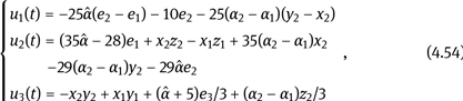
To study synchronization between two unified chaotic systems with different initial values and different certain parameters, the parameters of the drive system and response system are set to be α1 and α2, respectively, and the drive system equation is

The response system equation is

To realize the synchronization, the control functions u1(t), u2(t), and u3(t) are added to the right-hand side of each equation, and the response system becomes

The error system is obtained by subtracting eq. (4.52) from eq. (4.50)

where synchronization error e1 = x2 – x1, e2 = y2 – y1, and e3 = z2 – z1. Obviously, the problem of synchronization between two chaotic systems with different parameter is transformed into the stability problem of error system (4.53) at the origin e1 = 0, e2 = 0, and e3 = 0. If the appropriate control variables u = [u1(t), u2(t), u3(t)]T is chosen to make error system (4.53) stable, then response system (4.51) can be synchronized with drive system (4.50).
Theorem 4.6: For drive system (4.50) and response system (4.51), if we choose the control function
where the parameter ![]() is an estimate of the parameter α1, and the adaptive law of the estimate parameter is
is an estimate of the parameter α1, and the adaptive law of the estimate parameter is ![]() If the control parameter satisfy λ ≥ 0, then the equilibrium point e = 0 and α1 = α̂ exist in the error system, and the asymptotic synchronization is realized between the response system and drive system. That is,
If the control parameter satisfy λ ≥ 0, then the equilibrium point e = 0 and α1 = α̂ exist in the error system, and the asymptotic synchronization is realized between the response system and drive system. That is, ![]() for any initial values.
for any initial values.
Proof. Substitute control function (4.54) into error system (4.53), then we have

So error dynamics system (4.55) has no relationship with the response system parameter α2. As long as the error system is stable, it can realize the synchronization of two chaotic systems with different parameters. According to the Lyapunov stable theory, the Lyapunov function is constructed as
where e = [e1, e2, e3]T, ![]() = α1 – α̂. If the adaptive law of the estimate parameter is
= α1 – α̂. If the adaptive law of the estimate parameter is
then the derivative of eq. (4.56) is
Substituting eq. (4.55) and eq. (4.57) into eq. (4.58), we have
According to the Lyapunov stable theory, when λ ≥ 0, Ė≤ 0, and equilibrium point e = 0, α1 = α̂. The error system is asymptotically stable, so the two systems are synchronized. ∎
We use Matlab/Simulink for numerical simulation. Set α1 = 0.8, α2 = 0.3, and initial values x1(0) = 10, y1(0) = 10, z1(0) = 10, x2(0) = –5, y2(0) = –5, z2(0) = –5 and α̂(0) = 0.5, and do numerical simulation for control parameter λ = –0.1, λ = 1, λ = 2, and λ = 5. The synchronization error curves between the two chaotic systems with different control parameters are shown in Figure 4.18.

Figure 4.18: Synchronization error curve with different control parameters: (a) + = –0.1; (b) + = 1; (c) + = 2; and (d) + = 5.
The following conclusions are obtained by theoretical analysis and simulations. (1) The performance of the synchronization system can be improved by increasing the control parameter, and the monotonous synchronization of two chaotic systems is realized as shown in Figure 4.18(b)–(d). (2) The selection of the initial value of the adaptive parameters has no effect on the results. For example, the synchronization error curve with α1 = 0.3, α̂(0) = 2, and λ = 5 is the same with that with α1 = 0.8, α̂(0) = 0.5, and λ = 5 as shown in Figure 4.18(d). (3) There is parameter λ that does not meet the synchronization conditions, but it can make the synchronization of two systems [99], as shown in Figure 4.18(a), while the performance is poor at this time.
4.5.2Adaptive Synchronization Control with Uncertain Parameters
Taking the unified chaotic system as an example, the synchronization of two chaotic systems with unknown parameters is discussed.
When the two system parameters are unknown, the drive and response systems based on unified chaotic system are


where v = [v1, v2, v3]T is the control vector and α is the unknown parameter. Set the error variables as e1 = x2–x1, e2 = y2–y1, and e3 = z2–z1, then the error system of systems (4.60) and (4.61) is

To make the error system stable and realize the synchronization between the two systems, the following theorem is proposed for the control function and the estimated parameters.
Theorem 4.7: For drive system (4.60) and response system (4.61), if the control function is defined as

the parameter ![]() is the estimate of the parameter α. If the adaptive law of the estimate parameter is
is the estimate of the parameter α. If the adaptive law of the estimate parameter is ![]() then there exist the equilibrium points e = 0 and α = α̂ in the error system, and the asymptotic synchronization is realized between the response system and drive system. That is,
then there exist the equilibrium points e = 0 and α = α̂ in the error system, and the asymptotic synchronization is realized between the response system and drive system. That is, ![]() for any initial values.
for any initial values.
Proof. Substituting control function (4.63) into error system (4.62), we have

As long as the error system is stable, the synchronization of two chaotic systems with uncertain parameters is realized. According to the Lyapunov stable theory, the Lyapunov function V is constructed as
where α = α – α̂, and α̂ is the estimate of uncertain α. If we choose the adaptive law of the estimate parameter ![]() then the derivative of eq. (4.65) is
then the derivative of eq. (4.65) is
Because V is positive, and α ≥ 0, V̇ is negative. According to the Lyapunov stable theory, there are equilibrium points e = 0 and α = α̂, that is,
The response system and the drive system are synchronized. ∎
We use Matlab/Simulink for numerical simulation. When α ∈ [0, 1], both drive system (4.60) and response system (4.61) are chaotic. Let the initial values x1(0) = 10, y1(0) = 10, z1(0) = 10, x2(0) = –5, y2(0) = –5, z2(0) = –5, and α ∈ [0, 1], α̂(0) = 0.5. The synchronization error curve of two chaotic systems with unknown parameters is shown in Figure 4.19. The phase diagram of variables x1 and x2 is displayed in Figure 4.20.
The following conclusions are obtained by theoretical analysis and simulations. (1) The performance of the synchronization is stable as shown in Figure 4.19. When steady-state error is Δφ = 10–4, the setup time of synchronization system is short (t < 2 s), and the monotonous synchronization of two systems is achieved. (2) The selection of the initial value of the adaptive parameters has no effect on the results. For example, the synchronization error curve with α̂(0) = 2 is the same with that with α̂(0) = 0.5. (3) By the Lyapunov stability theory, the synchronization condition is only a sufficient condition.

Figure 4.19: Error curve of chaotic synchronization system.

4.6Intermittent Feedback Synchronization Control
Among the synchronization control methods, the intermittent feedback control method is used to obtain the desired synchronization at low cost, and it is simple and easy to realize. In this section, the intermittent feedback synchronization between the unified chaotic system and its deformation system is investigated.
4.6.1Intermittent Synchronization Control between Different Systems
Here, we discuss the problem of intermittent synchronization between two different chaotic systems with topological similarity. For the unified chaotic system

When the parameter α ∈ [0, 1], the system is chaotic.
The deformation system of the unified chaotic system is [100]

Correspondingly, when α = 0.8, systems (4.68) and (4.69) are Lü system and deformation Lü system, respectively. The phase portraits with the initial value [–1, 1, 0] are shown in Figure 4.21. Obviously, the phase track curves of Lü system and deformation Lü system are similar, but the evolution of the deformation system in the phase space is more divergent and the system is more complex.

Figure 4.21: Strange attractors with α = 0.8: (a) Lü system and (b) deformation Lü system.
To realize the synchronization between chaotic system (4.68) and deformation system (4.69), the synchronization control signal ui(t) is added to eq. (4.69), and then eq. (4.69) becomes

Set ei = xi–yi, then the error system equation is

Set the control variables to

where p(t) is a pulse signal with period T and the ratio D of pulse length and pulse period, and it is defined by
It can be seen that eq. (4.72) is a composite controller composed of nonlinear continuous feedback and linear intermittent feedback. So, eq. (4.71) becomes

If it is asymptotically stable at the origin, the synchronization between systems (4.68) and (4.70) is achieved.
Theorem 4.8: For systems (4.68) and (4.69), if it is controlled by eq. (4.72), and the feedback parameter satisfies k > 27–6α, and D ≥ 0.4, then the asymptotically stable synchronization will be realized between systems (4.70) and (4.68).
Proof. Decompose the error system eq. (4.74), and when iT < t < iT + TD, we have

where A1 is the Jacobian matrix of the error system when the system has a control pulse

When iT + TD < t < (i + 1)T, we have

where A2 is the Jacobian matrix of the error system when the system has no control pulse

and ![]() is the nonlinear term of the error system. For all t, when ‖e‖ →0,
is the nonlinear term of the error system. For all t, when ‖e‖ →0, ![]() , so the evolution of errors depends on A1 and A2. During iT < t < iT + TD, the error is controlled by A1. For α ∈ [0, 1], according to the stability criterion of continuous system, if k satisfies k > 27–6α, then the eigenvalues of the matrix A1 have negative real part. The zero point of the error system is asymptotically stable at this time. During iT + TD < t < (i + 1)T, the controlled systems lose some additional feedback, and the error is controlled by A2. Because A2 does not satisfy the stability condition, the trajectory of the two systems will diverge, and the synchronization of the two systems will be lost. As long as the error is still small enough, and the exert control pulse is applied again, it can ensure that the error will not deviate too far, so that the synchronization of the two systems will be achieved gradually. After the continuous system is discretized, the error equation is written as
, so the evolution of errors depends on A1 and A2. During iT < t < iT + TD, the error is controlled by A1. For α ∈ [0, 1], according to the stability criterion of continuous system, if k satisfies k > 27–6α, then the eigenvalues of the matrix A1 have negative real part. The zero point of the error system is asymptotically stable at this time. During iT + TD < t < (i + 1)T, the controlled systems lose some additional feedback, and the error is controlled by A2. Because A2 does not satisfy the stability condition, the trajectory of the two systems will diverge, and the synchronization of the two systems will be lost. As long as the error is still small enough, and the exert control pulse is applied again, it can ensure that the error will not deviate too far, so that the synchronization of the two systems will be achieved gradually. After the continuous system is discretized, the error equation is written as

where e(i) is the error vector of the ith pulse period. DT = m1h, (1 – D)T = m2h, where h is the integral step size, and m1, m2 are the integral iteration numbers for a pulse and no pulse, respectively. Obviously, in the process of synchronization, the system will generate oscillation due to (A2)m2, and the stable synchronization process will depend on |(A1)m1 (A2)m2 |. If |(A1)m1 (A2)m2| = |J| < 1, then the system will become stable [101]. The exact range of D can be obtained by numerical experiments. Simulations show that when D ≥ 0.4, the exact synchronization can be achieved within 10 s. ∎
4.6.2Synchronization Simulation and Performance Analysis
The synchronization control and performance improvement for the unified chaotic system and its deformation system are studied based on Matlab simulation. Here, we observe the changes of the time performance of the synchronization from the aspects of the initial value, the feedback coefficient k, the proportion factor D, the step size h, and the system parameter α.
4.6.2.1Effect of Initial Value on Synchronization Performance
Set α=0.8, k =40, T =0.1 s, D=0.6, h = 0.001, and the initial values are (1) X(0) = [20, 0, 0], Y(0) = [–2, 1, 0]; (2) X(0) = [10, 0, 0], Y(0) = [–2, 1, 0]; and (3) X(0) = [5, 0, 0], Y(0) = [–2, 1, 0]. The synchronization error curve is shown in Figure 4.22. So, the synchronization between the two systems is achieved within 1.5 s. The oscillation phenomenon occurs in the process of establishing the synchronization, which is related to the characteristic value of A2. Because at the beginning of iT + TD < t < (i + 1)T, the error has not reached the steady state. In addition, the oscillation for initial value (3) is minimum, while the oscillation for initial value (1) is maximum. It can be seen that the initial value of the two systems is more; the larger the oscillation, the more the time required to establish accurate synchronization. But in general, it can achieve satisfactory results even when the initial value is large.
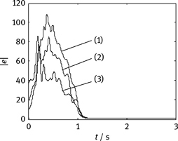
Figure 4.22: Synchronization error curves for different initial values.

4.6.2.2Effect of different k, D, and h on synchronization performance
Set α = 0.8, T = 0.1 s, D = 0.8, and h = 0.0001, and the initial values are X(0) = [5, 0, 0] and Y(0) = [–2, 1, 0]. When the k values are 42, 32, and 27, the synchronization error curves are shown in Figure 4.23. It shows that the smooth degree of the curve is different with different k. For example, the error converges quickly for k = 27, and the error converges the fastest for k = 42. So the establishment time of the synchronization decreases with the increase of k, which is consistent with the theoretical analysis. In the practical application, considering the cost and the difficulty of the realization, the value of k should not be too large.
To achieve synchronization, the regulation of D is also important. Numerical experiments show that, similar to k, the synchronization setup time decreases with the increase of D. Further experiments prove that the smaller the size of the h is, the smaller the oscillation time is, and the faster the error curve converges.

4.6.2.3Effects of different parameter α on synchronization performance
Let k = 45, T = 0.1 s, D = 0.6, andh = 0.0001, and the initial values are X(0) = [15, 0, 0], Y(0) = [–15, –15, –15]. The relationship of the synchronization setup time tb with the parameter α is shown in Figure 4.24. It shows when α ∈ [0, 1], the synchronization between the unified chaotic system and its deformation system is achieved within about 4 s, and the synchronization setup time decreases with increase of α.
4.7Synchronization Control Based on State Observer Method
Because this synchronization method does not need to calculate the conditional Lyapunov exponent, it is widely concerned.
4.7.1Design Principle of State Observer
Consider a class of nonlinear feedback chaotic systems

where x ∈ Rn, u ∈ Rk, and w ∈ Rm are the state variables, nonlinear feedback input, and random noise of the system, respectively. y is the output in the sender. A, B, C, and E are known constant matrices.
In the receiver, when the nonlinear feedback input u is measurable, then the state observer of the system can be expressed as [102]
where z ∈ Rn and ![]() ∈ Rn. F, G, H, and J are unknown constant matrices.
∈ Rn. F, G, H, and J are unknown constant matrices.
Suppose In is a unit matrix with n order, the error of the state observer is defined as e = x̂ – x = z – (In + JCT)x. Let M = In + JCT, then the dynamic equation of the error system is
When error system (4.82) satisfies

then the error system becomes ė = Fe. Obviously, if all eigenvalues of the matrix F are less than zero, then ![]() converges to x exponentially.
converges to x exponentially.
Substitute M = In + JCT into the third term of HCT – MA + FM = 0, then we have
Let
and substitute eq. (4.84) into eq. (4.85), then we obtain
At this point, the state observer equation is changed to
So, the design problem of the state observer with random disturbance is turned into the problem of how to find the appropriate J, which satisfies (In + JCT)E = 0, and how to choose the appropriate N, which satisfies the eigenvalues of F are less than zero. As F = MA–NCT, the condition that the eigenvalues of F are less than zero must be satisfied by choosing appropriate N. That is to say, in this case, we can always find a suitable N, so that when t →∞, x̂ converges to x exponentially.
From eq. (4.83), we obtain JCTE = –E, and according to matrix knowledge, we have
where (CTE)+ is the generalized inverse matrix of (CTE). V is the matrix with appropriate dimensions. For the convenience of application, we often let V = 0. Then we have J = –E(CTE)+. At the same time, we can obtain M = Ip + JCT.
4.7.2Design of State Observer for Unified Chaotic System
By applying the state observer method to the unified chaotic system, the sender matrix is described as

The receiver equation is

where

Here, n1, n2, and n3 are the three values of the one-dimensional vector N, which can ensure that the eigenvalues of matrix F are less than zero, and these lead the synchronization error for ė = Fe to zero finally. For simple calculation, we set n1 = 25α+10, n2 > 0, n3 = 0. When t →∞, x̂ converges to x exponentially.
4.7.3Simulation and Discussion
Based on Matlab simulation platform, the synchronization of the unified chaotic system is investigated in this section. We set the initial values x1(0) = 15, x2(0) = 15, x3(0) = 15, x̂1(0) = 10–10, x̂2(0) = –10, x̂3(0) = 10–10; n1 = 25α + 10, n3 = 0, and let the synchronization error

Next, we study the synchronization performance of the synchronization system.
4.7.3.1Synchronization Performance with Different Parameter α
When n2 = 3 and w(t) = 100 sin(3t), we obtain the synchronization error curves for α = 0.5, α = 0.8, α = 0.9, respectively, as shown in Figure 4.25. It can be seen, although the difference between the two initial values is very far, that the system can achieve synchronization within t = 2 s for different system parameters. It shows that the system has strong robustness to parameter variation.
4.7.3.2Effect of Noise Interference on the Performance of System Synchronization
When n2 = 3 and α = 0.8, we obtain the synchronization error curves for w(t) = 5 sin(3t), w(t) = 100 sin(3t), and white noise, respectively, as shown in Figure 4.26. It can be seen that the type and size of the noise have little effect on the synchronization error signal. The system can achieve the precise synchronization within t = 2 s. It shows the method has strong antinoise performance.
4.7.3.3Effect of Initial Values on the Performance of System Synchronization
When n2 = 3, α = 0.8, and w(t) = 100 sin(3t), we obtain the synchronization error curves for following initial values as shown in Figure 4.27.
(1) X(0) = [15, 15, 15] X̂(0) = [10–10, –10, 10–10],
(2) X(0) = [50, 50, 50] X̂(0) = [10–10, –10, 10–10],
(3) X(0) = [15, 15, 15] X̂(0) = [10, 5, 10].

Figure 4.25: Synchronization error curves for different α.


From Figure 4.27, the setup time for the system synchronization is the longest for (2), and the setup time for the system synchronization is the shortest for (3). Because the synchronization error signal e(t) decays exponentially, the time required to determine the exact synchronization is related to the initial conditions of the transmission end and the receiving end. It is obvious that the difference of the two initial values for (2) between the sender and the receiver is the biggest, so it is the longest time to achieve the exact synchronization.
4.7.3.4Effect of Different n2 on the Performance of Synchronization System
When w(t) = 100 sin(3t), α = 0.8, we obtain the synchronization error curves for n2 = 1, n2 = 5, and n2 = 50, respectively, as shown in Figure 4.28. Obviously, when n2 > 0, then the larger the n2 is, the shorter the synchronization time of the system is. But when n2 exceeds a certain value, then the value of n2 is increased, and the time needed for synchronization is not significantly reduced.

4.8Chaos Synchronization Based on Chaos Observer
4.8.1Design Principle of Chaos Observer
For the following chaotic system
where x ∈ Rn, F: Rn →Rn; s is the scalar output of the system. Set k(x) is a scalar differentiable function, and V(x) is vector field, where V: Rn →Rn. Lee derivative of the vector field V(x) along the scalar differentiable function k(x) is defined as Lvk, then Lvk = <V(x) ● grad k(x)>, where < ● > is the Euclidean inner product. The ith Lee derivative of the vector field V(x) along the scalar differentiable function k(x) is defined as ![]()
Lemma 4.1 [103]: If ![]() is diffeomorphism, then all the state variables of system (4.92) are observable by using scalar output s and it is the ith (i ≤ n – 1) Lee derivative, and x = ϕ–1[s(t), s(1)(t), . . . , s(n–1)(t)]T.
is diffeomorphism, then all the state variables of system (4.92) are observable by using scalar output s and it is the ith (i ≤ n – 1) Lee derivative, and x = ϕ–1[s(t), s(1)(t), . . . , s(n–1)(t)]T.
If a state variable xi is selected as the output of system (4.92), then the remaining state variables of system (4.92) can be expressed as ![]() where j ≠ i. So system (4.92) is written as
where j ≠ i. So system (4.92) is written as
where A is a constant matrix, and ![]() is a matrix with n×1 order, which includes all the nonlinear terms of system (4.92).
is a matrix with n×1 order, which includes all the nonlinear terms of system (4.92).
Lemma 4.2 [104]: Set the output of system (4.92) as
where B = diag[b1, b2, . . . , bn]. If we select an appropriate diagonal matrix B so that the eigenvalues of the matrix A–B have a negative real part, then system ẏ = F(y) + s(x) – s(y) is the chaos observer of chaotic system (4.92), where ![]()
![]()
4.8.2Chaos Observer of the Unified Chaotic System
The state observer synchronization scheme is applied to the unified chaotic system, and we have

Here, the drive system is driven by

where

The state observer system in the receiver can be expressed as
where ![]() is similar with s(x).
is similar with s(x).
By eq. (4.95), when the appropriate B is taken, the characteristic value of the A–B is negative, and then the accurate synchronization between the chaotic system in the sender and the state observer in the receiver can be achieved.
4.8.3Synchronization Simulation and Performance Analysis
The synchronization simulation of the unified chaotic system is carried out on Matlab, and we set the system’s initial conditions x1(0) = 1, x2(0) = 1, x3(0) = 1, x̂1(0) = 15, x̂2(0) = 15, x̂3(0) = 15,

where b22 > 19α – 1, and let ei = (x̂i – xi).
Next, we will study the synchronization performance of the synchronization system.
4.8.3.1Effect of Different Parameter α on the Performance of System Synchronization
For simulation, we set α = 0.5, α = 0.8, and α = 0.9 (it means the system is the generalized Lorenz system, the generalized Lü system, and the generalized Chen system respectively). The synchronization error curves are obtained as shown in Figure 4.29. Obviously, for different parameter α, the unified chaotic system and the state observer will achieve accurate synchronization, but the synchronization performance is not exactly the same. This is mainly due to the use of a single parameter transmission, and the function between x2 and x̂2 is complex. So this calculation will have a greater impact on the synchronization performance between x2 and x̂2 with different α values. Overall, the synchronization performance is good for different α values.
4.8.3.2Effect of Initial Values on the Performance of System Synchronization
Setting b22 = 29 and α = 0.8, the changes of the synchronous error signals with the following three different initial conditions are analyzed, respectively. The synchronization error curves of the system are shown in Figure 4.30:
Initial condition (1): X(0) = [ 15, 15, 15 ] X̂(0) = [ 10–10, –10, 10–10 ].
Initial condition (2): X(0) = [ 50, 50, 50 ] X̂(0) = [ 10–10, –10, 10–10 ].
Initial condition (3): X(0) = [ 15, 15, 15 ] X̂(0) = [ 10, 5, 10 ].
From Figure 4.30, when the initial values between the unified chaotic system and the state observer are further away from each other, the oscillation is more obvious, and the time required for synchronization is longer, which is consistent with the conclusion obtained by the previous state observer method. However, even if the initial value of the two is far, the system can still achieve accurate synchronization.

Figure 4.29: Synchronization error curves for different α: (a) α = 0.5; (b) α = 0.8; and (c) α = 0.9.
4.8.3.3Effect of Different b22 on the Performance of Synchronization System
When α = 0.8, system initial values x1(0) = 1, x2(0) = 1, x3(0) = 1, x̂1(0) = 15, x̂2(0) = 15, x̂3(0) = 15, and b22 =24, b22 =30, b22 = 50, respectively, we obtained the synchronization error curves as shown in Figure 4.31. It shows that with the increase of b22, the oscillation amplitude is smaller and smaller before the system reaches synchronization, and the time required to achieve synchronization is also less and less, but the corresponding hardware requirements will be higher. So in practical applications, the appropriate increase of b22 is good for improving the performance of system synchronization. In short, the system can achieve accurate synchronization in a certain time, as long as the condition b22 > 29α – 1 is satisfied.
The chaos synchronization scheme, which is based on the state space reconstruction technique, is relatively simple in design and calculation. In the process of synchronization, the single parameter is transmitted, and the other parameters are derived at the receiving end. In this way, the channel utilization rate is greatly improved. As far as the synchronization performance, the proposed scheme has the characteristics of short synchronization time and good synchronization performance. However, the synchronous curve is not monotonous, and the oscillation is obvious; so, in practical application, to make the system synchronization performance optimization, the selection of the system parameters is the key.

Figure 4.30: Synchronization error curves for different initial conditions: (a) initial value (1); (b) initial value (2); and (c) initial value (3).
4.9Projective Synchronization
In 1999, Mainieri and Rehacek [28] observed a new synchronization phenomenon in the study of partially linear chaotic systems namely projective synchronization. For some partially linear chaotic systems, when the proper controller is selected, the output phase of the drive–response system state can be locked, and the amplitude of each corresponding state is also evolving according to a certain ratio. The new synchronization phenomenon has been greatly concerned by researchers, and a variety of projection synchronization schemes are proposed. Recently, a function projection synchronization method was proposed [29]. When compared with the general projective synchronization, the function projection synchronization means that the drive system and the response system can be synchronized according to a certain function, which is significant for the chaotic secure communication. In engineering practice, the parameters of the system may be unknown. To realize the parameter identification of chaotic systems with unknown parameters, the adaptive synchronization method is applied to the synchronization of chaotic systems with unknown parameters [29–30]. So it is important to study the projective synchronization control of chaotic systems, especially to study the synchronization of chaotic systems by combining adaptive control and function projective synchronization.

Figure 4.31: Synchronization error curves for different b22: (a) b22 = 24; (b) b22 = 30; and (c) b22 = 50.
4.9.1Principle and Simulation of Proportional Projection Synchronization
Consider the following continuous chaotic system:
where the state variable X = (x1, x2, . . . , xn)T ∈ Rn, and the continuous vector function F: Rn → Rn. The function F (X) is decomposed into
where ÃX is the linear part of F (X), and ![]() (X) is the nonlinear part of F (X). Then, ÃX is decomposed into
(X) is the nonlinear part of F (X). Then, ÃX is decomposed into
where A is a full rank constant matrix, and the real part of the eigenvalue is negative. Let
then eq. (4.96) can be rewritten as
Now, we take system (4.100) as the drive system and employ the projective synchronization control method. Then the response system is
where Y ∈ Rn is the n-dimensional state vector of the response system, and α is the proportional coefficient. If the synchronization error between drive system (4.100) and response system (4.101) is E = X – αY, then the synchronous error equation is
The real part of all eigenvalues of matrix A is negative, so synchronous error system (4.102) is asymptotically stable at the origin according to the stability criterion of linear system. That is, ![]() So the synchronization is achieved between response system (4.101) and drive system (4.100).
So the synchronization is achieved between response system (4.101) and drive system (4.100).
Applying the projective synchronization method to the simplified Lorenz chaotic system, the drive system becomes

and the response system becomes

where α is the proportional coefficient (α ≠ 0), and b is the synchronization control parameter. For the synchronization system comprising systems (4.103) and (4.104), the following synchronization theorem is proposed.
Theorem 4.9: For the projection synchronization system composed by drive system (4.103) and response system (4.104), if the synchronization control parameter b < min[10, 4c–24], then the synchronization error system is asymptotically stable at the origin point. That is, response system (4.104) will be synchronized with drive system (4.103) according to the proportional α.
Proof. According to the principle of projective synchronization, for the projection synchronization system comprising drive system (4.103) and response system (4.104), the full rank matrix A and H(X) are, respectively,

If λ is the eigenvalue of the matrix A, then we have

Obviously, one of the eigenvalues λ1 = –8/3 and the other two characteristic roots satisfy the equation
According to the Routh–Hurwitz criterion, if the synchronization control parameter satisfies b < min[10, 4c–24], then the real part of the root of eq. (4.106) is negative. The parameter of the system c ∈ [–1.59, 7.75], so we get b < –17.64. That is, when the control parameter of the synchronization system is b < –17.64, the real part of all eigenvalues of the matrix A of the synchronization error system is negative, and the synchronization error is ![]() It means response system (4.104) will be synchronized with drive system (4.103) according to the ratio α. ∎
It means response system (4.104) will be synchronized with drive system (4.103) according to the ratio α. ∎
On Simulink dynamic simulation platform, we set c = 5. According to Theorem 4.9, when b < –4, the synchronization will be achieved. Here we set b = –5 and α = –2, and system initial values x1(0) = 4.4356, x2(0) = 6.1771, x3(0) = 7.2330; y1(0) = 2.0883, y2(0) = 0.4535, y3(0) = –5.8578. The error convergence curve, the evolution of the attractor, and variable of the chaotic synchronization system are shown in Figure 4.32, where the synchronization error is defined by ![]() Figure 4.32(a) shows that the two chaotic systems with different initial values can achieve the projective synchronization at about 7.0 s, and the dynamic characteristics of the synchronization is good. Figure 4.32(b) shows that the attractor of the response system and drive system is inverse, and the size ratio is 2:1. According to Figure 4.32(c), we can see that the response system variable y3 is synchronized with the drive system variable x3 according to the projection ratio.
Figure 4.32(a) shows that the two chaotic systems with different initial values can achieve the projective synchronization at about 7.0 s, and the dynamic characteristics of the synchronization is good. Figure 4.32(b) shows that the attractor of the response system and drive system is inverse, and the size ratio is 2:1. According to Figure 4.32(c), we can see that the response system variable y3 is synchronized with the drive system variable x3 according to the projection ratio.

Figure 4.32: Projective synchronization between systems (4.103) and (4.104): (a) synchronization error curve; (b) attractors; and (c) waves of variables x3 and y3.
Now, we analyze the effects of different b values on the synchronization performance of the synchronization system. Set c = 5, α = –2, and the initial values are same with that of Figure 4.32. Simulations are carried out for b = –5, b = –6, b = –15, respectively. The synchronization error curves are plotted in Figure 4.33. When b < –4, the smaller the b, the shorter the time required to achieve synchronization, but when b exceeds a certain value, then b reduces further, and the time required for synchronization cannot be significantly reduced. By formula (4.106), the b value is smaller, and the real part of the characteristic value of the synchronization error system is more negative. The pole is farther from the virtual axis; the faster the convergence of the synchronization system, the shorter the synchronization setup time.

Figure 4.33: Synchronization error curves for different control parameter b: (a) b = –5; (b) b = –6; and (c) b = –15.
4.9.2Principle and Simulation of Function Projective Synchronization
Consider the following continuous-time chaotic system as the drive system
where X = (x1, x2, . . . , xn)T ∈ Rn is the state variable. AX is the linear part, and F (X) is the nonlinear part. Copy eq. (4.107), and add the controller U: R2n → Rn into the system, then the response system is
where Y = (y1, y2, . . . , yn)T ∈ Rn is the state vector. Set as the function matrix, and the error function of the synchronization system is E = X – Φ(t)Y. By designing the controller U (X, Y), we can get ![]() and then the generalized function projective synchronization is achieved between systems (4.107) and system (4.108).
and then the generalized function projective synchronization is achieved between systems (4.107) and system (4.108).
Applying the generalized function projective synchronization method to the simplified Lorenz system, the drive system and response system are, respectively,


where c is the system parameter, and U = [u1, u2, u3]T is the nonlinear controller. We have the following synchronization theorem for the synchronization system comprising systems (4.109) and (4.110).
Theorem 4.10: For systems (4.109) and (4.110), the control law is U(X, Y) = Φ–1(t)[–(t)Y + F (X) – Φ(t)G(Y) + (A – B)X + DE], where Φ(t) is the projective function, and D = diag[d1, d2, d3] is the control parameter matrix. When the controller parameter satisfies d1 + d2 > c–10, d1d2–d1c + 10d2 > 240–30c, and d3 > –8/3, systems (4.109) and (4.110) can realize the function projective synchronization, that is, ![]() for any initial value.
for any initial value.
Proof. For the projection synchronization system comprising drive system (4.109) and response system (4.110), the error function of the synchronization system is
where Φ(t) is the diagonal function matrix. Then the error system equation is
Substituting eqs (4.109) and
If the controller is U (X, Y) = Φ–1(t)[–Φ̇ (t)Y + F (X) – Φ(t)G(Y) + (A–B)X + DE], then we obtain
Construct Lyapunov function V(t) as
Then its differential is
Substituting eq. (4.114) into the above formula, we have
Set the control matrix D = diag[d1, d2, d3], when d1+d2 > c–10, d1d2–d1c+10d2 > 240– 30c, and d3 > –8/3, D–B is positive, and then ![]() ≤ 0 if and only if E = 0 for equality. By the Lyapunov stability theorem, the error system of the drive–response system is asymptotically stable at the origin. That is,
≤ 0 if and only if E = 0 for equality. By the Lyapunov stability theorem, the error system of the drive–response system is asymptotically stable at the origin. That is, ![]() The function projection synchronization is implemented. ∎
The function projection synchronization is implemented. ∎
On Simulink dynamic simulation platform, we set c = 5. According to Theorem 4.10, when the control parameters are d1 =40, d2 =20, d3 = – 2, the synchronization will be achieved. Set the projective function Φ(t) = – 3 + 2 sin t, and the initial values x1(0) = 4.4356, x2(0) = 6.1771, x3(0) = 7.2330; y1(0) = – 1.8028, y2(0) = – 2.3247, y3(0) = – 2.2974. The synchronization error convergence curve, the evolution of the attractor, and variable of the chaotic synchronization system are shown in Figure 4.34. Figure 4.34(a) shows that the two chaotic systems with different initial values can achieve the projective synchronization within 4.8 s, and the dynamic characteristics of the synchronization are good. Figure 4.34(b) shows that the attractor of the response system and drive system is inverse, and the size ratio satisfies the projective function. According to Figure 4.34(c), we can see that the response system variable y3 is synchronized with the drive system variable x3 according to the projection function.

Figure 4.34: Projective synchronization between systems (4.109) and (4.110): (a) Synchronization error curve; (b) attractors; and (c) waves of variables x3 and y3.
Now, we analyze the effects of different control parameter d1, d2, d3 on the synchronization performance of the synchronization system. Set the system parameter c = 5, the projective function Φ(t) = –3 + 2 sint, and the initial values x1(0) = 4.4356, x2(0) = 6.1771, x3(0) = 7.2330; y1(0) = –1.8028, y2(0) = –2.3247, y3(0) = –2.2974.
- When d2 = 20, d3 = –2, then d1 > –7.3 according to Theorem 4.10. Synchronization simulations are carried out for d1 = –7, d1 = –6.7, d1 = –5, respectively. The synchronization error curves are plotted in Figure 4.35(a). Obviously, when d1 > –7.3, the bigger the d1, the shorter the time required to achieve synchronization, but when the d1 exceeds a certain value, and then continue to increase d1, the time required for synchronization cannot be significantly reduced.
- When d1 = 40 and d3 = –2, then d2 > 5.8 according to Theorem 4.10. Synchronization simulations are carried out for d2 = 6.15, d2 = 6.5, d2 = 7, respectively. The synchronization error curves are plotted in Figure 4.35(b). Obviously, when d2 > 5.8, the bigger the d2, the shorter the time required to achieve synchronization, but when the d2 exceeds a certain value, and continue to increase d2, the time

Figure 4.35: Synchronization error curves for different control parameter d. (a) Curve 1: d1 = –7; curve 2: d1 = –6.7; curve 3: d1 = –5. (b) Curve 1: d2 = 6.15; curve 2: d2 = 6.5; curve 3: d2 = 7. (c) Curve 1: d3 = –2.3; curve 2: d3 = –2; curve 3: d3 = 0. required for synchronization cannot be significantly reduced.
3.When d1 = 40 and d2 = 20, then d3 > –8/3 according to Theorem 4.10. Synchronization simulations are carried out for d3 = –2.3, d3 = –2, d3 = 0, respectively. The synchronization error curves are plotted in Figure 4.35(c). Obviously, when d3 > –8/3, the bigger the d3, the shorter the time required to achieve synchronization, but when the d2 exceeds a certain value, if we continue to increase d3, the time required for synchronization cannot be significantly reduced.
4.9.3Principle and Simulation of the Adaptive Function Projective Synchronization
Consider the following drive system and response system:
where θ and δ are unknown parameter vectors in the drive system and the response system, respectively. f (X) and g(Y) are vector functions of state variables X and Y. F (X) and G(Y) are function matrices. U (X, Y) is the control law.
Supposing the projective function is Φ(t), and the error function of the synchronization system is E = X –Φ(t)Y, then the synchronization error system equation is
Due to eqs (4.118) and (4.119), we have
where M(X, Y) = f(X)–Φ(t)g(Y)+(A–B)X. Obviously, the adaptive function projective synchronization problem of drive system (4.118) and response system (4.119) is transformed into the stability problem of eq. (4.121). By designing the controller U(X, Y) and the adaptive law, to make ![]() the adaptive function projective synchronization between systems (4.118) and (4.119) can be realized and the unknown parameters can be identified.
the adaptive function projective synchronization between systems (4.118) and (4.119) can be realized and the unknown parameters can be identified.
Theorem 4.11: For the chaotic synchronization system with unknown parameter, which is composed of drive system (4.118) and response system (4.119), if the control function of the system is U(X, Y) = Φ–1(t)[M(X, Y) + F(X)θ̂ – Φ̇ (t)Y – Φ(t)G(Y)δ̂̇ + DE], where M(X, Y) = f(X) – Φ(t)g(Y) + (A – B)X, and D = diag[d1, d2, d3]. If the appropriate control parameters and the adaptive law of the system parameters are selected as = FT(X)E + Bθ, ˙δ̂ = –Φ(t)GT(Y)E + Bδ, where θ̂ = θ – θ̂, δ̄ = δ – δ̂̇. The adaptive function projective synchronization is realized between systems (4.118) and (4.119), and the unknown parameters are identified correctly. That is, for any initial values, we have ![]()
![]() = θ, and
= θ, and ![]() = δ.
= δ.
Proof. Choose U(X, Y) =Φ–1(t)[M(X, Y) + F(X)θ̂ – Φ̇ (t)Y –Φ(t)G(Y)δ̂ + DE] as the controller, then the error system eq. (4.120) becomes
Constructing Lyapunov function
where θ̄ = θ – θ̂ , δ̄ = δ – δ̂, then its differential is
Set the adaptive law as ![]() = FT(X)E + θ̄ and
= FT(X)E + θ̄ and ![]() = – Φ(t)GT(Y)E + δ̄, and substitute eq. (4.121) into eq. (4.124), then we have
= – Φ(t)GT(Y)E + δ̄, and substitute eq. (4.121) into eq. (4.124), then we have
Obviously, if we choose control parameters d1, d2, and d3, to make (D–B) positive definite, then we have V̇ ≤ 0. If and only if E = 0, θ̄= 0, δ̄ = 0 for equality. By the Lyapunov stability theorem, the error system of the drive–response system is asymptotically stable at the origin. That is, ![]() and the adaptive function projection synchronization is implemented. At the same time, when t→∞, we have θ̂→θ and δ̂→δ. That is, the unknown parameters are identified correctly. ∎
and the adaptive function projection synchronization is implemented. At the same time, when t→∞, we have θ̂→θ and δ̂→δ. That is, the unknown parameters are identified correctly. ∎
Remark 1: If A = B, f (⋅) = g(⋅), and F(⋅) =G(⋅), then the two chaotic systems are homogeneous systems, and vice versa they are heterogeneous systems. Therefore, the adaptive function projective synchronization theorem can be applied to both homogeneous and heterogeneous systems with unknown parameters.
Remark 2: If the parameters of the drive system or response system are known, using the above control method, the parameter adaptation law is removed, and the corresponding generalized function projective synchronization can be realized.
4.9.3.1Adaptive Function Projective Synchronization and Simulation for Driving System with Unknown Parameters
Applying the adaptive function projective method to the simplified Lorenz system, the drive system and response system are, respectively,


where c is the system parameter. C = [θ1, θ2, θ3]T is the unknown parameter of the drive system. U = [u1, u2, u3]T is the nonlinear controller. If we set the projective function as Φ(t) = –3 + 2sin(t), according to Theorem 4.11, the control law and the parameter adaptive law of the synchronization system consisting of systems (4.126) and (4.127) are


There is a following inference for the synchronization system consisting of systems (4.126) and (4.127).
Inference 4.2 For the adaptive function projective synchronization system comprising drive system (4.126) and response system (4.127), when the controller parameters satisfy d1 + d2 > c–10, d1d2–d1c + 10d2 > 240–30c, and d3 > –8/3, the adaptive function projective synchronization is achieved between systems (4.126) and (4.127). That is, ![]() for any initial values. (Proof omitted.)
for any initial values. (Proof omitted.)
On Simulink platform, we set c = 5. According to Inference 4.2, when the control parameters are d1 =40, d2 =20, and d3 = – 2, the synchronization will be achieved. Set the projective function Φ(t) = – 3 + 2 sin(t), and the initial values X(0) = [4.4356, 6.1771, 7.2330]T, Y(0) = [0.5431, 0.0995, 2.8096]T, θ̂1(0) = – 1, θ̂2(0) = – 1. The synchronization error convergence curve, the evolution of the attractor, and variable waves of the chaotic synchronization system are shown in Figure 4.36. Figure 4.36(a) shows that the two chaotic systems with different initial values can achieve the projective synchronization in 4 s, and the dynamic characteristics of the synchronization are good. Figure 4.36(b) shows that the attractor of the response system and drive system is inverse phase, and the size ratio satisfies the projective function. Figure 4.36(c) shows that in a relatively short period of time (about 2 s), the estimated parameters θ̂1 and θ̂2 converge to the target value and realize the identification of unknown parameters.

Figure 4.36: Projective synchronization between systems (4.126) and (4.127): (a) Synchronization error curve; (b) attractors; and (c) waves of the estimated parameters θ̂1 and θ̂2.
Now, we analyze the effects of different control parameters d1, d2, and d3 on the synchronization performance of the synchronization system. When d2 =20 and d3 =–2, then d1 > –7.3 according to Inference 4.2. Synchronization simulations are carried out for d1= – 7, d1= – 6.7, d1 = – 5, respectively. The synchronization error curves are plotted in Figure 4.37. Obviously, when d1 > –7.3, the bigger the d1, the shorter the time required to achieve synchronization, but when the d1 exceeds a certain value and continue to increase d1, the time required for synchronization cannot be significantly reduced. Similarly, when d1 and d3 are fixed, d2 changes, or when d1 and d2 are fixed, d3 changes, and the law is the same.
4.9.3.2Synchronization Control and Simulation of Homogeneous Chaotic Systems with Unknown Parameters
Applying the adaptive function projective synchronization method to two simplified Lorenz system with unknown parameters, the drive and response systems are, respectively,


where θ = [θ1, θ2, θ3]T and δ = [δ1, δ2, δ3]T are unknown parameters of the chaotic systems. U = [u1, u2, u3]T is the nonlinear controller. If the projective function is Φ(t) = –3 + 2 sin(t), then according to Theorem 4.11, the control law and parameter adaptive law of the synchronization are, respectively,

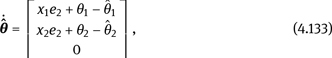

On Simulink platform, we set the unknown parameter c = 5. It means the true value of the estimated parameter is θ = δ = [0,4, 5]T. If the initial conditions of the synchronization system are X(0) = [4.4356, 6.1771, 7.2330]T, Y(0) = [–0.5431, 0.0995, –2.8096]T, ![]() (0) = [–1, –1, 0]T, δ̂(0) = [–2, –2, 0]T, respectively, and d1 = d2 = d3 = 5, we obtain the synchronization error curves, attractors, and error curves of the estimated parameters as shown in Figure 4.38. Figure 4.38(a) shows that the two chaotic systems with different initial values and unknown parameters can achieve the function projective synchronization in about 2.5 s, and it has oscillation attenuation characteristic. Figure 4.38(b) shows that the attractor of the response system and drive system is inverse, and the size ratio satisfies the projective function. From Figure 4.38(c) and (d), it can be seen that in a short time, the error of the estimated parameters θ̂1, θ̂2 and δ̂̇1, δ̂̇2 converges to zero, which indicates that the unknown parameters are identified. The results also show that the larger the control parameter di is, the better the synchronization performance is, which is important for secure communication application.
(0) = [–1, –1, 0]T, δ̂(0) = [–2, –2, 0]T, respectively, and d1 = d2 = d3 = 5, we obtain the synchronization error curves, attractors, and error curves of the estimated parameters as shown in Figure 4.38. Figure 4.38(a) shows that the two chaotic systems with different initial values and unknown parameters can achieve the function projective synchronization in about 2.5 s, and it has oscillation attenuation characteristic. Figure 4.38(b) shows that the attractor of the response system and drive system is inverse, and the size ratio satisfies the projective function. From Figure 4.38(c) and (d), it can be seen that in a short time, the error of the estimated parameters θ̂1, θ̂2 and δ̂̇1, δ̂̇2 converges to zero, which indicates that the unknown parameters are identified. The results also show that the larger the control parameter di is, the better the synchronization performance is, which is important for secure communication application.

Figure 4.38: Projective synchronization between systems (4.130) and (4.131); (a) synchronization error curve; (b) attractors; (c) error curves for estimated parameters ^θ1 and θ̂2; and (d) error curves for estimated parameters δ̂1 and δ̂2.
4.9.3.3Synchronization Control and Simulation of Heterogeneous Chaotic Systems with Unknown Parameters
Applying the adaptive function projective synchronization method to the simplified Lorenz system and Chen system with unknown parameters, the drive system and the response system are, respectively,


where θ = [θ1, θ2, θ3]T and δ = [δ1, δ2, δ3]T are the unknown parameters of the two systems, and U = [u1, u2, u3]T is the nonlinear controller. If we set the projective function as Φ(t) = –3 + 2 sin(t), according to Theorem 4.11, the control law and parameter adaptive law of the synchronization system are


For simulation, we set the unknown parameter of the simplified Lorenz system c = 5, which means that the true value of the estimated parameter is θ = [0,4,5]T. At the same time, we choose the true value of the unknown parameter of the Chen system δ = [25, 28, 1/3]T. If the initial conditions of the system and unknown parameter are X(0) = [4.4356, 6.1771, 7.2330]T, Y(0) = [–0.62, –0.4261, –4.0838]T, θ̂(0) = [–1, –1, 0]T, δ(0) 2, 2, 2]T, and d1 d2 d3 5, then we obtain the synchronization error curves, attractors, and error curves of the estimated parameters as shown in Figure 4.39. Figure 4.39(a) shows that the two chaotic systems with different initial values and unknown parameters can achieve the function projective synchronization in about 2 s, and it has oscillation attenuation characteristic. Figure 4.39(b) shows that the attractor of the response system and drive system is inverse phase, and the size ratio satisfies the projective function. From Figure 4.39(c) and (d), we know that in a short time, the error of the estimated parameters θ̂1, θ̂2 and δ̂̇1, δ̂̇2, δ̂̇3 converges to zero, which indicates the unknown parameters are identified. The results also show that the larger the control parameter di is, the better the synchronization performance is. That is, the setup time of the synchronization is shorter.

Figure 4.39: Projective synchronization between systems (4.135) and (4.136): (a) synchronization error curve; (b) attractors; (c) error curves for estimated parameters θ̂and θ̂2; and (d) error curves for 1 estimated parameters δ̂1, δ̂2, and δ̂3.
4.10Problems and Development of Chaos Synchronization
Combining with the new control strategies or dynamic methods, how to improve the performance of chaotic synchronization is key for the application research of chaos. Under the condition of noise interference, channel distortion, and parameter mismatch, the synchronization performance improvement of chaotic system is an important part of the research of chaos synchronization. In terms of the current research of chaos synchronization, we should combine the robust method of control and the stability of dynamics to improve the robustness and the synchronization performance of the synchronization system.
We should pay more attention on the problem of hyperchaos synchronization, because the secure communication based on hyperchaotic system has better security performance. For example, hyperchaos system is a high-dimensional strange attractor in the appropriate regression map. The modulated signal and the original chaotic signal are mixed together, and it cannot be resolved, so it is difficult to decryption. At present, the research on the hyperchaotic system and its synchronization is still in the early stage. The difficulties and hot topics in the research of chaos synchronization theory include the criteria, the physical mechanism, and the applications of the hyperchaotic synchronization.
It is very important to study the effects of noise interference and channel distortion on synchronization. In the real transmission process, the chaotic signal is inevitably subject to noise interference. In addition, any transmission channel is not ideal. So the transmitted signal will have amplitude attenuation, phase, and nonlinear distortion. This will inevitably have a direct or indirect effect on the synchronization of chaotic systems. It is very important to develop such kind of research for the application of chaotic synchronization in secure communication.
Although chaos synchronization control method has been studied for more than 30 years, and a lot of physics and information scientists have done a lot of work in both theory and experiment, it is still in the exploratory stage. We believe many problems such as synchronization mechanism, anti-interference ability, and so on will be solved in the future.
Questions
- What are the performance index of chaotic synchronization system and its significance?
- What are the criteria or guidelines for synchronization of chaotic systems?
- What are the key issues and challenges facing the chaos synchronization?
- Try to construct a chaotic synchronization system and analyze its synchronization performances by simulation.