
9
Photoelasticity
9.1 INTRODUCTION
Photoelasticity is a whole field stress analysis technique using the relative retardation between two components of a light vector along the directions of two principal stresses at a point on a photoelastic model. A photoelastic model is a transparent material possessing the property of birefringence (or temporary double refraction). Without external load, the model is optically isotropic and when it is loaded, refractive index changes along the directions of principal stresses in the model. Difference in refractive index along two directions measured through a monochromatic light vector is proportional to the difference in principal stresses at the point. In photoelasticity the difference of principal stresses is measured through the phase difference between two components of a light vector using a plane polarized light or a circularly polarized light.
Through photoelasticity we study the isochromatic fringes formed when viewed through an analyzer of an optical arrangement and fringe order at a particular point is proportional to the difference of principal stresses at the point. Then there are compensation techniques to know the exact fringe order at the point of interest and there are separation techniques to separate the two principal stresses.
Study of stresses in a prototype is made through a photoelastic model. Model is calibrated for stress fringe value. Then stresses from model to prototype are converted using a scaling technique.
9.2 STRESS OPTIC LAW
There are many transparent, non-crystalline materials which are optically isotropic when free of stress but become optically anisotropic after the application of stress. This behaviour is known as double refraction and the materials exhibiting this behaviour are known as photoelastic materials. As long as the loads are maintained on a photoelastic material, it exhibits the behaviour of temporary double refraction and the material becomes again isotropic after the removal of the load. Sir David Brewster observed this behaviour of double refraction in 1816.
Figure 9.1 shows an unstressed thin disc of a photoelastic material. The refractive index of this material in any direction is n0. This thin disc is subjected to loads such that the principal stresses developed at a point O are p1 and p2 as shown in Figure 9.2. The refractive index of the material changes to n1 in the direction of p1 and to n2 in the direction of p2. These changes in the indices of refraction of a material exhibiting double refraction or birefringence can be related to the state of stress in the material. Maxwell in 1853 observed that these changes in refractive indices are linearly proportional to the stresses.
|
n1 − n0 = c1 p1 + c2 p2 |
(9.1) |
|
n2 − n0 = c1 p2 + c2 p1 |
(9.2) |
where p1, p2 are the principal stresses at a point in a material under plane stress condition; n0 refractive index of unstressed material; n1, n2 indices of refraction of the material in the stressed state associated with the directions of principal stresses p1 and p2; and c1, c2 stress optic coefficients.
These changes in index of refraction can be used as the basis for a stress measurement technique, i.e. photoelasticity.
where c2 – c1 = c, relative stress optic coefficients in terms of Brewster
If p1 > p2 and the velocity of propagation of the light wave associated with principal stress p1 is greater than the velocity of propagation of light wave associated with principal stress p2, then it is known as positive birefringence.
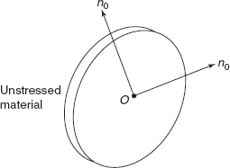
Figure 9.1 Optically isotropic thin disc
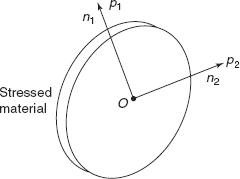
Figure 9.2 Optically anisotropic thin disc
A photoelastic model behaves like a wave plate and it can be used to relate the relative angular phase shift δ (or relative retardation) to the changes in the indices of refraction in the material due to stresses. If a beam of plane polarized light is passed through the thin sheet of photoelastic material at normal incidence as shown in Figure 9.3, then relative retardation, δ, between the two components of the light vector along each of the principal stress directions can be obtained by
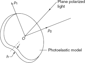
Figure 9.3 Plane polarized light vector passing through model
where h = thickness of the model, and
δ = magnitude of the relative angular phase shift developed between two components of light beam propagating in directions, perpendicular to p1 and to p2.
The component associated with the principal stress p1 will propagate at a velocity V1 which is higher than the velocity V2 of the component associated with the principal stress p2, if p1 > p2.
Equation (9.4) shows that relative retardation, δ, is linearly proportional to (i) (p1 − p2), (ii) h, and inversely proportional to the wavelength λ of the light being used.
The relative stress optic coefficient c is assumed as a material constant. Eq. (9.4) can be written as
where ![]() the relative retardation in terms of complete cycle, and
the relative retardation in terms of complete cycle, and ![]() = stress fringe value.
= stress fringe value.
Stress fringe value is a property of the model material and is determined by calibration. λ is the wavelength of light and obviously a light of single wave length or monochromatic light should be used in the study of photoelastic behaviour of a model.
If a photoelastic model material exhibits a perfectly linear elastic behaviour, the difference in principal strains (ε1 − ε2) can also be measured by establishing the value of N, relative retardation.
Now,
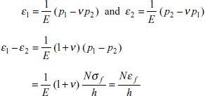
or
where εf is the material fringe value in terms of strain. If the behaviour of the material is linearly elastic, then the determination of N is sufficient to know principal stresses difference (p1–p2) or principal strains difference(ε1–ε2). But many photoelastic materials exhibit viscoelastic properties and Eq. (9.6) will not be valid in such cases.
Calibration of a photoelastic model for stress fringe value will be discussed in Chapter 13 on experiments where in a circular disc of known dimensions, subjected to known load is observed for isochromatic fringes. Knowing the stresses at the centre of the disc and fringe order at the centre of the disc, a calibration curve is plotted and σf is determined.
9.3 PROPERTIES OF LIGHT
The colour of the visible light is determined by the frequency of the components of the light vector. The colours in the visible spectrum range from deep red to deep violet with frequencies of 390 × 1012 Hz to 770 × 1012 Hz, respectively. Most photoelastic studies are made by using light in the visible range.
When the light vector is composed of vibrations, all of them having the same frequency, it is called monochromatic light, i.e. light of single colour. When the components of the light vector are of different frequencies, the colours of all the components are mixed and eye records this mixture as white light.
Ordinary light consists of electromagnetic waves vibrating in directions perpendicular to the direction of propagation. When the vibration pattern of these waves exhibits a preference as to the transverse direction of vibration, then the light is said to be polarized. Two types of light, i.e. (i) plane polarized and (ii) circularly polarized light, are used in photoelasticity.
Plane polarized light is obtained by restricting the light vector to vibrate in a single plane known as the plane of polarization. Figure 9.4 shows that the tip of the light vector sweeps out a sine curve as it propagates. The light is vibrating in the plane of polarization.
Plane polarizers are optical elements which absorb the components of the light vector not vibrating in the direction of the axis of the polarizer. When a light vector passes through a plane polarizer, this optical element absorbs that component of the light vector which is perpendicular to the axis of polarization and transmits the component parallel to the axis of polarization as shown in Figure 9.5. Say the light vector A = a sin ωt where a = amplitude and ω = frequency of light wave, and α = angle which the light vector A makes with the axis of polarization. Then
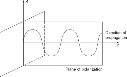
Figure 9.4 Plane of polarization
A0 = Absorbed component= a sin ωt sinα
At = Transmitted component= a sin ωt sin α cosα (9.7).
In a plane or linear polarizer, H type polaroid film is used which is a thin sheet of polyvinyl alcohol heated, stretched, and bonded to a supporting sheet of cellulose acetate butyrate. The polyvinyl face of the assembly is then stained with a liquid rich in iodine. The amount of iodine diffused into the sheet determines its quality which is judged by its transmission ratio.
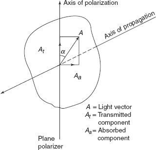
Figure 9.5 Plane polarizer
Circularly polarized light is obtained when the tip of the light vector describes a circular helix as the light propagates along the z-axis as shown in Figure 9.6. Circularly polarized light is obtained with the help of a quarter wave plate (QWP), made of a double refracting material. It resolves the light vector into two orthogonal components and transmits each of them at different velocities. The phase difference between these two components is π/2, i.e. quarter of a cycle.
The light vector component transmitted by plane polarizer is
There are two axes 1 and 2 of the QWP shown in Figure 9.7. At makes an angle β with the axis 1 of the QWP. At is resolved into two components along two axes 1 and 2, i.e. fast and slow axes of the QWP. Component At travels at a velocity V1 which is more than the velocity V2 with which the component At2 travels.
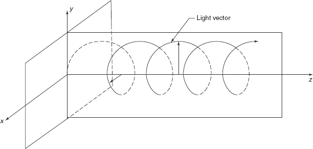
Figure 9.6 Circularly polarized light
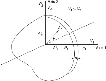
Figure 9.7 Quarter wave plate
Now
Since V1 > V2, the two components emerge from the plate with a phase difference.
Let λ = wave length of light.
Change in refractive index in direction (1)
Change in refractive index in direction (2)
Then,
Wave plates employed in a photoelastic study may consist of a single plate of quartz or calcite cut parallel to the optic axis; a single plate of mica, a sheet of oriented cellophone, or a sheet of oriented polyvinyl alcohol. QWPs are designed for a monochromatic light.
When angle β = 45° and δ = ![]() , a circularly polarized light is obtained.
, a circularly polarized light is obtained.
9.4 PLANE POLARISCOPE
A plane polariscope consists of only two linear polarizers and a light source. The polarizer nearest to the light source is called the polarizer P while the second polarizer is called the analyzer A, as shown in Figure 9.8.
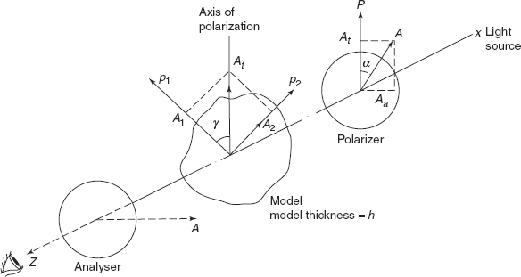
Figure 9.8 Plane polariscope
In a plane polariscope the axes of the two polarizers are always crossed and so no light is transmitted through the analyzer, and a dark field is produced. In operation, a photoelastic model is inserted between the two crossed polarizers and viewed through the analyzer. The difference of principal stresses (p1 – p2) can be measured if the fringe order N is determined. Say the direction of principal stress p1 makes an angle γ with the axis of polarization of the polarizer P. The component of the light vector transmitted by polarizer
|
At = α sin ωt cos α = α1 sin ωt, |
(9.10) |
where |
α1 = α cos α |
|
This light vector when incident on the model is resolved into two components along principal stress directions, i.e.
|
A1 = At cos γ = α1 sin ωt cos γ |
|
|
A2 = At sin γ = α1 sin ωt sin γ |
(9.11) |
A1 and A2 are incident on one side of the photoelastic model. These two components of the light vector propagate through the stressed model at different velocities. As a result, when these two components emerge from the model, these are out of phase. Say the relative phase difference between the two components is δ.
Then
If this relative phase difference is divided equally between the two components, then the two components emerging from the model will become
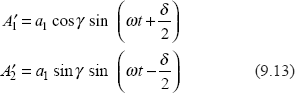
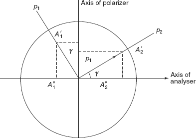
Figure 9.9 Crossed polarizer and analyzer
These two light vector components emerging from the model reach the analyzer. But analyzer and polarizer are crossed, so if the axis of polarizer is vertical, then axis of analyzer will be horizontal as shown in Figure 9.9. Components ![]() and
and ![]() transmitted by the analyzer, respectively, are
transmitted by the analyzer, respectively, are
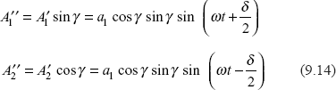
Net light vector transmitted by the analyzer
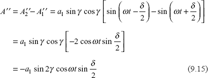
The intensity of light, as recorded by the eye is proportional to the square of the amplitude of the light vector emerging from the analyzer.
So,
Intensity of light, |
I = 0 if cos ωt = 0 |
|
|
|
|
These are summarized as follows:
- Frequency effects Circular frequency of light, ω, is of very higher order. Therefore, eye or any type of available high speed photographic camera equipment does not record the periodic extinction when cos ωt becomes zero.
- Effects of Principal stress-directions The intensity I becomes zero when 2γ = 0 or when
sin 2γ = sin nπ
or
2γ = nπ
where n = 0, 1, 2, 3, 4, …
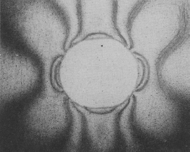
or when the principal stresses are aligned along the axes of polarizer and analyzer, the extinction will occur. All the points on the model can be determined where extinction occurs. When the entire model is viewed through the analyzer, a fringe pattern is observed. These fringes are loci of points where the principal stress directions (p1 or p2) coincide with the axis of polarizer. These fringes produced by sin22γ = 0 term are known as Isoclinic fringes.
- Effects of principal stresses difference
Intensity, I = 0, when sin
 = 0
= 0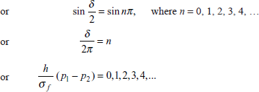
The order of the extinction is controlled by the magnitude of the difference of principal stresses. The fringe pattern related to the principal stresses difference is called Isochromatic fringe pattern.
These two sets of extinction lines called isoclinic and isochromatic fringes are superimposed upon one another. When a monochromatic light source is used, both the fringes appear dark. But when white light (ordinary light) source is used, isochromatic fringes appear coloured and isoclinic fringes appear dark.
9.5 PROPERTIES OF ISOCLINIC FRINGES
Isoclinic fringes for a particular model can be obtained for various values of the angle γ, i.e. the angle between the direction of one principal stress and the axis of the polarizer. While sketching the composite isoclinic pattern, following rules should be followed.
- Isoclinics of all parameters must pass through the singular or isotropic points. These are the points where principal stresses, p1 = p2, so that the fringe order remains zero, as shown in Figure 9.10 (a). A and B are singular points for a circular ring under diametral compression.
- Isoclinic of one parameter must coincide with an axis of symmetry in the model, if the axis of symmetry exists. In Figure 9.10 (a), vertical diameter CD is the axis of symmetry.
- The parameter of an isoclinic intersecting a free boundary can be determined by the slope of the boundary at the point of intersection.
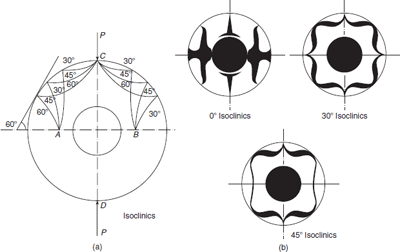
Figure 9.10 Isoclinics of different parameters
- Isoclinics of all parameters must pass through the points of application of the concentrated load such as points C and δ in Figure 9.10(a).
Figure 9.10(b) shows 0°, 30°, 45° isoclinic parameters for a ring under diametral compression. Note that these isoclinic fringes are not sharp lines but they are a bunch of considerable thickness.
9.6 CIRCULAR POLARISCOPE
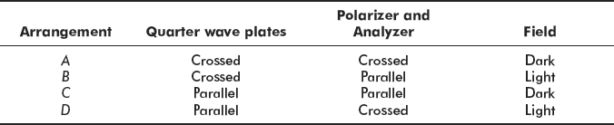
A circular polariscope employs a circularly polarized light and consists of four elements and a light source. Polarizer, P, converts ordinary light into plane polarized light. First QWP converts this plane polarized light into a circularly polarized light if angle β = π/4 The QWP has fast and slow axes as shown in Figure 9.11. The second QWP is set with its fast, F-axis parallel to the slow S, axis of the I QWP. The second QWP converts the circularly polarized light into the plane polarized light again. The purpose of analyzer, A, after the II QWP is to extinguish the light vector. The axis of analyzer is crossed with the axis of the polarizer. This series of elements P, I QWP, II QWP, and A constitutes the standard arrangement for a circular polariscope and this particular arrangement produces dark field. Four optical arrangements are possible with these elements depending upon whether the polarizer and analyzer, I and II, QWPs are crossed or parallel to each other. These arrangements are tabulated in Table 9.1.
Arrangements A and B are normally recommended for light and dark field usage of polariscope since a portion of error introduced by imperfect QWPs is cancelled out.
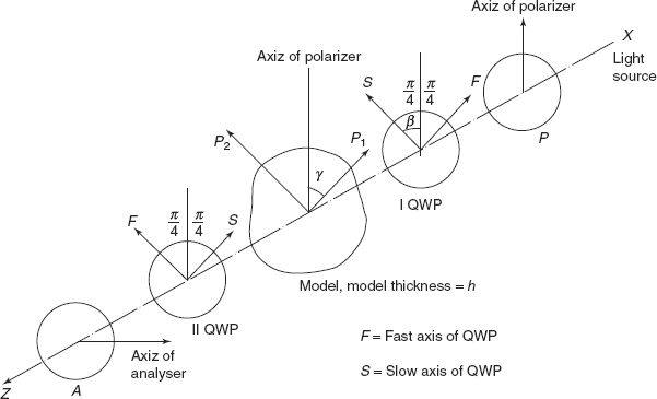
Figure 9.11 Circular polariscope (dark field arrangement)
Table 9.1 Optical arrangements of a circular polariscope
Dark Field Arrangement Now a stressed photoelastic model is placed in the field of circular polariscope with its normal coincident with the z-axis of polariscope shown in Figure 9.11.
The plane polarized light beam emerging from the polarizer is
As the light enters the 1st QWP it is resolved into two components Af and As, along fast and slow axes of QWP.
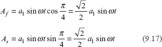
When these two light vectors emerge out from the I QWP, there will be phase shift of π/2 between them, the emerged components will be
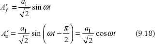
These components represent circularly polarized light. After leaving the I QWP, the components enter the model, which exhibits the characteristics of a temporary wave plate. The two components ![]() are resolved into two components A1 and A2 along the directions of principal stresses p1 and p2. Say the stress p1 is inclined at an angle γ to the axis of polarizer, then
are resolved into two components A1 and A2 along the directions of principal stresses p1 and p2. Say the stress p1 is inclined at an angle γ to the axis of polarizer, then
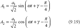
These two components propagate through the model with different velocities. The additional relative retardation δ accumulated during propagation through the model is given as
The waves upon emerging from the model can be expressed as
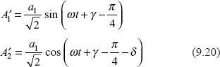
The light emerging from the model propagates to the second QWP and is resolved into two components along fast and slow axes of 2nd QWP. When these two components emerge from the II QWP, there will be phase difference of ![]() between the two components. Finally the light enters the analyzer. The component of light vector transmitted by the analyzer will be
between the two components. Finally the light enters the analyzer. The component of light vector transmitted by the analyzer will be
The intensity of light being proportional to the square of the amplitude of the light wave emerging from the analyzer is given by
Now,
These frequency effects involving the effect of ω cannot be recorded by eye or by any high speed photographic camera. Moreover, in this equation angle γ is associated with frequency ω, therefore, isoclinic fringes do not appear.
Secondly
or
or
The loci of these points of extinction produce a pattern known as Isochromatic fringes same as obtained by using a plane polariscope. Order of fringes will be 0, 1, 2, 3, 4,… in this dark field arrangement.
Light field arrangement In the light field circular polariscope, the orientation of the four optical elements, i.e. polarizer, I QWP, II QWP, and analyzer is shown in Figure 9.12, where polarizer and analyzer are parallel and two QW plates are crossed. The light vector emerging from the analyzer, At = a1 sinωt passes through the I QWP, stressed model, II QWP, and finally the analyzer. The amplitude of the component of the light emerging from the analyzer will be
The intensity of the light vector emerging from analyzer is
Now I = 0 if cos ωt = 0
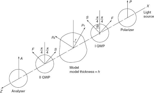
Figure 9.12 Circular polariscope (light field arrangement)
This frequency effect involving the effect of ω cannot be recorded by eye or by any high speed photographic camera because ω is very high, i.e. of the order of 105 cps.
Moreover,
or
or
Obviously the order of the first fringe observed in a light field circular polariscope is ½. These fringes are known as Isochromatic fringes. Again the isoclinic fringes are eliminated even in light field arrangement of circular polariscope.
9.7 COMPENSATION TECHNIQUES
We have learnt so far that there are two types of fringes viewed through the analyzer, i.e.
- Isoclinic fringes.
- Isochromatic fringes.
Isoclinic fringes are the loci of points where the principal stress directions (of p1 or of p2) coincide with the axis of polarizer.
Isochromatic fringes or the order of isochromatic fringes is related to the principal stresses difference, i.e. (p1 – p2). In plane polariscope the order of isochromatic fringes is 0, 1, 2, 3, …, n. In circular polariscope the order of fringes in dark field arrangement is 0, 1, 2, 3, …, n, while the order of fringes in light field arrangement is 0.5, 1.5, 2.5, …, (n – 0.5).
If we superimpose the photographs of isochromatic fringes obtained from dark field and light field arrangements of circular polariscope then we will have fringe order as 0, 0.5, 1.0, 1.5, 2.0, 2.5, …, (n).
By interpolation between the fringes, one can estimate the order of fringe up to ±0.1, which results in the accuracy for the measurement of principal stress difference of ±0.1σf/h where σf is stress fringe value and h is the model thickness.
However, to know the exact fractional fringe order at the point of interest there are two methods of compensation available, i.e. (i) Tardy’s method and (ii) Babinet Soleil method.
9.7.1 Tardy’s Method
In Tardy’s method of compensation, following is the procedure to get fractional fringe order at the point of interest on model.
- A plane polariscope is made.
- Model is loaded with external load.
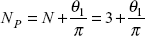
- Polarizer and analyzer are simultaneously rotated so that a particular isoclinic passes through the point of interest. Figure 9.13 shows a photoelastic model, with isoclinics of 10°, 20°, 30°, and 20° isoclinic passes through the point of interest P. Note that isoclinic fringes are not sharp lines but these are bands of considerable width.
- Now keeping the position of Polarizer and Analyzer as fixed, QWPs are rotated so as to get dark field arrangement of circular polariscope and only isochromatic fringes are observed through the analyzer, and isoclinic fringes vanish (do not appear in circular polariscopic arrangement).
- Point P lies in between the isochromatic fringes of orders 3 and 4. The exact fringe order lies between 3 and 4.
- Now the analyzer is decoupled from polarizer and the analyzer is rotated through an angle θ1, such that 3rd order fringe moves towards point P and coincides with P. Then fringe order at P
Note that point P is closer to fringe order 3.
- If the point P is closer to isochromatic fringe of order 4, then analyzer is rotated in a negative direction by angle θ2 so that fringe order 4 moves towards the point P and finally coincides with the point P, then exact fringe order at point P
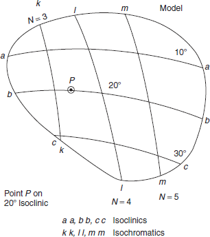
Figure 9.13 Photoelastic model with various isoclinics

This method is very fast and effective provided the isoclinic parameters are used accurately to determine principal stress direction at the point of interest. By accurate measurements, fringe order up to two decimal places is determined by the method.
9.7.2 Babinet Soleil Method
This compensator employs a plate and a wedge of quartz, which is permanently doubly refractive (birefrigent). The photoelastic model is temporarily doubly refractive due to the application of load. The optical effect of the superposition of these two effects is shown in Figure 9.14.
Compensator consists of a quartz plate of uniform thickness t1 and a wedge of quartz of variable thickness t2. Optical axis of plate of uniform thickness and the wedge are perpendicular to each other.
Procedure is as follows:
- Point of interest is selected on model.
- Isoclinic parameters are established at this point of interest and direction of principal stresses p1 and p2 are known.
- Compensator is aligned with its axis parallel to principal stress p2.
- Now the wedge thickness is varied, or birefringence of compensator is equal to (p1 – p2).
- Combined fringe order becomes zero as shown.
- N exact fringe order can be determined with accuracy of three decimal places.
Figure 9.14 Babinet soleil compensator
9.8 FRINGE SHARPENING BY PARTIAL MIRRORS
D. Post has shown that bandwidth of Isochromatic fringes can be reduced with the help of partial mirrors placed parallel on both the sides of photoelastic model under load, in a circular lens type polariscope.
Ray of light emerging from partial mirror traverses the model and then passes through partial mirror as ray 1. There is loss of intensity of light as ray transmits through partial mirrors and intensity goes on reducing.
In the case of dark field arrangement of circular polariscope, the intensity of light is
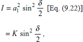
where K is constant ![]()
The intensity of ray 1 is reduced by
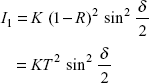
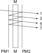
Figure 9.15 Fringe sharpening
where |
R |
= |
reflection coefficient of partial mirror, |
|
T |
= |
transmission coefficient of partial mirror, and R + T = 1. |
For ray 3, there are two reflections and two transmissions and ray traverses the model three times, the intensity of light will be
Similarly for ray numbers 5 and 7, intensity is
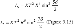
Like this intensity of light goes on reducing and the fringes become sharpened, with the result there is a variation of intensity of light from maximum to minimum, when we get minimum intensity, we get dark fringes with order 0, 1, 2, 3, … and we get maximum intensity, we get light fringes with order 0.5, 1.5, 2.5, 3.5 as shown in Figure 9.16.
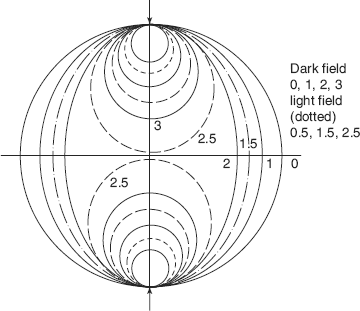
Figure 9.16 Sharpened fringes-circular disc under diametral combination
In actual practice, rays are not inclined as shown; these rays propagate back and forth through the model at the same point of the model number of times and intensity of light ray progressively diminish.
9.9 FRINGE MULTIPLICATION BY PARTIAL MIRRORS
D. Post has also shown that the partial mirrors can be used to multiply the number of isochromatic fringes if one partial mirror is placed parallel to the photoelastic model and the other partial mirror is placed slightly inclined with the plane of photoelastic model as shown in Figure 9.17. Partial mirror PM I is parallel to model M but partial mirror PM II is slightly inclined with the model at an angle α Ray 1 emerges from partial mirror II, traversing two times the partial mirrors and one time through the model, intensity of light for ray 1 is
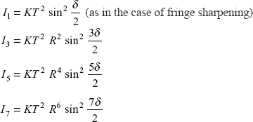
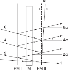
Figure 9.17.
Different rays are inclined with the axis of polariscope, at angles 0, 2α, 4α, 6α as shown, each rays gets isolated and passes out from different points of the model. Any of these rays can be observed at the proper image point of focal field lens.
As is obvious from the intensity equations above, isochromatic fringe patterns can be multiplied by 1, 3, 5, or 7 or more. Fringes are not only multiplied but they are sharpened at the same time.
Fringe order recorded with ray 1 are 0, 0.5, 1.0, 1.5, 2, 2.5, 3, … (as in fringe sharpening). Fringe order recorded with ray 3 are 0, ![]() . Similarly fringe orders recorded with ray 5 are 0.1, 0.2, 0.3, 0.4, … 1.0, etc.
. Similarly fringe orders recorded with ray 5 are 0.1, 0.2, 0.3, 0.4, … 1.0, etc.
Say the multiplication obtained by partial mirrors is 3, then fringe order recorded for a circular disc under compression will be as shown in Figure 9.18.
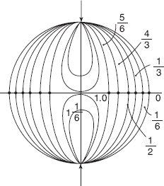
Figure 9.18 Fringe order for a circular disc under compression
9.10 SEPARATION TECHNIQUES
With the help of photoelastic analysis, we get the value of (p1 – p2), i.e. principal stresses difference from the isochromatic fringe order N, such that
There is a necessity of separating the two principal stresses p1 and p2, so that complete state of stress is known. At the free boundaries of a component the principal stress in a direction perpendicular to the free boundary is zero, so other principal stress is known through the isochromatic fringe order. But for the complete analysis, values of principal stresses in the interior of a component should also be known. For separating the two principal stresses p1 and p2 from (p1 – p2) there are several techniques, but following two techniques are commonly used due to simple operation:
- Shear difference method.
- Oblique incidence method.
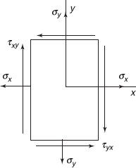
Figure 9.19 Plate under plane stress
Shear difference method is based upon the equilibrium equation as follows for the plane stress case shown in Figure 9.19
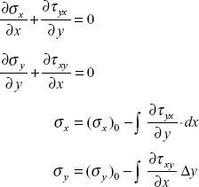
By finite differences technique
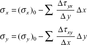
where (σx)0 and (σy)0 are known stresses at the boundary, i.e. at the starting point, for the integration process.
In the above equation, shear stress
as shown by Mohr’s stress circle in Figure 9.20. Shear stress at any interior point,
Shear stress,
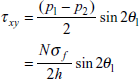
where θ1 is the orientation of principal stress p1 with respect to the plane of stress σX or θ1 is the isoclinic parameter of the point with respect to the polarizer axis.
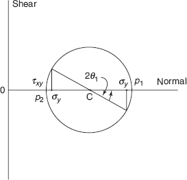
Figure 9.20 Mohr’s stress circle
The term Δτxy is determined from a plot of shear stress distribution along two auxiliary lines (parallel to the line of interest) ![]() area between the τxy curves.
area between the τxy curves.
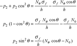
Example 9.1 Let us consider a thin rectangular plate with a central circular hole, subjected to uniformly distributed load of intensity f in y-direction under plane stress condition as shown in Figure 9.21(a). Stresses are maximum at the edge of the hole at O, along x-axis. Let us determine principal stresses along ox, starting at o, where σ1 has some value but stress σ2 is zero.
or
Similarly,
There are two auxiliary lines ab and cd parallel to ox. Let us determine τxy along ab and cd and plot as shown in Figure 9.22. The figure shows plot of τxy along ab and cd, noted through fringe order
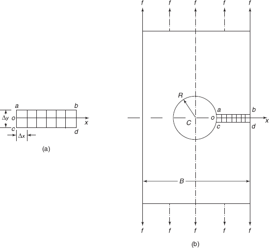
Figure 9.21 Example 9.1
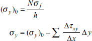
N and isoclinic parameters ![]() Once σx is known at a given point, the value of σy can be calculated from
Once σx is known at a given point, the value of σy can be calculated from
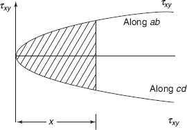
Figure 9.22 Variation of shear stress
Now
Stress invariant, p1 = (σx + σy) − p2
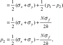
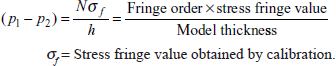
where N = fringe order, σf = stress fringe value, and h = model thickness.
Principal stresses along ox are obtained from above two expressions.
9.10.1 Oblique Incidence Method
In ordinary polariscope arrangement light is incident normal to the plane of photoelastic model and a isochromatic fringe order N0 is observed at the point of interest, and
If we know the principal stress-directions of p1 and p2 as shown in Figure 9.23, model is rotated about an axis in direction of principal stress p1 as shown in Figure 9.23.
Say the model is rotated by an angle θ as shown in Figure 9.24. The light ray passes through a distance of ![]() in the model. Fringe order Nθ is noted, in the plane containing stresses p1 and p′2 (secondary principal stress)
in the model. Fringe order Nθ is noted, in the plane containing stresses p1 and p′2 (secondary principal stress)
From theory of elasticity we know that
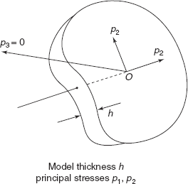
Figure 9.23 Principal stresses at point O in model
Figure 9.24 Rotation of model about an axis of principal stress p1
So,
From Eqs (9.25) and (9.26)
Principal stress,
Putting the value p2 in Eq. (9.25) and after simplification, we get
In a model under plane stress condition, the isoclinic at the point of interest can be determined and directions of principal stresses are known at the point of interest.
This oblique incidence approach is generally used to separate stresses along a line of symmetry where one rotation of the model about line of symmetry provides sufficient data for the whole line and principal stresses can be separated along whole of this line.
9.10.2 Electrical Analogy
In a uniformly electrically conducting surface enclosed by boundary which is subjected to a known potential, the Voltage Distribution is governed by Laplace Equation in the same manner as the sum of principal stresses in a plane stress state.
Say applied voltage at a point on boundary of uniformly conducting surface is V, then
V |
= |
p1 + p2 = sum of principal stresses, while in a photoelastic model |
Nσf /h |
= |
p1 − p2 = difference of principal stresses |
At the free boundary where either p1 = 0 or p2 = 0, then
Electrical model of same geometry as of photoelastic model is fabricated from a uniformly conducting paper containing uniform thin layer of fine particles of graphite. A company has marketed electrically conducting paper by trade name TELEDELTOS, with resistance values 30–120 Ω/mm2, size of paper, width 1 m and length several meters. Figure 9.25 shows a plate of width B and depth D with a central hole of diameter δ, subjected to uniform axial load as shown. A photoelastic model of this size can be analyzed for isochromatic fringes and fringe order at the points can be noted using any compensation technique.
Taking the advantage of symmetry of the model along x and y axes, only one quadrant of model is analyzed. Therefore electrical model is made as shown in Figure 9.26, with dimensions B/2 and D/2, with a quarter of hole from electrically conducting paper. Voltage of 6 volts is applied as shown and the voltage at point of interest is noted down or Isopachic lines can be plotted, i.e. lines of constant sum of principal stresses in the region marked by boundary abcde. Starting from the free boundary where one of the principal stresses is zero, or one principal stress is known from photoelastic analysis these isopachic lines can be plotted. At the boundary voltage can be simulated to the applied stress.
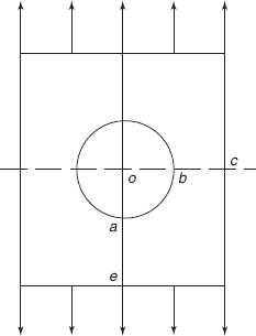
Figure 9.25 Photoelastic model
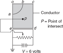
Figure 9.26 Electrical model
At any given point sum of principal stresses is known from isopachic lines (from electrical model) and difference of principal stresses is known from isochromatic fringe value (from photoelastic model) or taking into account the stress fringe value of the material principal stresses at any point can be determined.
9.11 STRESSES IN PROTOTYPE
In photoelasticity, stresses are analyzed in a polymeric photoelastic material but prototypes are generally made of metals. Therefore, stresses obtained in a photoelastic model are converted into stresses that would occur in a prototype. If the study is made on a model under plane stress or plane strain conditions, then there is no effect of Young’s modulus of the material on the stress distribution in model due to external loads. Moreover if (a) body forces are absent or (b) body forces are constant as gravitational forces or (c) body forces vary linearly along the dimension of the model, then there is no effect of Poisson’s ratio of the material on the stress distribution. However, to take the advantage of similarities between model and prototype, there are two conditions to be satisfied, i.e.
- body is simply connected, i.e. there are no series of holes in model or prototype.
- there is no distortion in model at the root of a notch, a keyway, etc. However, to minimize the effect of distortion, photoelastic material with high figure of merit should be taken. Figure of merit is a ratio of E/σf i.e. ratio of Young’s modulus of elasticity/stress fringe value.
If these conditions are satisfied, the principle of similitude between model and prototype can be used.
Stress in prototype,
where |
σm = stress in model, |
|
Pp = load on prototype, |
|
Pm = load on model, |
|
hm = thickness of model, |
|
hp = thickness of prototype, |
|
lm = typical length of model, and |
|
lp = typical length of prototype. |
Similarly displacement in prototype,
where Em = Young’s modulus of model, and
Ep = Young’s modulus of prototype.
9.12 THREE DIMENSIONAL PHOTOELASTICITY
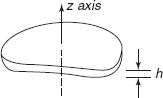
A three dimensional model of a photoelastic material is made and stresses due to external load are locked in the model during a stress–freezing process. After the completion of stress process, the model is cut into thin slices and interior region of the model is photoelastically analyzed.
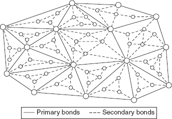
Figure 9.27 Primary and secondary bonds
Some polymeric materials exhibit di-phase behavior, i.e.
- molecular chains are well boned in a three dimensional network of primary bonds (having longer molecules chains),
- a large number of molecules are less solidly bonded by secondary bonds (having shorter molecular chains) as shown in Figure 9.27.
At room temperature, both sets of molecular bonds, i.e. primary and secondary bonds resist external load. Photoelastic model (made of polymeric material) is now loaded and its temperature is raised. At a critical temperature, the shorter secondary bonds are broken but longer primary bonds remain intact and carry the entire external load.
Deformations caused by the external load are locked in the secondary bonds. Now the model is cooled to room temperature, the secondary bonds are reformed again between the deformed primary bonds and these secondary bonds serve to lock the deformations (stresses) in these deformed primary bonds.
After the load is removed, the primary bonds are relaxed by a small amount at the large part of deformation is not recovered. So, the elastic deformation in the body is permanently locked into the model by reformed secondary bonds.
9.12.1 Stress Optic Law
Say at a particular point of a three dimensional photoelastic model, the principal stresses are p1, p2 p3 respectively. If n0 is the refractive index of unstressed photoelastic model, then refractive index changes to n1, n2, n3 respectively along three principal stress directions,
such that |
n1 − n2 = c1p1 − c2 (p2 + p3) |
(9.27) |
|
n2 − n3 = c1p2 − c2 (p1 + p3) |
(9.28) |
|
n3 − n1 = c1p3 − c2 (p1 + p2) |
(9.29) |
where c1 = direct stress optic co-efficient, and
c2 = transverse stress optic coefficient.
From the above equations
where τ1, τ2, τ3 are principal shears at the point.
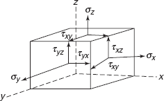
Figure 9.28 Stress Tensor
9.12.2 Secondary Principal Stresses
Stress tensor (stresses at a point) is shown in Figure 9.28.
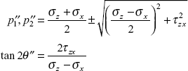
If the light is incident along z-axis, σx, σy, τxy in plane stresses, then secondary principal stresses will be
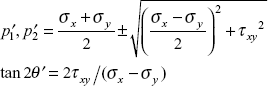
θ′ and ![]() , are orientations of the secondary principal stresses with reference to x-axis.
, are orientations of the secondary principal stresses with reference to x-axis.
If Mohr’s stress circle is drawn, then
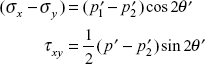
Figure 9.29 Light incident along z-axis
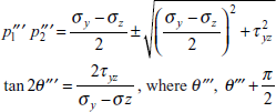
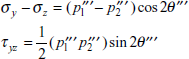
Similarly for the light incident along y-axis, secondary principal stresses are
θ″, ![]() are orientations of
are orientations of ![]() with respect to z-axis.
with respect to z-axis.
Finally if the light is incident along x-axis, the secondary principal stresses in z-y plane will be
are orientations of ![]() with respect to y-axis, or in terms of Mohr’s stress circle
with respect to y-axis, or in terms of Mohr’s stress circle
9.12.3 Photoelastic Analysis of a Slice Cut from a Model
Say the light is incident along z-axis a shown below. Light is incident perpendicular to x-y plane, ![]() where N is isochromatic fringe order, h is path traveled by light vector along z-direction, σf is stress fringe value of the material.
where N is isochromatic fringe order, h is path traveled by light vector along z-direction, σf is stress fringe value of the material.
If the light is incident obliquely then, ![]() where N’ is the isochromatic fringe order, h´ is the path traveled by light vector in oblique direction.
where N’ is the isochromatic fringe order, h´ is the path traveled by light vector in oblique direction.
Noting down the fringe order in normal and oblique incidences, the isoclinic parameter at the point of interest, stresses in cut slice can be determined.
9.13 CHARACTERISTICS OF A GOOD PHOTOELASTIC MATERIAL
A good photoelastic material should possess the following optical, physical, and mechanical properties:
- Material should be transparent to the monochromatic light employed.
- Material should have low σf, stress fringe value, and low εf, strain fringe value.
- It should possess linear σ − ε (stress–strain), σ − σf (stress vs. stress fringe value), ε − εf (strain vs. strain fringe value).
- Material should possess optical and mechanical isotropy.
- Material should be homogeneous throughout.
- Material should have high E, Young’s modulus, and high σe, elastic limit stress.
- Material should possess stable constant σf, stress fringe value, and constant εf, strain fringe value.
- Material should not creep under load.
- Material should be free from residual stresses after the model is machined to required size and dimensions.
- Material should not be very costly, and it should be available in market.
Some of the generally used photoelastic material are:
- Columbia Resin CR-39.
- Homalite 100.
- Polycarbonate.
- Epoxy most commonly used.
- Urethane rubber has very low E, and is highly sensitive, even a slight thumb pressure produces large number of fringes.
MULTIPLE CHOICE QUESTIONS
- Ratio of stress fringe value/strain fringe value is


- None of these
- Stress fringe value σf is given by


- None of these
where c = Relative stress optic coefficient,
λ = Wavelength of light, and
h = Model thickness.
- At the isotropic point, which statement is correct.
- Principal stresses are equal and opposite
- Shear stress is constant
- Principal stress difference is zero
- None of these
- Angle between plane of polarization and plane of fast axis of quarter wave plate in a circular polariscope is
- 0°
- 45°
- 7.5°
- None of these
- What are isoclinic fringes?
- Where the difference of principal stresses is proportional to phase difference between the light coming out from fast and slow axes of model
- These are the loci of points where principal stress direction (of p1 or p2) coincides with the axes of polarizer
- Neither (a) nor (b)
- Both (a) and (b)
- Tardy’s method is used as a
- separation technique
- compensation technique
- fringe sharpening technique
- None of these
- Which of the following is a permanently doubly refracting material?
- Quartz
- Epoxy
- Urethane rubber
- None of these
- By fringe multiplication technique, multiplication factor is 3, what is the order of fringes obtained?

- 0, 0.5, 1.0, 1.5
- None of these
Answers
1. (a) |
2. (b) |
3. (c) |
4. (b) |
5. (b) |
6. (b) |
7. (a) |
8. (b). |
|
|
PRACTICE PROBLEMS
9.1. Define the following:
- birefringence
- stress optic law
- stress fringe value
- strain fringe value
9.2. Explain the procedure to make plane polariscope. What is the difference between Isoclinic and Isochromatic fringes?
9.3. Explain how circularly polarized light is obtained with the help of a polarizer and a quarter wave plate.
9.4. Write down the properties of isoclinic parameters, explain with the help of a neat sketch on a circular ring under compression, sketch 0° and 45° isoclinics.
9.5. What is a light field arrangement of a circular poloriscope? What type of fringes and of what order are obtained by this arrangement? Why isoclinics are absent from this arrangement?
9.6. Explain the Babinet Soleil method of compensation with the help of a neat sketch.
9.7. Explain the fringe sharpening and fringe multiplication with the help of partial mirrors.
9.8. What are separation techniques? Explain shear difference method.
9.9. If a particular point in a photoelastic model is examined in a polariscope with a mercury light source (λ = 548 nm) and a fringe order of 3 is established, what fringe order will be obtained if a sodium light source (λ = 590 nm) were used in place of mercury source.
Ans. [2.786].
9.10. Given a fringes order of 4.5, a model thickness of 6 mm, a material fringe value of 16 kN/m, and an isoclinic parameter of 30° defining the angle between the x-axis and principal stress p1, determine shear stress τxy.
Ans. [5.2 N/mm2].