
B.2 Assemblers
Jobs to be done by an assembler: An assembler has to do the following at the minimum:
- Scan the input assembly language code, check that only valid characterset is used and statement constructs are valid.
- Replace all mnemonic op-codes by correct machine op-codes.
- Replace all symbolic addresses, address constants, etc. by proper numeric values.
- Assign data areas and provide for loading-defined data wherever specified.
- Execute all the other pseudo-operations.
We shall now consider various types of assemblers and their major characteristics. We then discuss working of a two-pass assembler for the example assembly language.
Types of Assemblers
- Line-by-line assembler: This type of assembler is usually used in debuggers, where the test engineers may like to place short code segments in a program being debugged. Only mnemonic op-codes are provided. Address are all numeric. No symbol table is created or looked up. We shall not discuss this type of assembler further.
- One-pass assembler: The assembler scans through the assembly source code only once and is expected to assemble the program during that single pass.
- Two-pass assembler: The assembler scans through the complete source code two times. During the first pass, a Symbol Table is builtup and during the second pass actual assembly of each instruction takes place, using the Symbol Table to provide address equivalents for the symbols.
- Macro assembler: An assembler which handles macros also. We discuss macros and macro assembler in Section B.2.4.
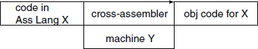
- Cross-assembler: The assembler which run on a machine other than the one for which it assemble the object program (see Fig. B.2).
B.2.1 One-pass Assembler
Such an assembler basically cannot handle forward references. For example, consider the code:
DCR      B
          JZ	FRWRD
          ...	...
          ...	...
FRWRD:    ...	...
Here, the one-pass assembler will not have address for label FRWRD and so will not be able to assemble the JZ instruction. There are three options for such an assembler:
- Forbid the programmer from using a forward reference. This of course cripples the language and is not an acceptable option.
- While reading the source code, go on storing the statements on a secondary storage unit like disc or tape. During a later phase during which the forward references can be resolved, read the source from this saved copy. This option, actually is a two-pass assembler, is disguise and is irrelevant in modern days, where fast hard discs are almost a standard feature of a general-purpose computer.
- If a forward reference is found, add a node to a ‘ToDereference’ array of linked list, where each array element has a structure:
<symbol> <address> <ptr> ––> <obj code pos #1> <obj code pos #2> …When a forward reference is not yet defined, <address> is zero. When it gets defined later in the code, the assembler inserts its address value at the code positions according to the link list. This assumes that either the complete object code is held in memory or a “random-load” loader is required.
Such an one-pass assembler was relevant when in old days the secondary storage units were slow and expensive. Sometimes it is used as back-end of a compiler, which maintains its own symbol table, though the tendency is to use a “standard” two-pass assembler even there.
We shall not discuss one-pass assembler any further.
B.2.2 Two-pass Assembler
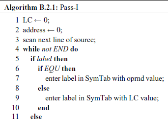
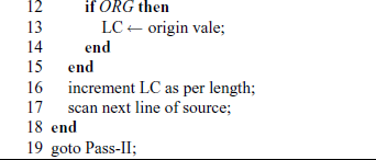
The assembler has two passes or scans over the input source code. During the first pass, the emphasis is on building up a symbol table apart from checking the lexical validity of the code. During the second pass, it replaces all references with their equivalent addresses or values, assembles the code and outputs it.
The assembler uses the following data structures:
- Symbol Table: The structure is:
<symbol> <value> - Op-code table: Stores the base values only for each op-code; the actual op-code may be computed using the modifiers from register value table. The structure is:
<Mnemonic> <Hex value> <no. of oprnds> <Type op1> <Type op2> <length> - Register value table: (operand modifier in general) The structure is:
<Reg name> <1st value> <2nd value> - Error Table: Error codes and corresponding legends.
The algorithms for Pass-I and Pass-II are given as Algorithms B.2.1 and B.2.2, respectively.
B.2.3 Symbol Table Handling
One of the most frequent operations and one which consumes major portion of execution time in an assembly operation is Symbol Table building and look-up. A real-life assembly language program may have hundreds or thousands of symbols in use. The data structure used to store the table and the algorithms used to access it contribute significantly to the speed of an assembler. The operations done on a symbol table are:
- insert a symbol if not already present in the table;
- look up a symbol if it is present in the table;
- look up various attributes of a symbol;
- modify attributes of a symbol;
Note that deleting a symbol is not a required operation. The data structure should be selected keeping these points in mind.
What are the possible options for the data structure? They are:
Simple array: Each entry is a (symbol, value) pair. As the array size would be limited and fixed, useful only for experimental work, because the number of symbols that can be allowed in the source will be limited by the array size. Also, if the symbol names are stored directly in the array, there will be an upper limit on the size of the names also, considerable wastage of memory.
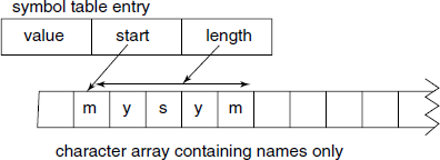
Array with pointers to symbol names: The symbol names are stored separately in a character array and within the main symbol table we put the starting index and length of the symbol name. This will allow considerable variation in the size of the symbol names, at the same time saving memory (see Fig. B.3). Even with this enhancement, the major problem of limited number of entries remains. If the implementation language is C, we can use ‘0’ terminated C strings in the name storage. This avoids storing of length value in the symbol table entry, but the implementor must take care to use the character array as readonly once a symbol name is entered in it, otherwise there is a danger of disturbing the array.
Sorted array: If the entries are put in the symbol table in an arbitrary order, then for each look-up, time O(n) will be taken, where n is the number of symbols in the table. We can sort the array every time a new symbol is inserted and use the Binary search method to look-up the table. As there is only one time insertion for each symbol, but there may be several look-ups for it, this seems to be a viable approach. As sorting does take time, one alternative is to sort the table only after 10 new symbols are inserted and use an auxiliary linked list to keep new symbols. Look-up operation checks the linked list first and then the main sorted array. When linked list has 10 symbols in it, all of them are put in the array and the array is resorted.
Linked list: If the symbol table is constructed as a singly linked list, one of the major objections to the array storage does not apply. The loop-up times will be, though, large and unacceptable for large symbol tables. One way out of this is to use multiple linked lists, one each for symbol name starting with a particular character. The link head pointers are kept in an array.
Binary search tree: Provide considerable improvement, at the cost of complexity of handling routines, over the above methods. Here, assumption is that the new symbols arrive in a random lexical order, so that the BST is more or less balanced.
Hash table: Provide possibly the best performance, especially for large source codes having thousands of symbols. Here, the main idea is that each symbol name is converted to a corresponding hash value by a fast hashing function. The hash value is a positive integer ≤ the size of the hash table. The symbol data is inserted in the hash table at that index position (see Fig. B.4).
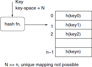
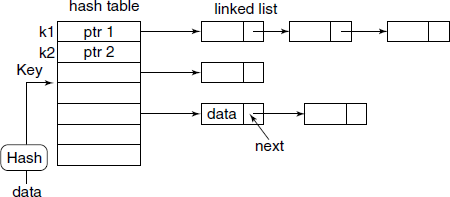
Unfortunately, the symbol name space will generally be very large compared to the number of entry slots available in the hash table. This results in what is known as collision. One of the popular methods to handle these inevitable collisions is to use linked list for each of the hash value, as shown in Fig. B.5.
B.2.4 Macro Assembler
It is usual to have a very useful facility, known as Macro facility, in an assembler. Though macro facility can be made quite complex, and many real-life assembler do have sophisticated macro facilities, even simple macro implementation can be of considerable help to an assembly language programmer.
What is a Macro?
A Macro simply means a name given to some pattern. It refers to a mapping macro : symbol ⇒ pattern. We say that the pattern defines the macro denoted by the symbol. There are two steps in using a macro: first, define a macro, by associating a symbol with an arbitrary pattern, then second, use the macro, by simply using the symbol. When we use the macro, macro expansion or replacement takes place, i.e. wherever the symbol is occurring, it is replaced by the pattern.
This simple idea of replacement of a symbol by a pattern is very powerful. It is used in assemblers, compilers, spreadsheets, text editors, etc. In fact, the software that the authors of this book used to compose it –TEX and LATEX uses macros very heavily. In Section B.3, we discuss several such macro processors.
Macros in an Assembler
An assembly language programmer finds that he uses certain sequences of assembly language statements repeatedly, with possibly minor variations.
For example, assume that adding 4 to the value of H register occurs several times in our program. We may define a macro as follows:
ADD4   MACRO
       MOV A,H
       ADI 4
       MOV H,A
       ENDM
Here, ADD4 is the name of the macro, i.e. the symbol to be replaced during macro expansion, MACRO and ENDM are macro assembler pseudo-operations denoting beginning of macro definition and end of definition respectively.
If this macro definition is included in an earlier part of our program, then later on we can use it simply as:
...   ...
ADD4
...   ...
and it will result in the following code, ADD4 being replaced by 3 lines of code.
...   ...
       MOV A,H
       ADI 4
       MOV H,A
...   ...
Note well that pseudo-operations MACRO and ENDM are not inserted. This insertion happens every time the symbol ADD4 is used.
Let us try to define another macro – Load accumulator indirect, which is a very common operation. We would like to load data from a specified address into the A register. This requires that we use a macro argument to be able to specify any address.
LDIND  MACRO ADDRS
       LHLD  ADDRS MOV   A,M
       ENDM
The symbol ADDRS is the local macro argument. While using the macro, it will be replaced by a use, call or invocation argument. Thus,
...    ...
LDIND  1234H
...    ...
Note that we have supplied the call argument as 1234H. The code inserted will be:
...	...
LHLD	1234H
MOV	A,M
...	...
As a further example, the bytes copy operation as shown in Fig. B.1 can be implemented as a macro:
MOVBT  MACRO	BLK1,BLK2,COUNT
       LXI	H,BLK1
       LXI	D,BLK2
       MVI	B,COUNT
LOOP:  MOV	A,M
       STAX	D
       INX	H
       INX	D
       DCR	B
       JNZ	LOOP
       ENDM
Note the three macro arguments BLK1, BLK2 and COUNT. A difficulty arises if we try to use this macro in our program at more than one place. The label LOOP will be defined multiple times.
The first thing to note is that the macro arguments BLK1, BLK2 and COUNT are local to the macro and they will be replaced by the call arguments, so there is no problem with them. Can we tell the macro processing functions within the macro assembler to create unique labels on fly? Yes, if we write $<number> instead of LOOP as the label, the macro assembler will generate unique labels for each of them every time the macro is used and insert them in the symbol table.
    ...    ...
     MVI    B,COUNT
$1:  MOV    A,M
     STAX   D
     ...    ...
     JNZ    $1
     ENDM
A macro assembler may allow calling a previously defined macro within the definition of another macro (nested macro call). It may further allow definition of a macro within definition of another macro (nested macro definition.)
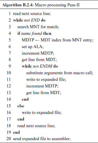
Macro Processing
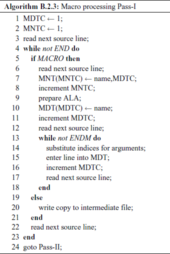
We shall assume that the macro processing is done independently of the assembler, as a preprocessing step. Also, we discuss only a simplified version, without nested macro calls or nested macro definitions. We have two passes – Pass-I will search for macro definitions and store them; Pass-II detect macro calls and expand them. The data structures used are:
MDT Macro Definition Table – stores the body of macro definitions.
MNT Macro Name Table – stores names of defined macros.
MDTC MDT counter – indicates the next available entry in MDT.
MNTC MNT counter – indicates the next available entry in MNT.
ALA Argument List Array – stores macro arguments and call arguments.
MDTP MDT pointer – indicates the next line of text during expansion.
The algorithms are given as Algorithms B.2.3 and B.2.4.
Macros and Subroutines
Seemingly, from the viewpoint of the programmer, macros provide the same kind of facilities as subroutines. Then how do they compare?
Macro: Complete macro body code gets substituted every time it is used, so increases the code length. As it is in-line code, save on the subroutine call and return instruction time and stack load overheads, and thus works fast.
Subroutine: Code is included only once in the program. Time and stack-space overheads for each call and return.
In summary, we can say that if the job can be done with a few instructions, say 5 to 10, then it may be advisable to implement it as a macro, otherwise it should be implemented as a subroutine.