
Chapter 4
Supply and Demand in
the Market for Goods
In the last chapter we referred to the way in which prices, acting as signals, direct production towards goods and services that people want to buy, and ration the available quantities among persons prepared to pay for them. Our present task is to examine more closely the working of supply, demand and price in the market place. In this chapter we will concentrate on the markets for goods or commodities. In the next, we will look at the working of the price mechanism in markets where factors of production are bought and sold.
We already know that the market price of a commodity depends upon demand and supply. Our next step is to examine more closely each of these. We shall proceed by considering demand and supply from the viewpoint of the individual consumer and supplier of goods. Then, by simply adding together demand by individuals, we can obtain what may be called total, or market, demand for a good. Similarly we can derive a notion of market supply, and finally put the two together to consider the formation of market price.
Demand
The demand that is of interest to economists is that which is related to the quantities of a commodity that individuals would be prepared to purchase. This is not the same thing as the quantities that they 'need', or would like to have. Needs and wants obviously lie behind purchases; but resources are limited, and our concern is only with actual market behaviour as revealed in effective demand backed by willingness to spend money.
We saw in the opening chapter that the amount of a commodity which people want to purchase is dependent upon many factors. Economists, however, find it convenient for expository purposes to concentrate upon one determinant at a time. The one in which prime interest resides is the price at which a commodity can be obtained.
Individual Demand
Let us take an example of a specific good, ice creams, and let us assume that a person's demand for this good, per period of time, depends upon such forces as the price of ice creams, the price of chocolates and other competing goods, the individual's income, his wealth, his tastes, the weather, and any other miscellaneous factors which may influence his desire to buy one. In the short run, we may reasonably suppose that all influences on demand, other than the price of an ice cream itself, do not change. We may then ignore the effect of all the other factors and concentrate on the demand for ice creams related only to their price.
This method of argument is commonly employed in economics when behaviour is known to depend on several factors. In such circumstances the analysis may be very complicated, and economists simplify the problem by a process of abstraction - analysing the influence of each determinant in turn, on the assumption that other determining factors do not change. The assumption is known by the name ceteris paribus, from the Latin 'other things remaining equal'. We shall use it several times in this book.
To make the point clearer, we can imagine a list of the quantities of ice creams that would be bought at various prices. Such a list is called a demand schedule. Table 4.1 shows demand schedules for two individuals whom we call Alan and Bill. The example is, of course, hypothetical, but it serves to illustrate the fundamental idea that demand has no exact meaning by itself, but only in relation to a particular price.
Table 4.1 Demand schedules for ice creams (hypothetical) (quantities demanded per week)

Demand schedules like those in Table 4.1 can also be presented graphically. If we measure price on the vertical axis and quantity demanded on the horizontal, we can draw a diagram for Alan and another for Bill as in Figures 4.1 (i) and (ii). DA is Alan's demand curve. It is constructed by plotting all the tabulated price-quantity combinations on the graph and joining them up. The curve shows, therefore,
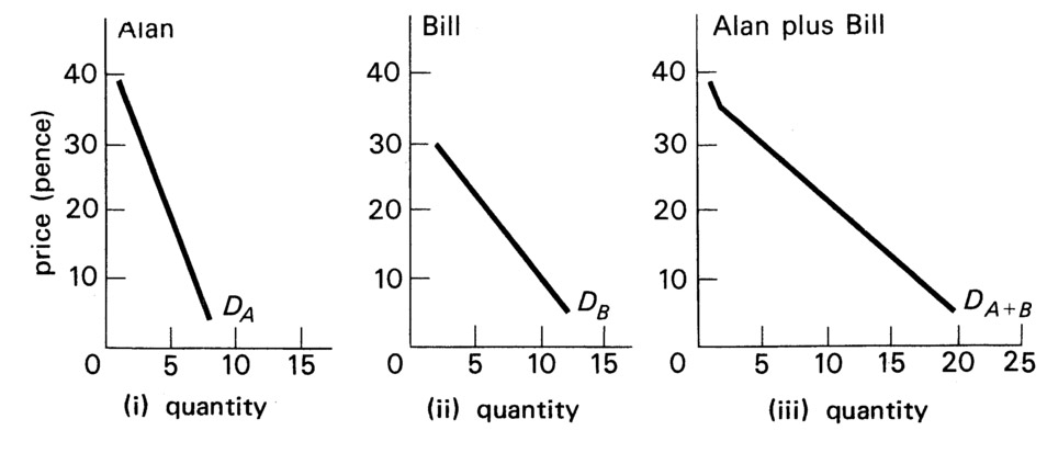
Figure 4.1 Demand curves for individuals and the market demand for ice creams per week.
the numbers of ice creams he would buy per week at every price between 5 pence and 40 pence. The same applies to Bill's demand curve in Figure 4.1 (ii).
We must now draw attention to an important characteristic of Alan's and Bill's demand curves. They are both downward sloping. This simply means that each of them demands more ice creams the lower the price. Why should this be so? The answer is related to the satisfaction they get from consuming ice creams. There is a widely accepted assumption in economics that applies generally to most commodities that the extra satisfaction (or utility as it is sometimes called) which one gets from consuming additional quantities of ice creams tends to fall the more one has of them.
The price one is prepared to pay for a good, it can be argued, depends on the satisfaction one gets from it. Moreover, the price one would pay for an extra unit of the good reflects the extra satisfaction obtained from consuming it. If this extra satisfaction, or marginal utility, falls with increasing quantities, then demand will be higher at low prices than at high. To put it another way, the price one would be prepared to pay for an additional unit falls as the quantity rises.
In our example, Alan is prepared to pay 40 pence for a single ice cream a week, but he will only be prepared to buy a second one if the price falls to 35 pence, a third if it falls to 30 pence, and so on. It would take a price of 5 pence to induce him to buy as many as eight.
This characteristic of consumer behaviour is known as the principle of diminishing marginal utility. Marginal utility is the difference in total utility derived from consuming an additional unit of a commodity. The principle can be stated differently. As consumption increases total utility increases, but at a decreasing rate. Whichever way the principle is put, it can explain the fact that Alan's and Bill's demand curves are downward sloping.
Market Demand
It remains to show how to derive the market demand curve from the demand curves of individuals. We start by returning to the demand schedules in Table 4.1. If, now, we add together the demand schedules for Alan and Bill, and assume that they comprise the total number of persons who buy ice creams, we have, in the last column of Table 4.1, the total market demand schedule. Similarly, in Figure 4.1 (iii) we can 'add' the demand curves for the two persons. This is done by constructing the line DA+B in Figure 4.1 (iii) by adding horizontally the quantities demanded at each price. Thus, at 40 pence and 35 pence each, only Alan buys ice creams, so the market demand curve is exactly the same as Alan's. At a price of 30 pence, however, Alan buys three ice creams, but Bill also buys two, so the market demand is for five ice creams at that price, and so on. It should be noted, too, that the market demand curve, like those of Alan and Bill is downward sloping. This is not surprising because it is constructed from two demand curves, those of Alan and Bill, which are themselves downward sloping. There is, however, an additional reason. It is simply that falls in price not only induce increasing demand by existing consumers, they also attract new consumers into the market — people who do not consider purchases at higher prices. Referring back to Table 4.1, we can see that Alan is the only consumer as long as the price is 35 or 40 pence. At a price of 30 pence, however, Bill enters the market. The additional consumption of three ice creams is partly due to Alan buying one more, but also to the fact that Bill starts off by buying two ice creams.
The explanation given in the previous paragraph suggests that market demand curves are even more likely to slope downwards than the demand curves of individual consumers. This characteristic of demand curves is believed to have widespread, if not universal, application to demand curves in general.
There is a final feature of market demand curves that must be mentioned. It is that they may be affected by certain factors other than those determining the demand curves for individual consumers. These are all by way of being usually long-run considerations. The most commonly included are the size of the population of a country and the distribution of income within it. The latter is not only a question of size distribution between rich and poor, but also distribution of any kind which might affect total demand. For example, a redistribution of income from older to younger people could easily raise the demand for LP albums and lower the demand for wheeled shopping baskets. In the short run, matters like the size of the population and the distribution of income are included in the ceteris paribus assumptions described earlier, that is, they do not change during the period being analysed.
Income and substitution effects of price changes
We may gain further insight into the reasons why demand curves tend to slope downwards by considering that there are really two distinct aspects of a price fall that lead to a change in the quantity purchased. These are known as the substitution effect and the income effect. The nature of the substitution effect is obvious. When the price of any good falls while the prices of all other goods remain unchanged, there is a natural tendency for people to buy it instead of other goods — that is, to substitute it for similar or competing commodities. But there is an additional reason why demand may change when price falls. Among our ceteris paribus assumptions, it may be recalled, is that of a constant level of the consumer's income. But when an individual has a fixed money income and the price of one of the goods he buys falls, this effectively raises his real income, that is, its purchasing power increases. A rise in income means that a person has more to spend on all goods. It is likely that he will use some of this extra to buy more of the commodity whose price has fallen.
Earlier (in Chapter 1, page 7) we distinguished between normal and 'inferior' goods. Those the consumption of which rises (or falls) as income rises (or falls) are called normal. Those which are bought in smaller quantities as income rises are known as inferior. Provided that the good whose price falls is not an inferior good, the income effect of the price change, as well as the substitution effect, will tend to increase the quantity demanded.
Although most demand curves, as argued above, slope downwards, the steepness of the slope varies from one commodity to another. To put the matter differently, when the price of a good changes, the extent to which this leads to a change in demand is not the same for all goods.
The reasons for this are related, to a considerable extent, to what we have called the substitution effect. The more and better substitutes that a good has, the more one may expect demand to increase for a fall in price (or to decrease for a rise in price). In part, this may merely reflect how closely a commodity is defined. 'Kodak 35 mm cameras' have more substitutes than '35 mm cameras', which in turn have more substitutes than 'cameras'. But it is also true that there are more good substitutes for, say, tomato sauce, than for, say, salt.
The income effect is relevant to the extent to which demand for a good responds to price changes. If the good is an inferior one, the income effect will dampen the substitution effect. For a normal good, in contrast, the rise in real income tends to reinforce the increase in demand following a price fall. For any commodity, however, one can add that the more important the item in the consumer's budget, the stronger the income effect is likely to be. A good such as ice creams in our earlier example obviously absorbs so small a part of a consumer's budget that a change in price of a few pence can hardly have a significant effect on his real income. In contrast, a fall or rise in the price of houses, for instance, may very well be expected to make a consumer significantly better or worse off by changing the effective purchasing power of a fixed money income.
A matter relevant to the relationship between price and quantity demanded is the number of uses to which a good may be put. In general, the greater the number of uses, the larger the change in demand to be expected, for the greater is the scope for extending demand after a price fall (and vice versa). Tea, for example, has fewer uses than eggs, so that a fall in the price of tea may be likely to cause a relatively smaller rise in demand than a fall in the price of eggs.
Finally, it should be mentioned that the responsiveness of demand to price changes tends to be larger the longer the time period under consideration. This is true for both rises and falls in price, and reflects the fact that some people often take quite a while even to hear about price changes. Very few people are also so flexible that they adjust their habits instantly the price of a good rises or falls.
Elasticity of Demand
Economists have a special way of measuring the responsiveness of demand to changes in price - they call it elasticity. Formally, the elasticity of demand is a fraction (or ratio) — the proportionate change in quantity demanded divided by the proportionate change in price. For a commodity which has many substitutes, and whose demand responds easily to price changes, the fraction is larger than 1, and demand is said to be elastic. If a 1 per cent price fall causes a 2 per cent rise in quantity, for example, a good would be in elastic demand.1
In contrast, a good which has few substitutes, and for which the demand responds weakly to a price change, would have an elasticity of demand of less than 1, and demand would be said to be inelastic, A 5 per cent price fall leading only to a 1 per cent increase in quantity would be an example of this kind of good.
Between the two cases mentioned we may discern a third, benchmark, category, comprising goods for which the demand responds to a given percentage price change by changing in quantity by exactly the same percentage. If demand falls by 1 per cent, the elasticity of demand is said to be equal to unity. It is not hard to see that, for such goods, total expenditure on the commodity is identical at all prices. But we may observe that for goods for which the demand is elastic, total expenditure increases as price falls (since demand expands relatively more than price falls). Conversely, for goods for which the demand is inelastic, total expenditure increases as price rises (since demand does not fall off relatively as much as price rises).
Before leaving the explanation of the term elasticity of demand, it should be mentioned that the concept of elasticity, measuring the responsiveness of one factor to a change in another, is not confined to demand, but is widely used in economics. For example, the income elasticity of demand measures the responsiveness of demand to changes in income, and there are many others.
Changes in Demand
We argued earlier that it was often reasonable to make ceteris paribus assumptions about factors such as income, tastes, and so on, which affect demand. These assumptions were necessary in order that a demand curve might be derived at all. But it does not follow that we must always retain the assumptions in our analysis of market behaviour. Suppose in fact, that a change in a ceteris paribus assumption occurs. We sometimes refer to such a change as one in the conditions of demand. All we need to do is to draw a new demand curve. An example may help to make the matter clear. Imagine something happening, such as the discovery that ice cream stops baldness, which makes people decide they want to buy more ice cream. We could interpret this change as a shift to the right of the demand curve DD to D'D' in Figure 4.2, implying that at every price the quantity demanded is greater than it was before. A fall in income, in contrast, might shift the demand curve back again to DD, as might an appropriate change in any one of the determinants of demand other than price.
It must be emphasised that changes in the price of a good itself do not shift the demand curve. We read the effects of price changes by moving along the curve. It is important to avoid the common error of confusing these price changes with changes in the ceteris paribus assumptions. These last shift the whole curve if they vary. The extent and manner in which they alter the position of the demand curve depends upon the nature of the good in question. A fall in the price of
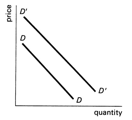
Figure 4.2 An increase in demand.
a substitute for a good tends to shift the demand curve downwards — less being bought at every price when there is a cheaper substitute available. But there are also goods which are complementary to each other, which tend to be demanded together, and which cause opposite kinds of shifts in demand curves. Tennis racquets and tennis balls are, for example, complements. A fall in the price of racquets tends to shift the demand curve for tennis balls upwards, more balls being demanded as soon as people buy more (cheaper) racquets.
Supply
We must now shift our attention from demand to examine more closely the determinants of the supply of a commodity. Supply, like demand, depends on many factors. The principal ones are the costs of production, the kind of market in which business operates, and the objectives or goals at which the owners of a business enterprise are aiming.
As we explained in Chapter 2, it is usual in economics to assume, as a first approximation, that firms are in business primarily to maximise profits. Although this is clearly not true in every case, we can safely adopt the assumption here in order to derive certain elementary conclusions about market behaviour. It may need qualification later, when alternative goals, such as maximum sales or growth of the business, are substituted for it. We assume, too, that the market is a competitive one comprising a large number of small firms. We shall return later in this chapter to consider the implications of this assumption.
Supply by an Individual Firm
Our concern at the moment is to relate quantities supplied to price. We wish to derive a market supply schedule for a commodity in which the amounts offered for sale are related to a range of prices. Such a supply schedule must be built up from the schedules of amounts supplied by individual firms, including both existing businesses and firms which might enter production if price were high enough.
Consider again the hypothetical case of the supply of ice creams. Suppose that there were only two firms in the market. Their supply schedules might be those shown in Table 4.2. (The numbers are kept deliberately if unrealistically small.) As in the case of demand, we can plot the supply curves on graph paper as in Figures 4.3 (i) and 4.3 (ii).
In contrast to the demand curves of Figure 4.1, the supply curves of both firms slope upwards. This feature of the supply curve is related to the cost structure of firms. If a firm is to be induced to offer additional
Table 4.2 Supply schedules for ice creams {hypothetical) (quantities supplied per week)

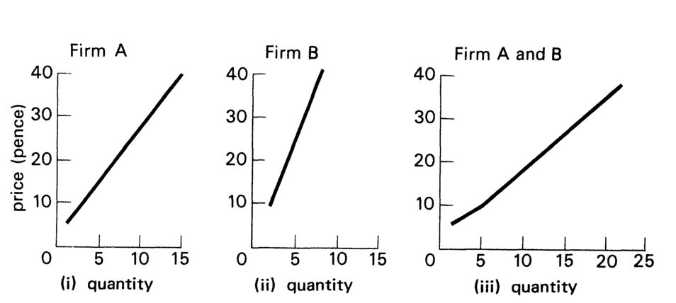
Figure 4.3 Supply curves for individual firms and the market supply of ice creams per week.
units of a commodity for sale, it is obvious that the price at which it is able to sell them must cover their costs of production.2 An upward sloping supply curve implies that the higher the price the larger the quantities that would be offered for sale. The justification for such an upward slope, then, may be that costs rise, at the margin, as output increases. For this reason a rise in price may be seen as necessary in order to cover the addition to total costs occasioned by the higher output.
The changes in total costs attributable to changed output are known as marginal costs. We shall assume here that marginal costs rise as output increases, so that we may examine the determination of market price in such a situation. We must realise, however, that if costs do not increase then the supply curve need not be upward sloping. Some of the implications of dropping this assumption may be quite readily appreciated, but the reader is warned that certain others must await more advanced work in economics.3
Market Supply
The derivation of the market supply curve from the supply curves of firms A and B is straightforward and basically similar to the method of deriving the market demand curve of Figure 4.1 (iii). At a price of 5 pence, firm A offers one for sale, firm B none at all, so market supply is one. At a price of 10 pence firm A offers three, firm B two, market supply is five, and so on.
Finally it should be noticed that the market supply curve like those of firms A and B slopes upwards and in the opposite direction, therefore, to the market demand curve. The reasoning here is basically similar to the case of demand. There are again two explanations. First, a rise in price calls forth a larger quantity from existing suppliers and, secondly, it attracts other firms into the industry.
Elasticity of Supply
It was mentioned earlier that the concept of elasticity had several uses in economics other than in relation to demand. One such is the elasticity of supply — a measure of the responsiveness of supply to changes in the price of a commodity.
Elasticity of supply is defined as a fraction (or ratio), the proportionate change in quantity supplied divided by the proportionate change in price that brought it about. Goods for which supply responds readily to price changes are said to be in elastic supply. The numerical value of the fraction is greater than one, implying that a price rise (or fall) induces a more than proportionate rise (or fall) in the quantity offered for sale. Conversely, goods the supply of which responds only weakly to price changes are said to be in inelastic supply and the numerical value of the fraction is less than one. There is also a benchmark case of unitary elasticity of supply, where the fraction has a value of exactly one and the proportionate changes in quantity supplied and in price are the same.
When we come to identify the factors responsible for deciding whether elasticity of supply is likely to be great or small for a particular good, the question of the availability of substitutes is of great importance, as it was in the case of demand. Substitutes in supply, however, have a rather different significance. In order for supply to be readily responsive to changes in price there must be ready alternate occupations for factors of production. In other words, there must be goods to or from which production can readily be switched.
Compare, for instance, the supply ot plastic toy cars with that of potatoes. In the former case, one might reasonably expect that it was relatively easy for a firm to switch labour and other resources from producing plastic cars to any of an obviously wide range of other plastic toys. The responsiveness of supply to changes in the price of toy cars would, then, tend to be relatively greater than that to a change in the price of potatoes. Once potatoes are planted, there is no scope at all in the short run for a farmer to switch to another crop. This example also brings out the point that elasticity of supply, similarly again to that of demand, tends to be greater the longer the time allowed for adjustments to take place.
Changes in Supply
Supply curves, like demand curves, are drawn up on ceteris paribus assumptions; in this case to allow the relationship between price and quantity supplied to be isolated. Foremost among the factors which are assumed to remain unchanged over a period are costs of production behind which lie such matters as the state of technology and the prices of the factors of production used by firms. This assumption does not mean that costs do not vary with output, but that the relationship between costs and output does not change over time. If any change of this kind occurs it is often referred to as a change in the conditions of supply. We can deal with it in a similar way to that in which we dealt with shifts in demand. We can move the entire supply curve.
Suppose, for example, a new invention makes possible a lowering of costs of ice cream production. We can interpret this as a downward movement of the entire supply curve as from SS to S'S' in Figure 4.4, implying that a larger quantity would now be supplied at every price.
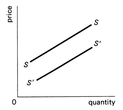
Figure 4.4 An increase in supply.
Market Equilibrium
We have now derived independent relationships between demand and price, and between supply and price. Let us put together the market demand and supply schedules and curves which we invented for ice
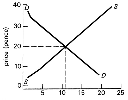
Figure 4.5 Equilibrium market price, where supply equals demand.
Table 4.3 Quantities of ice creams demanded and supplied per week

creams in Table 4.3 and Figure 4.5. Remember that DD portrays the quantities that consumers wish to buy at various prices, while SS shows the quantities that suppliers wish to offer for sale at the same set of prices.
It can be seen that only when the market price is 20 pence are supply and demand the same — or, to put it another way, that the market is cleared and there are no disappointed consumers or suppliers. In such a situation, market price is said to be at an equilibrium level.
The meaning and nature of equilibrium can best be understood by examining the likely consequences of any other price obtaining in the market. Suppose, for example, market price were below equilibrium, say, at 10 pence, consumers would want to buy seventeen ice creams, but only five would be offered for sale. The resulting excess of demand over supply would tend to force the price up towards equilibrium, as consumers competed with each other for the limited supply. Conversely, at a price in the market above the equilibrium, there would be the opposite situation, an excess of supply over demand. At 35 pence for an ice cream for instance, market demand is only two, whereas twenty would be offered for sale. Market forces on the supply side would now tend to push price downwards, as sellers competed with each other to dispose of their stocks. The market is in equilibrium only where the supply and demand curves intersect, at a price of 20 pence, and with eleven ice creams being bought and sold. Only then is there neither excess demand nor excess supply. The market is cleared and there are no market forces acting on the price to change it.
A word must be added about the nature of market equilibrium, which is sometimes thought to carry with it overtones of desirability. We must emphasise that its meaning is quite technical. The statement that a market is in equilibrium means no more than what it says - that is, that price is such that the quantity suppliers want to sell is equal to the quantity consumers want to buy. There is nothing necessarily good about it.
It is true that we argued earlier in this book that a market system using the price mechanism might achieve an allocation of resources which could be judged as efficient from the viewpoint of consumers. But this statement is highly conditional. It carries the conclusion that such an allocation will in fact be ideal only if certain conditions relating to the market and the economy obtain. These preconditions were listed towards the end of the last chapter, where it was made clear that the market would fail if one or more was not present. We shall return to deal more fully with them later.
Applications of Supply and Demand Analysis
The framework for the analysis of market price just described has an almost unlimited number of uses in economics. A few illustrations may be given.
A Change in Tastes
Suppose that a market is in equilibrium and there is a change of tastes. Say, for instance, that people start to like ice cream less than they did before.
Readers should be on their guard here against one of the most common mistakes made by students commencing the study of economics, when they confuse movements along with shifts of a supply or demand curve. Remember always that a demand curve, or a supply curve, is drawn on ceteris paribus assumptions to show the relationship between price and quantity demanded or supplied. If there is a change in one of these assumptions, this means that there is a change in the conditions of demand or supply, and the entire curve shifts as the relationship between price and quantity alters at every price. In our example here, the change in tastes is just such a change in the conditions of demand, and its effect is to shift the whole demand curve downwards to the left. Since there is, however, no change in the conditions of supply, the lower quantity supplied in the new equilibrium situation results only from the fall in price. The supply curve itself does not shift.
We can represent the change in the conditions of demand, as in Figure 4.6 (i), as a downward shift of the demand curve for ice creams from DD to D D'. The effect is that the market tends towards a new equilibrium (E') at the intersection of SS and D'D', where both price and quantity have been reduced, from OP to OP' and from OQ to OQ respectively.
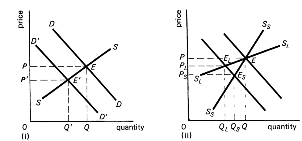
Figure 4.6 Fall in demand in the short run and long run.
Short-run and long-run effects
We can take the analysis one stage further if we remember that supply tends to be more responsive to changes in price the longer the period of time we allow for adjustment. In Figure 4.6 (ii) there are two supply curves going through the original equilibrium point (e). SsSs is the short period supply curve. SLSL is the curve for the longer period. The difference between them is simply that the long-run supply curve shows a higher degree of responsiveness of quantity to a change from the equilibrium price, that is, demand is at that price more elastic, than the short-run curve. It may be seen too that in the long run a fall in demand tends to have a less depressive effect on price, but a larger effect on sales, than in the short run. Initially, the quantity supplied falls only from OQ to OQS, causing price to fall from OP to OPS. But as supply falls further in the long run to OQL, market price partly recovers to OPL.
The influence of time on the demand side can be similarly illustrated. The reader might try to draw for himself a pair of diagrams showing how a decrease in supply, following a rise in costs, can raise price more in the short run than in the long run.
From the analysis in this section, we can derive a general conclusion. The more elastic supply and/or demand, the more a change in either of them is likely to lead to changes in quantities bought and sold, and the less to changes in price. Consider, for example, the two goods in Figure 4.7. In part (i) of the diagram, both the demand for and the supply of pencil sharpeners are assumed to be very responsive to changes from the equilibrium price. The rise in demand depicted has a relatively smaller effect on price than on the quantity demanded and supplied.
In Figure 4.7 (ii), in contrast, the supply of and demand for cocoa are both assumed to be relatively unresponsive to price changes. In this case, the rise in demand is seen to be reflected in a larger change in market price and a smaller change in quantity.
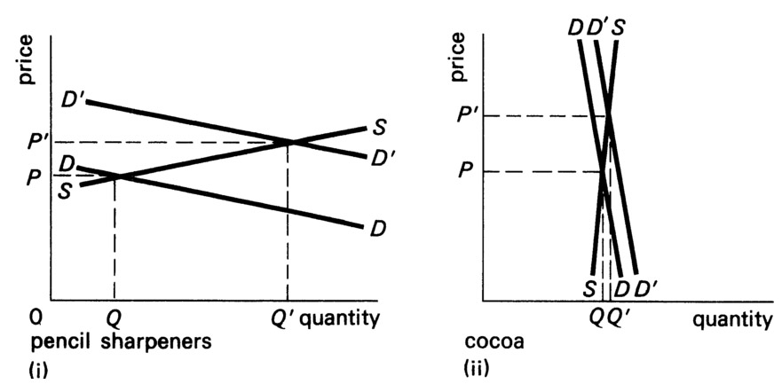
Figure 4.7 Rise in demand. Elastic and inelastic supply and demand.
Agricultural Markets
It is no accident that the commodity taken to illustrate the last paragraph and Figure 4.7 (ii) is an agricultural product, cocoa. Both supply and demand tend to be inelastic with respect to price for many agricultural products. Supply is typically inelastic, particularly in the short run. Once a crop is planted, the size of the harvest is likely to be mainly determined by such factors as the weather and the incidence of disease. Even in the longer run the supply of some agricultural products may still be relatively fixed, for example, in the case of orchard crops, where years can elapse between planting and fruit gathering. Price inelasticity tends to be low on the demand side as well. This is true not only for foodstuffs, but also for raw materials, like rubber and cotton. Quantities demanded typically rise and fall more with changes in consumers' incomes than with changes in price.
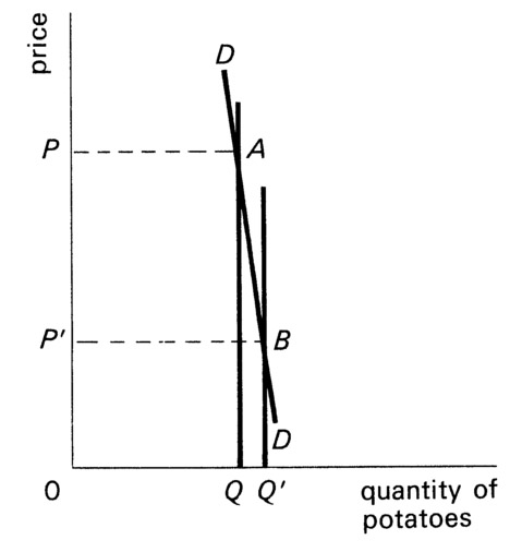
Figure 4.8 A change in supply, under conditions of inelastic demand, changes total revenue.
The implications of inelastic supply and demand in a market are illustrated in Figure 4.8 for an agricultural product, such as potatoes. We assume that good harvest-time weather increases the quantity available for sale from OQ to OQ'. The consequences of the larger crop can be seen from the diagram to be serious for potato farmers. Not only is there a substantial fall in price from OP to OP, but total revenue of the farmers falls with the larger crop. Price multiplied by quantity, OP' times OQ', is less than OP times OQ. (Or the rectangle OP'BQ' is smaller than OPAQ.) This happens because demand is inelastic, so that the proportionate rise in quantity sold is less than the proportionate fall in price.
The kind of situation illustrated in the diagram typifies market behaviour for many agricultural products. It is not surprising that, in addition to agriculture being subject to relatively large price fluctuations as crop size varies, farmers' incomes tend also to rise and fall from year to year. Farmers are inclined to be relatively well off when harvests are small, and badly off when they are large. For this reason it is common to find that governments in most countries tend to intervene in agricultural markets with various kinds of schemes to lessen the impact on farmers of short-run market forces, and to stabilise to some extent farm incomes and prices.
Taxation
A last example of the application of supply and demand analysis is the case of a specific tax on a commodity. Suppose the government decides
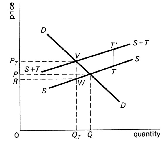
Figure 4.9 A specific tax; effects on price, quantity and government revenue.
to impose a tax of a penny on a box of matches. What are the consequences for (a) market price and (b) sales? And (c) how much revenue will the government obtain?
The answers to these questions are suggested by looking at Figure 4.9. SS and DD are the original supply and demand curves. Market equilibrium is OQ sales at price OP. A tax equal to TT' (representing 1p per box of matches) is now imposed. Assume that sellers are given the responsibility of paying this tax to the government. They will no longer be willing to supply the same quantities at the same range of prices as they did before. We can imagine them adding the tax to each price at which they would be willing to supply a given quantity. We can depict this by drawing a new supply curve (S + T) parallel to SS, such that the vertical distance between them is equal to the tax itself {TT').
Note that we cannot assume that market price also rises by the full amount of the tax. In our diagram it certainly does not do so. When the new equilibrium is reached, market price will be OPT and sales OQt. Consumers' total expenditure is OPT VQT, which is what suppliers receive. Out of this total, sellers must pay VW (= TT')) per unit to the government, so that total tax revenue to the state amounts to PT VWR. Market price, however, has risen only b JPPT, which is less than the full amount of the tax TPt.)- We could explain this phenomenon by suggesting that as market price rose when the tax was imposed, demand started to fall off, and in order to limit the extent of the fall in sales, suppliers effectively absorbed part of the tax themselves.
We cannot investigate the full implications of the analysis in this volume, but enough has been said to show that the effect of a tax on market price may be related to the elasticity of demand and supply of a particular good. (Using the argument of Figure 4.7, can you work out what kind of supply and/or demand curves would lead to price rising more or less than in Figure 4.9? Hint: try (1) changing the slope of the demand curve while retaining the supply curve and then (2) keeping the same demand curve and changing both SS and S + T.)
It can be added that the analysis of this section on taxes is equally applicable to subsidies, which can be viewed as no more than negative taxes. In the example of Figure 4.9, we could start with the curve S + T as the original supply curve and relabel the S curve as S — S with TT' being the subsidy received per unit of output by producers, enabling them to offer their goods to consumers at a lower price for each quantity they offer for sale. Market price would then fall from OPT to the new equilibrium OP (less than by the full subsidy) and PT VWR would now be interpreted as the cost of the subsidy to the government.
Economic Welfare
We have now dealt with a number of situations where the action of the price mechanism leads to an equilibrium situation where supply and demand are equal and the market is exactly cleared. When we first encountered the notion of equilibrium we were at some pains to point out that its meaning was technical and did not carry with it the implication that it was necessarily desirable.
We must return to consider this matter further. Our choice of words was careful and deliberate. Although there is nothing necessarily desirable about resource allocation brought about by the market, there is a case to be made that in certain circumstances such an allocation might be regarded as in a sense ideal or, to use economists' jargon, 'optimal'.
Some of the advantages of a market system were briefly described in Chapter 3. We are, however, now in a position to understand better the argument why the price mechanism can in certain conditions be regarded as an efficient means of allocating resources. Let us reconsider the case for laissez-faire, as we have earlier described it, that economic welfare is maximised in a market system.
The Case for Laissez-Faire
Laissez-faire implies no interference with the market because the price mechanism will allocate resources optimally if left alone. The case for such a policy is not particularly easy to understand and it is most important to follow carefully each step in the argument. It can be put like this. In equilibrium, market price measures two things — the marginal cost of producing a good and the marginal utility (or satisfaction) obtained by consuming it. Price measures marginal cost because sellers offer an extra good for sale only if it yields a revenue which covers the cost of producing it. Price measures marginal utility because (if we assume that consumers try to maximise their satisfaction in disposing of their incomes) buyers purchase an extra good only if it yields enough utility to make the expenditure on it worthwhile. Producers go on offering more of a good for sale if price is greater than marginal cost; consumers continue buying more of a good if price is less than marginal utility. Hence, when price is at an equilibrium level, and is the same for all producers and consumers, we can draw the inference that marginal utility is equal to marginal cost.
We may usefully recall, now, our discussion of the true nature of costs in economics. The opportunity cost of producing a good is the sacrifice made in not producing another good. So the equality of marginal cost and marginal utility at equilibrium means that the benefit derived by consumers from purchasing an extra unit of a good is equal to its cost as measured by the opportunity foregone of having more of another good in its place.
If marginal cost is not equal to marginal utility, satisfaction can clearly be increased by switching resources between products. If there is a commodity where marginal utility is greater than marginal cost, it is worth producing more of it because the sacrifice of other goods given up is less than the marginal increase in satisfaction from having more of it. The opposite is true if marginal utility is less than marginal cost. Hence, if marginal cost is brought into equality with marginal utility through the operation of market price, satisfaction of the community cannot be increased by producing more or less of the good. Moreover, if marginal cost is equal to marginal utility in the market for every single good and service, it follows that the distribution of resources is, in a sense, optimal.
It must be emphasised that the case for laissez-faire is an abstract one. Its acceptability, in whole or in part, depends on the extent to which it is relevant to the world in which we live. In the last chapter (pages 52-3) we listed six conditions which, if applicable, would mean that a market system would be likely to allocate resources efficiently. They will all be discussed at greater length when we deal with economic policy in Chapter 10. However, we are now in a position to explain why two of them are important for the case for laissez-faire.
Income Distribution and Market Allocations
One reason for questioning whether the allocation of resources that results from the free interplay of the forces of supply and demand is efficient arises from issues of justice and equity in the distribution of income in a country. This is, at least partly, a political matter. However, our immediate task is the economic one of showing the implications of income distribution for resource allocation. Let us suppose that we ignore the social issues of equity and accept the distribution of income as given.
The price mechanism will then work in the manner described in the last section to allocate resources so that marginal utility is equal to marginal cost in each and every market throughout the economy. Let us further assume that the initial distribution of income was very unequal. We might then conclude that the market will succeed in securing the production of a fair amount of champagne, yachts, Rolls-Royce cars and luxury hotels.
Suppose we now imagine that it is considered socially desirable to redistribute income more equally by taking from the rich and giving to the poor. It is clear that there will be a shift in demand away from goods of the kinds mentioned above bought by high-income groups. Market forces of supply and demand will still operate to shift resources until marginal cost is equal everywhere to marginal utility. But the collection of goods and services now produced is likely to be quite different. What can we say now? Both allocations result from the free working of the price mechanism, so it is difficult to say that one or other is the 'best'. We can only choose between them if we have some reason for preferring the more or the less equal income distribution, within the framework of which the market system did its work.
The reasoning of the previous paragraph requires us to reassess the implications for economic welfare of equilibrium price and output achieved in a market system. If we are prepared to accept the distribution of income as being in a sense desirable, then we can have no doubts, on this count, about accepting the allocation of resources brought about by the free working of the price mechanism as being optimal. But if we recognise that we, as economists, have no special authority to make this kind of value judgement, we must also be careful to avoid concluding also that the market works well. We can only make the much more limited conclusion about the nature of equilibrium — namely, that it is the state of affairs towards which economic forces of supply and demand will tend in the market place. The equilibrium quantity of ice creams, or of anything else, is that quantity which, if produced, leaves no unsatisfied buyers or sellers. But we must remember that supply and demand are really no more than 'catch-alls', behind which lie all the social forces which may influence them. The question of what is the best distribution of income is not at all easy to answer. Economic as well as social considerations are involved and, in so far as inequality might provide incentives for maximising output, they must be taken into account as well as ideas of social justice. We shall return to discuss the implications of these matters for economic policy in Chapter 10.
Competition and Market Allocations
A second reason for questioning the efficiency of a market system relates not so much to the social framework as to the nature of the market itself. In order to appreciate the significance of competition for resource allocation in market economies, we shall have to engage in one more piece of analysis.
Most of this chapter has been based on an assumption that markets are competitive. However, there are degrees of competition. Economists classify markets according to whether competition is said to be 'perfect' or 'imperfect'.
(1) Perfect competition
At one extreme there is a highly competitive state of affairs, wherein a large number of small producers each sells a commodity which is no different from that of any other producer and there is complete freedom of entry for firms into the industry. In such circumstances no single seller can by himself influence price in the market by withholding supplies; he is too small. He is a price-taker and the market is termed perfectly competitive. And, although it may be rare enough in the real world, it provides a useful reference base against which other market situations may be compared.
(2) Imperfect competition
At the other extreme from perfect competition is the case of the single seller or monopolist dominating a market. Monopoly is one of a number of market forms classed under the heading of imperfect competition (though the terms perfect and imperfect relate only to the intensity of competition, not to their desirability or undesirability). Other forms include oligopoly (from the Greek meaning few sellers).
Sources of monopoly power. Firms in imperfect competition are generally in stronger positions than those where competitive forces are intense. Their strength is derived in divers ways. Such firms may control the supply of a raw material. They may hold a patent giving them the sole legal right to some manufacturing process. Their strength may stem from being the only shop selling a certain range of goods in a particular locality. They may market a product which is differentiated from others and for which consumers feel a special loyalty. They may enjoy the benefits of large-scale production economies, so that their costs are too low for other firms to compete with them.
Firms enjoying a degree of monopoly power are not, of course, free to ignore the market entirely. Their actions are constrained to a varying extent by consumer demand and by actions of other firms. The point is only that the competitive forces to which they are subject tend to be weaker. However, firms which do possess some control over the market have one thing in common, wheresoever they draw their strength. They enjoy the opportunity to earn higher profits than would otherwise be the case.
Under conditions of perfect competition, as we have seen, the presence of profit-maximising businesses leads to an inflow of firms into industries making above-average profits. But in imperfectly competitive situations, the sources of market power, whereby firms derive their strength, act as barriers to the entry of other firms. As long as the barriers persist, for example until patents run out, other firms acquire know-how, and so on, those businesses already in the industry are protected from the full blast of competition.
Single-firm monopoly behaviour. The analysis of a firm's behaviour under conditions of imperfect competition are complex and cannot be described fully here. However, one important characteristic must be discussed.
Compare the position of a single-firm monopolist with that of a firm in perfect competition. Assume, too, that both are trying to maximise their profits. The perfectly competitive firm is too small to exert any perceptible influence on the market by changing the quantities he offers for sale. He can sell as much or as little as he likes without affecting market price. In contrast, the monopolist is a price-maker, by definition; he is so large that when he alters his output market price is affected. He can only succeed in selling additional quantities if he does lower price. Moreover, since only one price can normally exist in a market for the same commodity, when the monopolist lowers price to sell another unit, he must lower it on all the units that he sells.
The implications of this feature on the output policy of a firm can be understood by reconsidering what is meant by our earlier statement that a seller offers goods for sale up to the point where the price he gets for them covers his marginal costs. This is true for the firm under perfect competition, because the price he receives is only another way of saying the increase in revenue he obtains from selling an additional unit. Economists call the change in receipts following an increase in the quantity sold marginal revenue. It is defined as the total revenue from the sale of n units, minus the total revenue from the sale of (n — 1) units.
For a small firm in perfect competition, marginal revenue is equal to price. But for a monopolist, the sale of an extra unit of a good is only
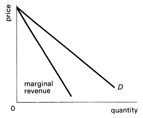
Figure 4.10 Marginal revenue under imperfect competition.
attainable by reducing price, not only for the additional unit, but for all the goods sold. In other words, marginal revenue is always less than price, and we can draw a marginal revenue curve which lies below the demand curve, as in Figure 4.10.
An example may help to make the matter clear. Suppose a large firm can sell 60 units at a price of £1.00 each, but in order to sell 61 units the price must be lowered to 99 pence. The increase in total revenue which the monopolist receives from the 61st sale is not 99 pence but 39 pence. He adds 99 pence by selling one more unit at 99 pence but loses 1 penny on each of the 60 previous sales. In other words, his marginal revenue of 39 pence is the total revenue from 61 units (61 x 99 pence) minus the total revenue from 60 units (60 x 100 pence).
Whereas we said earlier that a firm produces up to the point where marginal cost is equal to price, we now know this really meant: up to the point where the extra cost was just covered by the extra receipts — i.e. where marginal cost equals marginal revenue. Although price and marginal revenue are the same for a firm in perfect competition, the monopolist, as we have seen, finds that marginal revenue is less than price. Hence, he maximises profits by producing less than the competitive output. In Figure 4.11 the equilibrium position is where the monopolist produces an output of OA that is, where the marginal cost curve cuts the marginal revenue curve. Competitive output, where marginal cost equals marginal utility, would be OB.
Monopoly and market efficiency. After this brief excursion into the analysis of monopoly equilibrium, we must return to the question with which we started. How does the existence of imperfect competition affect the conclusion that the price mechanism allocates resources in an optimal manner? The particular feature of the monopolist's behaviour in Figure 4.11 that is relevant is that the profit-maximising output OA

Figure 4.11 Monopoly
sells in the market at the price OP, which is greater than the marginal cost OR. If we recall that price is a measure of marginal utility of a good to consumers, we must draw the implication that monopoly equilibrium tends to result in marginal utility being greater than marginal cost, and that an increase in output would add more to consumer satisfaction than to costs. Since costs in economics are opportunity costs, this means that, prima facie, resources used in the output of a good produced in such circumstances involve, at the margin, a sacrifice of other goods of less value than the satisfaction that they provide to consumers.
We may conclude that the presence of monopolistic elements in a market tends to lead to less production than would occur under competition; and that (by the standards which we applied for judging the efficiency of the price mechanism for allocating resources) output is, ceteris paribus, less than optimal. Since we know that the world is characterised by markets in which competition is to varying degrees less than perfect, we have good reason to view with caution the argument for non-interference in the working of the market system. We must be equally careful, however, not to jump to the conclusion that the price mechanism should necessarily be jettisoned, though it clearly cannot be relied on to work in a completely free fashion to secure an optimal allocation of resources.
Even the case against monopoly outlined above, which rests on underproduction, is not complete. For one thing, there are reasons for believing that the economies of large-scale production, mentioned earlier as sources of monopoly power, really do mean that costs may be lower for single firms than for several. In terms of Figure 4.11, this means that the curve labelled MC would be downward sloping. Breaking up such 'natural monopolies', as they are called, in order to promote competition would only involve higher costs of production on average. So it becomes a matter of judgement to decide whether or not, on balance, the presence of monopoly involves less than optimal output.
To complicate matters further, it should be added that monopolies may be inefficient in another sense. Their costs of production may be higher than they need be. They are not under the same pressure to minimise costs as if they were in more competitive situations. Such higher production costs are said to be the result of 'X-inefficiency'.
We may conclude that the question of judging the efficiency of market systems is a complex one. We shall reconsider it in Chapter 10 when we deal with economic policy. Meanwhile we turn to a consideration of the way in which supply and demand work in markets for factors of production.
Notes: Chapter 4
1 The most common formula for the calculation of elasticity of demand (known by the symbol ŋd) is: change in quantity change in price  quantity price So if a fall in price from £100 to £99 brings about a rise in quantity demanded from 200 to 204:
Readers are advised to consult more advanced texts about alternative ways of interpreting the formula.
2 Costs here are defined to include an element of profit, which economists call 'normal profit', defined as the minimum necessary to persuade a firm to produce in its existing market. Normal profits are related to the opportunity cost of capital - the amount that could be earned by switching resources to an alternative industry.
3 There are even difficulties in drawing a supply curve at all.