Chapter 11
The Methods of Economics:
Tools and Techniques

The reader who has reached this last chapter will, hopefully, have found out for himself the answers to the questions what do economists do and how do they go about their job. This is the best way to learn. But the student may find it useful to have the main ideas of the methods of economics now brought together.

The Social Sciences

Economics belongs to the group of subjects known as the social sciences. The term includes sociology, social psychology and political science, and the subjects share two important characteristics. They are 'social' and they are 'scientific'.

(1) ‘Social’

The subject-matter of the social sciences is human behaviour, past, present and future. There is no point in trying to define the boundaries of each subject. They overlap and cannot be defined precisely. It was once fashionable to consider the merits of alternative definitions of economics in textbooks. But the only faultless statement reached was the uninformative 'economics is what economists do', so that the matter is hardly worth pursuing. The different disciplines encompassed by the social sciences complement each other. One can better predict total British output next year, for example, if a forecast includes the incidence of strikes and political changes as well as variables like productivity discussed in this book.

(2) ‘Scientific’

Students used to debate whether economics was a science. The question is no more fruitful than that of comparing alternative definitions of economics. A subject is a science if it uses scientific methods. The essence of a scientific approach is that it involves confronting theories with evidence, before incorporating them into the main body of learning. The method contrasts with the no less respectable one which involves emotions and impressions. Consider, for example, the statement that Shakespeare was a better writer than Tolstoy. There is no objective set of facts other than people's opinions against which to test it.

In economics, in contrast, there is plenty of scope for comparing theories with facts. Chapter 1 opened with a discussion of family budgets and a theory was advanced that high housing expenditure in London was partly attributable to high incomes there. We examined statistics of household expenditure to see whether they did, or did not, support the theory. We were, in a rudimentary way, checking a hypothesis against the facts. To the extent that economics proceeds in this manner it is valid to describe the subject as being a science.

The Branches of Economics

There are a number of ways of dividing economics into different branches.

(1) Microeconomics and Macroeconomics

A clue to this distinction is suggested by the words themselves: micro (small) implies a close look at each part of the economy; macro (large) implies viewing the economy as a whole. More generally, microeconomics can be said to be the study of resource allocation and includes the analysis of price and output determination in individual markets by supply and demand. Macroeconomics deals with the determination of national income, total employment, the general level of prices and other aggregate economic behaviour. The distinction between them should not be exaggerated. A full understanding of the way the economy functions necessarily involves microeconomics and macroeconomics.

(2) Positive and Normative Economics

Almost everybody has views on the rights and wrongs of some economic policies, like those concerned with inflation, growth and taxation. Indeed, a major reason for studying economics is to acquire a better understanding about the way the economy functions so that opinions on policy matters may be better informed.

It is important to distinguish between understanding now the economy works and making policy prescriptions. The former involves positive economies, while the latter is likely to include questions labelled normative. The difference between positive and normative statements is one that is, in principle, straightforward, though it is not always simple to apply in practice. Normative statements involve moral or ethical value judgements; positive statements do not. The distinction can be clarified by saying that positive economics deals with questions of what is, was or will be, while normative economics concerns what we think ought to happen or to have happened. A few examples may be useful. 'Income tax ought to be lower', 'the price of houses is too high' and 'the rate of economic growth is too low' are all normative statements. 'Income tax lowers the number of hours worked', 'rent control results in a fall in the supply of rental housing' and 'lowering interest rates leads to a rise in the rate of economic growth' are all positive statements.

Positive economics is, therefore, a subject from which personal opinions are excluded. It is studied in a detached manner and the conclusions of positive economics may be regarded as objective. In so far as positive statements relate to the real world, they are, moreover, testable in principle against facts. This is no more than what was described in the previous section as scientific method — confronting theory with evidence. The reason why the three illustrative statements in the last paragraph are positive ones is that they can, in fact, be tested against the facts. Empirical evidence can be collected to try to determine whether taxation lowers the number of hours worked, whether rent controls reduce the supply of rental accommodation and whether reductions in the rate of interest raise the rate of economic growth. Such tests can be carried out without involving any value judgements about whether rent control, longer hours or economic growth are desirable or undesirable.

Two observations about the nature of positive economics should be made. First, positive statements about the real world must only be testable in principle. They do not have to be capable of positive proof. If, after examining the available evidence on the subject, we come up with the conclusion that we do not know whether taxation causes a reduction in hours worked, this does not turn the statement into a normative one. Secondly, positive statements are not necessarily concerned with the real world, but can take the form of conditional theorising of the form 'if the rate of interest rises, then, ceteris paribus, the demand for money will fall'. Such a statement may be made about a hypothetical economy. It may or may not apply to a real situation because the other things held constant, by the ceteris paribus assumption, may change in the real world. (For example, incomes may change as well as interest rates.) The statement is nevertheless a positive one because no moral value judgements are needed to make it.

It should be noted that certain kinds of judgements may be needed in order to interpret evidence about the real world so as to determine whether it does or does not support a hypothesis. The facts we need are not always available in the precise form required and we may have to exercise judgement about their meaning. Such judgements do not, however, involve moral issues.

The professional job of an economist is a positive, not a normative one. Ideally, one hopes that no economist is influenced in his work by his opinions as a citizen. It does not follow that an economist should not therefore concern himself with questions of economic policy. When he does so, however, he should limit himself, qua economist, to their positive aspects. If, for example, he is asked a normative question, such as 'Is taxation too high in Britain?', his reply should be: 'If you tell me what you regard as being too high, I shall try and give you an answer.' If the question is then rephrased into a positive one, for example, 'Does the present tax system cause fewer hours to be worked than if it were lower?', he can reply to it in a professional manner.

We could summarise the role of the economist as one which keeps personal opinions on one side and is concerned with discovering the causes of economic behaviour of individuals, businesses and the economy as a whole. It would be unrealistic to leave this topic without admitting that value judgements cannot, in practice, be totally excluded from economic analysis. Willing though we may be to try to detach ourselves from all conceivable influences, we can hardly hope to be 100 per cent successful. A completely objective statement of the way an economy behaves would require asking an enormous number of questions about it. Only some occur to us, those which our background and training suggest may be useful.

(3) Economic Theory and Applied Economics

The final distinction between branches of economics relates to positive statements about behaviour which are testable. Economic theory is concerned with the derivation of hypotheses and applied economics with testing them. Consider the following example.

Abstract reasoning might lead to the hypothesis that the demand for houses is determined by their price. This conclusion may then be confronted with evidence. Such a method is known as a deductive one. It is to be contrasted with an inductive method, where the facts to be explained are examined first, and a theory is then designed to fit them. Both methods are used in the physical sciences. An example of inductive reasoning could be the theories offered to account for phenomena like pulsars after they have been observed. An example of deductive methods could be those which led physicists to predict the existence of new particles before they were identified.

Most work in modern economics is probably best described as being a mixture of inductive and deductive methods. Theories are continually developed by being put to tests which often reveal new evidence suggesting ideas for the improvement of the theories, and so on.

Economic Models

The economist usually sets to work by constructing a simplified model of an economy, or part thereof, that he wishes to analyse. A model is merely a fashionable word to describe a hypothesis about the determinants of economic behaviour. It must contain three elements:

1. dependent variables, the behaviour to be explained;
2. independent, or explanatory, variables, the determinants of behaviour;
3. behavioural assumptions, the nature of the causal relationship between the explanatory and dependent variables.

In Chapter 4, for example, we used what we may now recognize as a simple model to analyse the demand for ice creams. There was one dependent variable, the number of ice creams demanded per unit of time; one independent variable, the price of ice creams; the behavioural assumptions included the hypothesis that consumers always tried to maximise their satisfaction in deciding how many ice creams to buy.

The world is a complex place and it would be virtually impossible to analyse all explanatory variables at the same time. The economist therefore concentrates on certain of them and excludes others in an attempt to identify causal relationships between them. Variables are termed endogenous and exogenous according to whether they are or are not determined within the model. Abstracting from excluded variables is made by the use of a ceteris paribus assumption.

Abstraction may be justified if an explanatory variable is of minor importance, if its influence does not change during the period under consideration, or if it is one which economists are not competent to study. Models of the demand for ice creams in the first week in July, for example, generally do not include the price of wafer buscuits, the size of the population, or the weather, for these three reasons. All are potential determinants of demand but unlikely to vary in their influence during so short a period as a week. Abstractions can result in a useful model if it turns out to describe behaviour in the real world. If it fails to pass this test, better models will be called for.

Improving a model may involve the addition of more explanatory variables, for example, adding consumer's income to the determinants of the demand for ice creams. It may, however, merely involve a reformulation of the relationship, perhaps by including a time-lag between dependent and independent variables.

If behaviour takes time to adjust to new situations (for example, if expenditure varies more closely with previous than with current income), the model can reflect this. The most useful models are those which contain precise quantitative relationships. For example, a model which states that price rises cause demand to fall is less helpful than one which says that a 10 per cent price increase will lead to a 15 per cent fall in demand. Finally, it must be pointed out that economic models can be expressed in several different ways, verbally, graphically or algebraically. Graphs can be used, as we have done in this book, when only two variables have been involved, and we shall deal with algebraic formulations shortly.

Equilibrium Models

The ice cream demand model which has been used for illustrative purposes contains one dependent variable, the demand for ice creams, and one independent variable, the price of ice creams. It would be more useful if it could predict the price of ice creams as well as the demand for them. The model could be extended to do just this. We recall from our study of the nature of markets that price depends on supply and demand and that quantities supplied and demanded depend on price. We know, too, that equilibrium is defined as existing in a market when the quantities demanded and supplied are equal.

These pieces of information can be put together to construct a model of the market for ice creams. The model contains three interdependent variables, supply, demand and price. If the relationships between them can be expressed quantitatively, the model can be used to determine market equilibrium price and quantity. Such a procedure involves finding the values of all three variables when supply and demand are equal. It is called finding a solution to the model.

Three ways can be used to solve a simple model of this kind - using supply and demand schedules, graphs or algebra.

(1) Solutions using schedules

Let us suppose that we have the information contained in Table 11.1 about the quantities of ice creams supplied and demanded at a range of prices. All that we need to do to solve the model is to find the price at which the quantities supplied and demanded are equal. By inspection of the table, it is seen to be a price of 40 pence, which leads to sixty ice creams being bought and sold.

(2) Graphical solutions

As we saw in Chapter 4, demand and supply schedules can be plotted on graphs. The data in Table 11.1 have, therefore, been represented in the form of demand and supply curves in Figure 11.1. We know, of course, that equilibrium obtains where these two curves intersect. The values of the two variables at the point of intersection are 40 pence and sixty ice creams, the same solution as given by inspection of the demand and supply schedules.

Figure 11.1 Graphical solution of ice cream market model.

(3) Algebraic solutions

Demand and supply curves can be plotted on graph paper from equations expressing the relationship between each of them and price. If we assume that the supply of ice creams is such that the quantity supplied is always equal to one and a half times the price, we can use the symbolic notation of mathematics to write

Q_s = 1½p (the supply equation).

If we also assume that the demand for ice creams is always eighty minus half the price of ice creams, we can write

Q_d = 80 — ½P (the demand equation).

The symbols Q_s and Q_d stand for quantities supplied and demanded and P stands for price.

These two equations, if plotted, will give the curves of Figure 11.1. But we can solve the model algebraically by using the two equations and adding the equilibrium condition that quantities supplied and demanded must be equal — in symbols:

Q_s = Q_d.

Using the equilibrium condition we deduce that supply and demand must have the same value if there are to be no unsatisfied buyers or sellers, i.e. Q_s and Q_d in the supply and demand equations must be equal. Therefore, of course, the two equations must also be equal to each other,

1½P = 80 — ½P,

which by rearrangement of terms becomes

1½P + ½P = 80

P = 40.

The equilibrium price is therefore 40 pence. To find the quantities demanded and supplied at this price, we merely substitute the value of 40 for P in each equation, to get the solution that the quantity bought and sold in equilibrium is sixty ice creams.¹

We may conclude that all three ways of expressing the model give the same solution. There is no special reason for preferring one to the others in this case.

Algebraic methods in economics are sometimes resisted because they may require understanding of difficult mathematical techniques and because of a suspicion that they appear to make human behaviour too predictable. The second objection is hardly a good one. The value of a model depends on how well it explains behaviour in the real world not on how it is formally expressed.

Mathematical methods are accepted techniques of advanced economic analysis. The world is a complex place and economists need to work with numerous variables if they are to include interactions between many determinants of behaviour. Verbal argument becomes impossible if we have too many relationships to keep in our heads at the same time. Geometry is ruled out if one needs to work in more than two or three dimensions. When hypotheses are expressed algebraically there is no limit, in principle, to the number of variables that can be included. The better our mathematics and the more sophisticated the computers we have at our disposal, the more complex the situations we can analyse. There can, of course, be dangers in using complex models when the behavioural assumptions are inappropriate. It must not be forgotten that a model is only a model. Hence the importance of comparing the results it gives with those that can be observed in the real world.

Making Models Work

We have restricted our use of models so far to examining equilibrium situations. Models can also be made to work, to show the results of any alterations in conditions that might take place. Such a change might occur because of a revision of ceteris paribus assumptions made previously. Suppose, for example, that there is a rise in productivity in the ice cream industry, resulting in suppliers being prepared to offer larger numbers of ice creams at every price than they did before.

We can analyse the effect of such a change by means of any of our three methods. Suppose the change in productivity is such that producers offer for sale 3½ times the price of ice creams, rather than 1½ times, as in the previous model. We can either recalculate the new quantities supplied and replace the numbers in the first column of Table 11.1, plot a new supply curve (to the right of the old one) in Figure 11.1, or substitute Q_s = 3½P for Q_s = 1½P as our supply equation. The new equilibrium conditions can then be found by inspecting the table to find the price at which supply and demand are equal, examining the co-ordinates of the point of intersection of the new supply curve with the old demand curve, or algebraically using the new supply equation instead of the old. The reader is recommended to use all three methods to satisfy himself that the results are identical. The answer is given in a note.²

Dynamic Models

The method of making a model work illustrated in the previous paragraph is one way of analysing what happens when conditions vary over time. It compares two equilibrium situations before and after a change and is known as comparative statics. However, we do not always want to contrast equilibrium situations so much as to track the path the economy takes between equilibria.

This may be important when the economy never reaches equlibrium because relationships are such that behaviour continually changes. Suppose, for example, the price of potatoes is relatively low this year because of a bumper crop. The result may induce farmers to plant fewer potatoes now; but when the harvest comes there will then be so few potatoes that the price jumps to a very high level. Farmers are then induced to plant a lot of potatoes and the following year's bumper crop brings the price down again. In other words, there is a time-lag between the reaction of supply to price, which may produce a cycle of disequilibrium prices, high and low, in alternate years without reaching equilibrium at all. To analyse time paths, such as those of prices and quantities, in non-equilibrium situations, economists employ dynamic models. These allow for time-lags and feedbacks and variables have dates attached to them (e.g. P_t and P_t-1, to show price in two time periods, t and t — 1, analysed in a model). Dynamic models are more complicated to analyse than static ones and are beyond the scope of this introductory book.

Stock and flow variables

Before leaving the subject of economic models and moving on to discuss the testing of them, it is worth pointing out that economic behaviour is sometimes related to two distinct kinds of variables: stocks and flows.

For instance, the amount a person spends on consumption may be affected by how much money he has in the bank and also by how much income he earns each year. The former is stock. It is a quantity of money existing at a moment of time. The latter is a flow: income per period of time. Of course, the two may be related. For example, if a burglar steals £1,000 of my stock of savings, I may spend less this year in order to rebuild by assets, even though my annual income is unchanged.

Model Testing

We have repeatedly stressed the need to confront economic models with the evidence of the real world. We now proceed to consider ways in which such testing can be carried out.³

The first requirement is to ensure that a model is in a testable form. This will follow if three conditions are satisfied: (1) the model is positively expressed, (2) the terminology is clear and (3) the relationships are preferably quantified.

We have discussed the nature of positive statements in economics earlier. There is no point in seeking evidence with which to confront a theory that income tax is too high, for example. This is a normative statement containing an implicit value judgement and it is not objectively testable. Some such statements may be reformulated by excluding the normative element. For instance, the hypothesis that a rise in the rates of income tax leads to a reduction in the number of hours worked can be tested.

The need for clarity of expression in a model might seem too obvious to be worth mentioning. But language can be a poor vehicle for communication and ambiguities creep in, sometimes, undetected, and cause errors in scientific work. Consider an example from physics. How straight is a straight line? Unless straightness is precisely defined, apparently scientific experiments may give ambiguous or misleading answers. Light travels in waves, which appear only if its path is measured over distances shorter than its wavelength. If observation points are chosen without regard to these, experiments may yield curious and misleading results.

Economics is probably even more susceptible to imprecisions of definition than the physical sciences. Both dependent and independent variables are at risk. For example, if we are testing a theory of unemployment, it may be critical to know the precise meaning of unemployment in the hypothesis and also in the data. Does either refer to frictional, structural, cyclical or total unemployment? Do the statistics used in the test include persons temporarily out of work? What is the cut-off point of days out of work before an individual is regarded as being permanently unemployed? And so on. If there is uncertainty about precisely what the theory is trying to explain, or about the meaning of the data used to test it, there will be doubts about how to interpret the results.

In economics, ambiguities in the meaning of data involved in tests are common. Economists have to work with the best available data, which often do not correspond precisely to what is specified in the model. Proxy (i.e. substitute) variables have to be employed, in the hope that they bear close relationships to those really required. For example, statistical data on the distribution of personal incomes is derived in large part from tax returns. These may under-record some incomes, but be the best at the disposal of the investigator. Provided there is a consistent relationship between the proxy variable and the one that is needed, the results of statistical work may not be seriously affected, though this is not always the case. We may, however, conclude that the clearer the way in which the variables in a model and in data are expressed, the easier it will be to carry out a satisfactory test. One might add at this stage, in anticipation of a later conclusion, that evidence when collected must also be interpreted. A major source of potential disagreement among economists is the interpretations they sometimes give to the results of confronting a model with empirical evidence.

The final requirement for the satisfactory testing of a model is that it should, preferably, be quantified. This need is less vital than that for it to be expressed in clear, positive terms. Nevertheless, there is no doubt that a model which is quantitatively stated may be more useful than one which is put merely qualitatively. For example, we know more about the economy if we can be reasonably confident that price changes are accompanied by, say, 2 per cent changes in the opposite direction in demand, than if we merely know that price changes lead to inverse changes in the quantities demanded. However, many qualitative models may still be useful. Quantification, which raises their value, may come after empirical work has been done by way of testing.

Statistical Tests

Let us suppose that we are now ready to test the simple model that we examined earlier, that the demand for ice creams was dependent on price. Our object is to see if we can identify an association between the dependent variable, demand, and the independent variable price in a real market situation. We know, of course, that demand is affected by many factors, some of which, such as income, were held constant by the ceteris paribus assumptions of the model. If we were testing a hypothesis in the physical sciences, the most effective procedure might be to conduct a laboratory experiment. We could then hold the excluded variables constant while we observed the reactions of those in which we were interested.

Suppose we wanted to find out the determinants of some physical event, for example, what causes a liquid to change into a gas? We know that at least two factors, heat and pressure, are involved. We are able to provide conditions of constant pressure in a laboratory while subjecting a substance to changing heat. We can usually design an experiment to observe the effects of one variable on another, holding other determining variables constant (ceteris truly paribus). Moreover, we can repeat an experiment over and over again to see whether we get similar results each time. We gain confidence in the results the more often they are confirmed.

Repeated controlled experiments are rarely practised in the social sciences outside psychology. The main reason is that we can rarely hope to simulate, in a laboratory, real conditions that affect the kind of behaviour in which economists are interested. Microeconomic conditions are hard enough. How do you structure an experiment to see how consumers react to changes in the relative prices of goods and services? Experiments with macroeconomic phenomena are inconceivable. No laboratory could encapsulate a world representative enough to test the theory of the multiplier, the quantity theory of money, the Phillips curve or similar relationships between economic aggregates.

The economist is, therefore, denied the advantage of the controlled laboratory experiment. He is forced to turn for evidence to observations of actual behaviour of human beings in an uncontrolled world. The data the economist uses consist largely of statistics which are obtained from public and private sources. The analysis of such data, known as econometrics, is a highly specialised task. The statistical tools of the econometrician have to be powerful enough to cope with the complexities found in the real world, when many things are changing at the same time. They must enable him to synthesise the real holding constant of variables in a laboratory in order to isolate relationships between others. They are too technical to describe in any detail here, but we can understand something of the nature of the work of an applied economist by following through the procedure he might adopt in a simple case.

Let us remind ourselves that the econometrician is set the task of testing economic theories which suggest the dependence of some variables upon others; for instance, that the demand for ice creams depends on their price. The method used for testing involves, as a first step, the assembly of data on prices and quantities of ice creams bought, in order to see whether there is a consistent relationship between them. If there is, and if the relationship is thought likely to be a stable one, it might then be possible to express the relationship quantitatively in such a form that would allow reasonable predictions of demand at different prices.

Statistical association

Let us assume that the econometrician has collected data of the quantities of ice creams that were bought at varying prices in the past. His task is to decide whether these two variables show any clear pattern of association with each other. If so, they may be described as being correlated, or it may be said there is some correlation between them.

A common and useful first approach is to portray all the observations graphically in the form of what is known as a scatter diagram. Each point on the graph represents a particular observation, depicting the quantity bought at a price. The point marked A on the graph, for example, shows that when price was 40 pence, sixty ice creams were bought. We can see roughly whether the two variables are correlated by inspection of the diagram. The more scattered they are over the graph the less correlation, and vice versa.

If there is evidence of statistical association between price and quantity, the econometrician can go further and try to establish the quantitative relationship between them. This is done by estimating their average association. We can draw a line on the diagram indicating the average relationship between price and quantity. This is known as 'the line of best fit'. It can be drawn (as we have done) by eye, or by statistical techniques which need not concern us.⁴ The line is a straight one (though there is no reason why a curve should not be fitted if the scatter of points suggests it would be a better way of portraying the

association). The slope of the curve describes the relationship quantitatively. This line has a slope of (—)1. This means that an increase in price of, say, 2 pence would be associated on average with a decrease in demand of two ice creams. A steeper slope would imply a smaller fall in quantity with the same price increase and vice versa.

Statistical reliability

The measure of correlation between price and quantity discussed in the previous section is what is known as a statistical one. It relates to the way in which all the observations are associated and is not intended to apply to each and every situation. How reliable it is as a tool of prediction depends mainly on two factors: the number of observations and their variability. The first of these is only common sense. If we based conclusions on a mere handful of observations of past behaviour we would not think any conclusion as reliable as if we had hundreds or thousands of observed price—quantity relationships at our disposal. Moreover, we ought to expect some observations might be unrepresentative, freak ones. For instance, returning to the ice cream market illustration, there may have been an unseasonal heat wave in February or a couple of bitterly cold summer days when the demand for ice creams was more affected by the weather than by anything else. Such disturbances would make it difficult for us to observe the relationship between price and quantity that we are interested in. It is clear that the probability of a single observation being unrepresentative is greater, the smaller the number of observations. There is always a chance of random errors in any sample set of data, but it is a well-established fact that such errors are more likely to cancel out the larger the sample size, that is, the greater the number of observations.

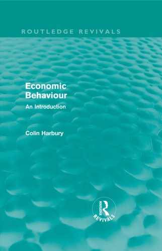
The confidence that one may have in any apparent association depends not only on the number of observations but on how varied they are. This is best explained in graphical terms as the spread, or scatter, of points around the line of best fit. Figure 11.3 shows two scatter diagrams each of which may be compared with Figure 11.2. The line of best fit in the left-hand graph, Figure 11.3 (i), is almost certainly the less reliable of the two because of the wide spread of individual observations. The line in the right-hand diagram, Figure 11.3 (ii), is deserving of less confidence because the number of observations is very small and, even though they lie exactly on a straight line, one would not be happy deriving a general rule from so small a sample.

There is no totally objective way of deciding how far one can rely on a relationship between variables which are statistically correlated. One common method used by statisticians is to consider what the likelihood is that the observed results obtained could have been obtained by chance, that is, without there being any real association between them. With a given scatter and known number of observations, it is possible to estimate the probability of this occurring. By convention, if a relationship is discovered which could have occurred only once in a hundred, or once in twenty, by pure chance, the association is described as being statistically 'significant'. It is important to stress that these are no more than conventional, arbitrary benchmarks which may be helpful in econometric work. Statistical significance is not the same as proof. We may sometimes disregard a statistically significant association, if there are grounds for suspecting that the associated variables may not be correlated.

Assessing the Results of a Test

We consider, finally, how to assess the results of confronting an economic model with empirical evidence. Three considerations arise: (1) whether an association has been established, (2) whether it is causal and (3) how general the results are.

(1) Establishing association

In order to decide whether an association between two variables has been found, one must, in the first place, judge the reliability of the correlation, that is, by examining the number of observations and their scatter. One must also look carefully at the way in which the model was formulated and the precise nature of the data used to test it, matters which were discussed earlier. If the correlation appears to be low, for example, this need not necessarily mean that no association exists, merely that it was not observed. A possible explanation might be that no time-lag was allowed for — for example, linking price to demand. A new test of a model where quantity demanded was associated with price, say, six months previously, might produce a higher correlation. There could of course also be data deficiencies (of types mentioned earlier) which precluded the test being a sound one. Moreover, the model might be too simple and exclude, by ceteris paribus assumptions, explanatory variables which exerted changed influences while they were assumed constant. For instance, the general level of incomes might have risen increasing demand and concealing, in whole or in part, an association between price and quantity.

The argument in this section warns us not to reject a hypothesis simply because the evidence from a test does not confirm it. The moral should be to subject the model to further tests if there is any reason to believe that it may still be a valid one. Much the same is true of correlations which appear to support a theory. The results are, in principle, just as capable of being due to similar errors. They should be treated with equal caution.⁵

(2) Establishing causality

The most important danger to be avoided in drawing conclusions from statistical evidence is that of assuming that high correlation necessarily means that one variable causes changes in another. In the first place, the reason for the high correlation may be that there is an important excluded explanatory variable which is the true cause of the association. For example, there is a high positive correlation between the numbers of suicides and of marriages, but no one seriously believes that the relationship between them is causal. Each happens to be highly correlated with a third variable — the size of the total population, which is increasing. In this case, it is obvious that the correlation is not causal, but by no means all false 'causation' is so obvious as this example. One should add that, sometimes, an incomplete model may nevertheless be useful, as long as it is used with care. For instance, it is said that a better than random way of predicting tomorrow's weather in Britain is to use a model which says that tomorrow's weather will be the same as today's. The predictive value of this hypothesis is apparently good on average. Yet it cannot forecast a single one of the important changes in weather that occur.

There is one other important source of error in inferring causality from statistical association that must be mentioned. It goes under the name of the post hoc ergo propter hoc fallacy (after the event, therefore because of it).

Even if a causal link exists between two variables there is still a problem of deciding which is the cause and which the consequence. An example of the way in which controversies can arise over causality in the presence of high statistical association is the question of the relationship between changes in the quantity of money and in the general level of prices. There is no disagreement about the high correlation itself. It will be remembered from Chapter 9, however, that there are two major schools of thought on the nature of the causal nexus. Monetarists believe that the change in the quantity of money causes the change in the general level of prices. Keynesians, in contrast, prefer the explanation of the causal sequence being, at least sometimes, the exact opposite. The statistical association cannot, by itself, prove either of them right or wrong. The importance of this point cannot be overstated. Yet it is all too frequently forgotten. To illustrate, two Cambridge economists discovered that the rate of change in prices in the UK was even more highly correlated with the incidence of dysentry in Scotland than with changes in the money supply! Of course they were not trying to argue a Scottish dysentry theory of inflation, but showing the unjustifiability of inferring causality from mere association, with a suitably absurd example.

(3) Generalising the results

The final matter to consider on drawing together the results of a test is how general they are. This is a vital consideration. If one has discovered a reliable statistical association and is satisfied about the causal chain, it may be used in helping to predict the future. There are two very real dangers to watch for. The first is that of assuming that past behaviour will be repeated, especially if it has persisted for a long time. Circumstances change and unpredictable events can exert new influences, upsetting previously established relationships. The reactions of the community to continuing inflation provide a good illustration. After many years of price stability the first appearance of inflation may not at once change economic behaviour at all. But continuous inflation tends to lead the community to expect it to persist and act accordingly.

The second trap that awaits the unwary observer who is tempted to draw general conclusions from limited data is known as the fallacy of composition. If a statement is correct for each and every member of a population, it is not necessarily correct for the population as a whole. There are many examples of the appearance of this fallacy in economics. For instance, it may easily be established that an individual cereal manufacturer can sell more of his product if he increases expenditure on advertising. But we cannot conclude that, if all cereal manufacturers increase advertising expenditure together, total sales will rise by the sum of the increases by all individual manufacturers. The extra sales of each may be achieved only at the expense of others; total demand for breakfast cereals may be unchanged.⁶

Economic ‘Laws’

We end this chapter on the methods used by economists to build and test models with an observation concerning the so-called 'economic laws' which may be propounded as a result. We should hardly find it surprising now to learn that economics has not produced as many stable laws as have the physical sciences. The validity of 'economic laws' is, in practice, difficult to establish, and they are perhaps better described as tendencies — the tendency for demand curves to slope downwards, or the tendency for consumption expenditure to increase as income rises. Such 'laws' are useful only in so far as they are supported by evidence. They do not necessarily apply to all individual cases; they may not be reliable in the ever-changing environment of a real economy; and they are in no sense, of course, inviolable.

Predictions concerning economic behaviour are, for the many reasons described in this chapter, liable to error. People sometimes scoff when economists turn out to be wrong, especially when different economists make contradictory predictions. No one should imagine that forecasting is easy, as meteorologists and doctors, for example, may witness. Economics is still a fair distance away from being able to forecast consistently and accurately the course of economic behaviour. It might be a much less interesting subject if it could.