Chapter 8
Optical Fiber Sensors

The most important application of optical fibers is undoubtedly in optical communications.

Optical fibers can be used as sensors as well, if we look at how certain parameters of propagation are affected by external perturbations. This is a very interesting niche from both the scientific and technical points of view.

In applications other than sensors, we strive for getting rid of external perturbations and make the fiber as immune as possible. In sensors, we need to make the sensitivity reproducible, and eventually try to increase it. Because we are interested in its measurement, we now call the physical perturbation a measurand.

In Optical Fiber Sensors (OFSs), the effect of a measurand may eventually be very minute, yet we are able to devise readout methods capable of responding with very high sensitivity. A very high sensitivity is actually a special feature of some configurations of OFSs, unequalled by any other approach. This is one of the reasons why OFSs have been actively studied and developed internationally by the scientific community since about the beginning of the 1980s, when the early high-quality fibers started to become available.

Perhaps the most successful example of an OFS is the FOG, which was treated in Ch.7. Many other examples of viable OFSs have been reported in the literature, and prototypes of OFSs for measuring quantities such as temperature, pressure, strain, and pollutants have been proposed and developed into commercial products.

The revenues from OFSs have been rather disappointing, however. The sensor market has fierce competition among many different technologies. The market expectation is not just for high-performance sensors, but more commonly for cheap sensors and sensors with a good price-to-performance ratio.

The new OFS technology can offer high performance, but is much more expensive than conventional sensors. Thus, optical fiber sensors have not been accepted for general-purpose applications, the domain of conventional electronic sensors. Only very special circumstances (like harsh environment, high EMI, etc.) may render the OFS acceptable, but this is just a small percentage of the rich and appealing sensor market. Thus, after twenty years of R&D efforts, only a few OFSs are left over as viable and successful.

In this chapter, we will present the fundamentals of OFSs and discuss a few selected examples of application.

More exhaustive references may be found in the copious literature on the subject [1-4].

8.1 Introduction

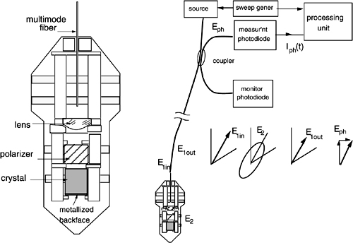
The paradigm of an OFS is shown in Fig.8-1. The measurand, through the mechanism of interaction, affects an optical parameter of the fiber.

Specifically, the optical parameter may be the intensity, or the state of polarization (SoP), or the phase of the field propagated through the fiber.

Fig.8-1 The paradigm of an OFS: the measurand, or quantity to be measured, affects an optical parameter, which is translated by a readout configuration into an electrical output.

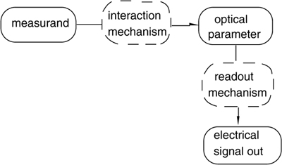
According to the parameter affected by the measurand, we arrange a readout configuration that transforms the variation of the parameter into an output electrical signal for the user.

8.1.1 OFS Classification

Sometimes the measurand is first converted by a conventional mechanism into an intermediate measurand more conveniently measured by the fiber.

Because of this difference, OFSs are accordingly classified as intrinsic or extrinsic. Another important classification of an OFS stems from the type of optical parameter involved by the interaction with the measurand.

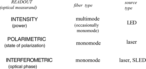
The most commonly used parameters are (i) intensity (or guided power), (ii) state of polarization (SoP), and (iii) optical phase of the propagated mode.

The corresponding readout (or OFS) is called an intensity, polarimetric or interferometric sensor (Fig.8-2). This classification is not simply nominal, as it implies a type of fiber and of source necessary to implement the readout.

Intensity readout OFS can be implemented with multimode fibers, whereas polarimetric and interferometric OFSs require a monomode fiber to preserve the interaction without the errors originated by the multimode regime.

Indeed, when many modes are allowed to propagate, each tends to collect a slightly different variation, and the modes mix generates an error.

Also, in intensity-based OFSs we do not look at the SoP nor do we need coherence. Therefore, we may use a cheap incoherent, unpolarized source like an LED. In polarimetric and interferometric OFSs, on the other hand, we need to start with a clean input field, with well-defined SoP or coherence length. We shall therefore use a laser or a SLED (super luminescent LED).

Fig.8-2 Classification of the three main readout principles and types of OFSs: intensity, polarimetric, and interferometric. Also indicated are the fibers and sources they use.

8.1.2 Outline of OFS

An outline of the most important OFSs, demonstrated in the laboratory or developed up to the level of units deployed in the field, is presented in Fig.8-3. As we can see, the range of applications is wide, spanning from mechanical to electrical to chemical quantities, and covering virtually all types of measurand.

Among the mechanical quantities, we find force, pressure, stress, strain, acoustical fields, and other derived measurands. The OFSs developed for these quantities are mostly of the intrinsic type.

Some of them are known as the optical strain gage, the fiberoptic vibrometer, and the optical hydrophone. Transducer effects used include the elastooptical effect, evanescent attenuation, and attenuation by proximity.

Fig.8-3 Outline of the most developed OFSs, with the main effect used and type of interaction.

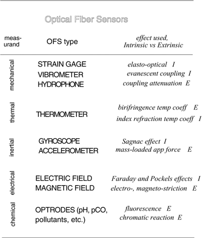
Temperature OFSs may be intrinsic as well as extrinsic. The temperature coefficient of the fiber is used for interferometric OFSs, whereas extrinsic OFSs have been developed using temperature-dependent birefringence in crystals and blackbody emission.

Electrical OFSs have been developed based either on the Faraday and Pockels effects, both intrinsic to the fiber, or occasionally on the magnetostriction and electrostriction effects, both extrinsic to the fiber.

Inertial sensors include the FOG gyroscope (see Ch.7) which is an intrinsic OFS based on the Sagnac effect, and accelerometers, which are usually realized as extrinsic, mass-loaded strain gage.

Finally, OFSs have been demonstrated for the detection and measurement of chemical species (pollutants, hydrocarbons, etc.) and for chemical quantities like pH, pO₂, etc.

Most chemical OFSs are extrinsic, and they are based on a color-developing reagent conveniently placed on the fiber tip. Because of this, a chemical OFS is also called an optrode (optical electrode).

The advantages and disadvantages of OFSs with respect to other conventional sensors derive from the fiber structure.

Because OFSs have a completely passive structure from the electrical point of view, their immunity to electromagnetic interference and chemical species is good.

They can generally withstand a high dose of radiation, in the range of Mrads compared to the 50-krads dose typical of electronic components.

Even their immunity to mechanical disturbance is generally good because of the rugged structure of the fiber.

The overall size and weight of OFSs compare favorably to other sensors and flexibility of design in shape and size is good. Frequently, OFSs are able to operate without physically contacting the measurand, or they are non-invasive.

OFSs can attain sensitivity values unequalled by other types of sensors, especially when using the most sophisticated versions, the interferometric ones.

The list of disadvantages regarding OFSs is not short, unfortunately.

To attain a high-sensitivity performance, OFSs are rather complex and expensive, whereas simple intensity-based OFSs are cheap but not so appealing in performance.

Flexibility and reconfiguration of OFSs are modest.

Ideally, the user’s requirement is an OFS composed of a readout electronic box and a probe. The electronic box (or rack-mounted panel) should be capable of performing all three readouts (intensity, polarimetric, interferometeric) with the appropriate fiber probe. In the user’s view, there should be many probes available, to perform all the measurements indicated in Fig.8-3 with a single instrument.

Unfortunately, no OFS is able to satisfy this wish list. Frequently, when an OFS is finally completed for a specified measurement objective, if the user changes the specification just a little (in sensitivity, dynamic range, or sensor placement), we need to develop a completely different solution. Thus, while the performance capability offered by OFS technology is quite powerful and should always be considered a potential solution, the range of applications outside the specification is generally quite modest and allows little or no reconfiguration.

8.2 The Optical Strain Gage: A Case Study

The field of sensors in general, and that of OFSs in particular, is characterized as being open to a variety of disparate contributions. Different from other segments of engineering, the sensor field has many possible solutions to a particular problem, which look at least technically plausible when first scrutinized.

Only after a thorough evaluation of the sensor, the most suitable solution can usually be sorted out. In addition, the best solution is frequently challenged as soon as a minor change of technology occurs.

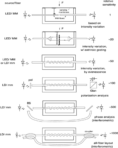
To illustrate this point, we report in Fig.8-4 an example of OFS development, that is, the optical strain gage.

This sensor has a well-known electronic counterpart, which is the resistive strain gage made of a thin film of conductive material deposited on a substrate, usually a plastic (or polymer) material. When the substrate is subjected to a stress, the film resistance changes. Arranging this resistance in a Wheatstone bridge, we can easily measure the stress or quantities connected to it (like strain, pressure, force, etc.).

Of course, the optical strain gage should offer some special feature warranting its superiority respect to the electrical strain gage if users are to prefer it.

We can start by considering a multimode-based OFS (Fig.8-4), in which two fiber pigtails are aligned in the package and one of them is actuated by a thin membrane to which external force is applied.

We can refer to this device as the reference (=1) sensitivity.

A second OFS easily follows as an extrinsic sensor when we put a grating inside the package and read the relative grating position through the fibers with collimating lenses. If the grating has black and white lines with thickness ≈2μm, compared to the 50μm of the fiber diameter, we get an improvement in sensitivity by a factor ≈25.

Further, we may think of sandwiching the fiber between two undulated jigs. If the jig is actuated in compression by the force to be measured, we induce in the fiber a curvature loss proportional to the force. The intensity-based readout of the loss is much more sensitive, perhaps by a factor ≈50 with respect to the reference scheme.

Next, we may consider reading the birefringence induced by the jig. Doing so, we get a polarimetric readout of the effect. We can use a Glan cube to separate polarization, detect the two components, and compute the ratio of the two fields to get a quantity proportional to the applied force.

As a last step to increase sensitivity, we can try measuring the optical path length variation produced in the fiber by the applied force that is, we can try converting the strain gage into an interferometric-readout OFS. We need, as illustrated in Fig.8-4, two beamsplitters to build an interferometer around the cell. The sensitivity of the interferometer readout is much larger, say about ≈500 times that of the reference configuration.

The sensor works better by removing ambient-related vibration errors. Using two fiber couplers to build the interferometer (Fig.8-4), we are able to improve the stability of the setup and accordingly the working sensitivity.

Fig.8-4 Evolution of different types of optical strain gage, through intensity, polarimetric and interferometric readouts.

8.3 Readout Configurations

Let us now consider sensor readout configurations in more detail. Our interest is assessing the basic performance of each configuration and its limits, as well as showing examples of sensors developed from the concepts.

8.3.1 Intensity Readout

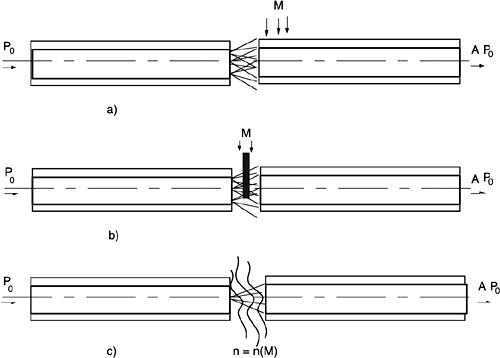
A physical measurand can affect the power propagated down the fiber in a variety of mechanisms. The most commonly used in fiber sensors are illustrated in Fig.8-5.

The measurand M may act on the position of a fiber pigtail and thus affect the alignment loss of a fiber joint (Fig.8-5a). A variant is obtained when the measurand actuates a light stop inserted between two fiber pigtails (Fig.8-5b).

In another mechanism, the measurand is related to the index of refraction n=n(M) of the medium surrounding the joint of two fiber pigtails (Fig.8-5c). A variation of the index of refraction causes the variation of the joint loss and we can read the measurand variation from it.

Fig.8-5 Different types of intensity-based sensors may use the measurand to actuate the position of a fiber pigtail in a fiber joint (a), or to exert attenuation by insertion of a light stop (b). A variation of the index of refraction, induced by allowing the measurand in the joint region, can also be read as attenuation (c).

Finally, we can take advantage of curvature-induced loss to exploit intensity readout. This can be done by mounting the fiber in a fixture with a serpentine profile of corrugation, as already considered in the example of the fiber strain-gage (Fig.8-4).

The quantity of response obtained by these transducer mechanisms can be evaluated from the alignment losses plotted in Fig.8-6 [5]. Here, loss is defined as the value of attenuation A in dB, or loss=20 log₁₀ A, where A is the ratio of output to input power (see Fig.8-5).

Three basic errors are considered in Fig.8-6: the longitudinal displacement z, the transversal displacement r, and the tilt angle α of the fiber axes. The fiber is assumed to be multimode with a core diameter 2a, and data are reported with the numerical aperture NA=[√(n ₁²-n₂²)]/n₀ ranging from 0.1 to 0.3. In the loss data, the Fresnel reflection at input/output surfaces is not included. The data of Fig.8-6 also hold true for monomode fibers at first approximation.

The case of n=n(M) can be treated, using the data in Fig.8-6, by considering that the external index of refraction n can affect the numerical aperture NA as n₀=n in this case.

Fig.8-6 Losses due to three misalignments in a joint between two fiber pigtails: longitudinal and transversal displacements and axis tilt. When more than one error is present, the total loss is the sum of individual contributions (at first approximation).

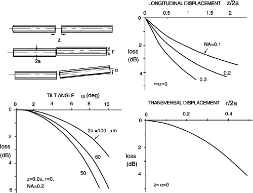
The actuation by a stop can also be treated with the displacement-loss diagrams. If we use a blade-like stop entering by a length w in the fiber gap of width g, the total loss is the sum of a transversal displacement w/2a and a longitudinal displacement g/2a loss.

Fig.8-6 is the starting point for the design of a sensor, because we can determine the displacement leading to a full signal swing as well as the linearity of response.

However, as we start developing a practical sensor design, we soon realize that the conceptual configurations of Fig.8-5 put forth several undesirable features. To illustrate this through an example, let us consider a pressure sensor developed from the blade-like stop concept (Fig.8-7).

This sensor uses two pigtails of multimode fiber (with core diameter 2a=50 or 62.5 μm), aligned by sleeves to face each other precisely, typically with a gap g=20μm. A thin diaphragm membrane is deformed by the pressure under measurement. Integral with the diaphragm, a thin blade is slipped into the gap between the fibers.

From the data of Fig.8-6, we can calculate the attenuation A=P_out/P_in of optical power passed though the sensor. This quantity is proportional to I_ph=σP_out, the current supplied by the photodiode placed at the exit fiber, σ being the spectral sensitivity of the photodiode [6].

Fig.8-7 A pressure sensor (top left) uses a fiber joint with a stop actuated by a thin diaphragm. The response curve (top right) of detected current vs. stop displacement replicates the ratio of optical power (or loss) P_out/P_in. The sensor is read by the LED/photodiode combination (bottom).

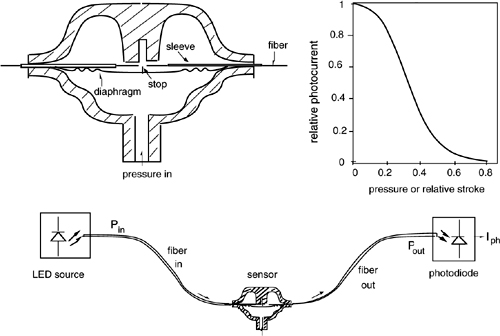
Writing P_out=AP_in and I_ph=σAP_in, we can see that the photocurrent I_ph is a good replica of attenuation A, provided the input power and spectral sensitivity are constant. Actually, both P_in and σ are likely to vary with temperature and aging. In particular, the input power will be supplied by an LED, and we should check temperature coefficient and long-term drift of input power from manufacturer’s data or by specific testing.

We may as well correct the measurement from drifts in P_in and σ, adding a circuit to compute the ratio of I_ph and P_in/σ. Of course, this would spoil the inherent simplicity and low component count of the intensity-readout approach.

An additional error affecting the scale factor is the transversal misalignment of the two fiber pigtails. If this error drifts with time, it will seriously impair the sensor response calibration further.

Another concern is the poor linearity of the pressure-to-current curve displayed in Fig.8-7 (right). We may improve linearity by limiting the range of the input pressure, but then we should require a calibration to set the working point at the middle of the dynamic range. In practice, the linearity error is not easily corrected unless we are ready to add sophistication and increase the price of the sensor substantially. Thus, we would probably end up with accepting poor linearity and limiting the sensor to the least demanding application, for example, an on/off alarm or the like.

In the design of Fig.8-7, we are using two fiber pigtails for sensor access and connection to the source (an LED) and the detector (a photodiode). Two fibers increase the cost of installation and are not that necessary. It would be better to access the sensor from just one fiber, used downstream to send optical power to the sensing region and upstream to collect the returning signal.

We may thus wish to modify the initial configuration of the intensity sensor to: (i) read in reflection; (ii) improve the linearity of response; (iii) have a self-aligned placement of the fiber. Two examples of the several possible solutions are shown in Fig.8-8.

Fig.8-8 By using the membrane diaphragm as a reflector, the pressure sensor can be read in reflection by a single fiber (left). In place of the membrane, a bellow coaxial to the fiber can be used to reduce overall size (right).

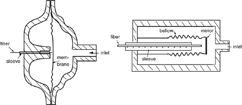
In the examples, the end-face of the multimode fiber is placed at a suitable distance z₀ in front of the membrane subjected to external pressure.

The membrane is a thin metal foil with enough reflectivity to act as a mirror for the light exiting from the fiber. In another implementation, the membrane is the cap of a bellow coaxial to the fiber (Fig.8-8 right) and overall size is shrunk to a minimum.

The downstream and upstream optical signals can be separated with the aid of a 50% fiber coupler (Fig.8-9). The coupler is the all-fiber counterpart of the bulk-optics beamsplitter. It transmits a fraction T and reflects a fraction R=1-T of incoming power. To minimize the total loss T(1-T) experienced by the go-and-return path to the sensor, we must take T=0.5 or, have a 50% coupler.

The fiber and membrane combination is equivalent to a two-fiber joint with a gap twice the distance z₀, and the diagram of attenuation due to longitudinal displacement (Fig.8-6) is still applicable using z= 2z₀.

At the output of the measurement photodiode, the response of current I_phm is found close to a negative exponential (Fig.8-9), and thus not at all linear. However, we can convert this response into a linear one by computing the logarithm of I_phm.

In this way, we get the log-attenuation A (dB), a quantity which is about linear with longitudinal displacement or input pressure, as indicated by Figs.8-6 and 8-9.

We can perform the conversion at little extra cost by using the photodiode itself as a logarithm converter (Fig.8-9). As it is well-known [7], to perform this function we shall use an op-amp follower reading the photodiode in the open-circuit mode.

Fig.8-9 The current response of the reflective readout pressure sensor is a negative exponential (left), but we transform it into a linear one by a logarithm conversion performed by the photodiode itself. As the circuit performs the ratio of powers P_m and P_r (right), it also corrects the measurement from drifts in LED power and photodiode sensitivity.

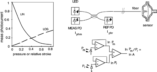
Thus, the op-amp output is proportional to the logarithm of the photodetected current [7] I_ph=σP =σ AP, and hence to the logarithm of attenuation A.

Working with a single measurement channel, however, the dependence of the log-signal from A would be readily masked by drifts in the power P emitted by the source as well as in the spectral sensitivity σ of the photodiode.

The logarithm circuit is important because it allows us to introduce a reference channel for the correction of drifts at a minor increase of circuit complexity and extra cost. As shown in Fig.8-9, we use a second photodiode at the lower port of the fiber coupler. This photodiode acts as a reference, and it yields a photocurrent I_phr=σ_rP_r=(1-T)σ_rP_LED proportional to the power emitted by the LED and to the spectral sensitivity σ_r.

The voltages v_m and v_r at the outputs of the measurement and reference branches can be written as:

(8.1)

where V₀ is a scale factor (=59.6 mV, see [7]), I_m0,r0 are the dark currents, σ_m,r are the sensitivity of the photodiodes, and P_m,r are the received powers.

By subtracting the outputs of the measurement and reference channels, we get a signal v_out given by:

(8.2)

The last term of the first line has been assumed to be a constant because we use matched photodiodes in the measurement and reference channels, and coupler transmission T is reasonably stable with aging.

In conclusion, with the log-conversion circuit we can obtain a response with a good linearity and are able to introduce a reference channel that cancels the drifts of LED and photodiode [7]. With minor modifications to the basic scheme of Fig.8-9, the concept of double-channel readout with measurement and reference for drift cancellation is utilized in a number of intensity-based sensors.

A temperature OFS based on the fluorescence of a crystal excited by an LED source is illustrated in Fig.8-10.

The crystal is a thin plate of GaAs cemented onto the fiber pigtail end-face, and we illuminate it with an LED emitting at a wavelength λ_LED below the photoelectric threshold λ_t of the GaAs material. As λ_LED<λ_t, the LED photons are absorbed by the crystal, generating electron-hole pairs. After a certain characteristic time, recombination of a pair takes place, with the emission of a fluorescence photon at wavelength λ_t.

Photons are radiated out of the crystal and a substantial fraction of them is collected by the fiber and brought back to the detector where we can measure the fluorescent power.

Fig.8-10 A temperature OFS based on fluorescence of a GaAs crystal mounted on the tip of an optical multimode fiber. The LED illuminates the thin GaAs crystal at a wavelength (λ_LED≈750 nm) of strong absorption. The crystal emits fluorescent light at a wavelength longer then λ_LED, with a precise temperature dependence of the peak wavelength (≈0.26nm/°C). The fiber guides the light emitted by the crystal back to the photodiode.

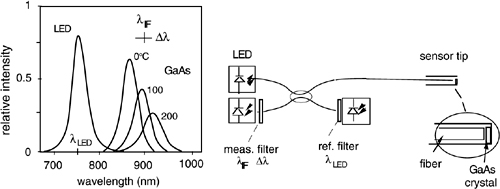
Now, both the wavelength of emission λ_t and line width of fluorescence change with temperature, as illustrated in Fig.8-10. By inserting an interference filter in front of the photodiode, with a suitable central wavelength λ_IF and bandwidth Δλ, we can maximize the response as a function of temperature and render it approximately linear.

A typical performance obtained by this approach [8] is a ≈0.2°C accuracy on a measurement range extended from –50 to +200°C.

In another approach aimed to cover a higher temperature range (0-800°C), we measure the temperature dependence of absorption α(λ) in a piece of special fiber (Fig.8-11).

The special fiber is a modified version of the normal silica fiber, prepared to withstand high temperature and to exhibit a temperature-dependent α(λ).

In an ordinary fiber, as we increase temperature, we find several failure mechanisms to fix. The first is burnout of the secondary coating, a plastic material that can’t exceed 150 to 180°C. We simply don’t use coating in the high-temperature fiber, and protect the brittle fiber tip with an appropriate end-cap. Second, at about 400 to 500°C, the silica fiber itself starts softening. We can improve mechanical resistance of the silica fiber up to ≈800°C by using quartz cladding in place of the ordinary silica cladding.

Finally, we get the desired temperature dependence of α(λ) by suitably doping the silica core. There is a variety of choices available, but a good one is Nd, the same rare-earth metal used to fabricate an optical-amplifier fiber for the 1060-nm wavelength. At a ≈0.1% concentration in the core, the Nd-doped fiber has the absorption bands shown in Fig.8-11.

Of the two absorption bands, the one at λ₁ has attenuation strongly dependent on temperature and will be the measurement channel, whereas at λ₂ attenuation is nearly independent from temperature and will be used as the reference channel.

Fig.8-11 A high-temperature OFS uses a Nd-doped fiber that has two absorption bands at λ₁ and λ₂(left): one with α(λ) strongly dependent on T, and the other nearly independent from T. Outputs from LEDs are filtered at λ₁ and λ₂, combined in the 50/50 coupler and sent to the doped fiber (right). The fiber end-face is metal-coated and reflects back the light signal to the photodiode. LEDs are pulsed in alternate phases so that both λ₁ and λ₂ channels are read by a single PD. From the PD output, a demultiplexer returns the α(λ₁) and α(λ₂) signals, from which temperature is computed.

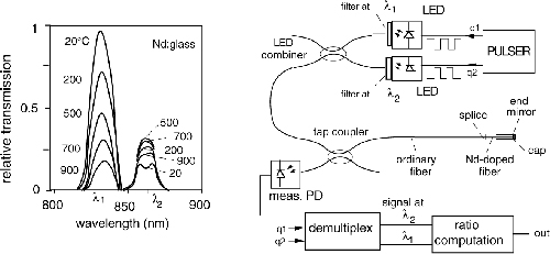
To perform the attenuation readout, we use two LEDs emitting at the central wavelength λ=850 nm and with a line width Δλ≈50 nm. By filtering the LED emission with narrow-band interference filters (for example with Δλ_IF≈ 5-10 nm), we can obtain adequate power at λ₁ and λ₂ for the measurement of attenuation at the reference and measurement wavelengths. The sensing fiber can be used in transmission or in reflection. In transmission, we need to fold back the fiber, and this operation is objectionable because the fiber without secondary coating is brittle. We may read the fiber in transmission if we metal-coat the fiber end so that it works as a mirror (as shown in Fig.8-11).

In the receiver section, we can use two photodiodes with filters at λ₁ and λ₂, or a single photodiode with a multiplex of LED sources (Fig.8-11). To perform multiplexing, we drive the LEDs in alternate phases by signals q₁ and q₂. Thus, only one LED is switched on at a time to feed the sensing fiber. When the returned signal is detected by the photodiode PD, we simply demultiplex it to the λ₁ and λ₂ channels through the phases q₁ and q₂.

Last, we can compute the quotient of the signals, usually with the aid of a logarithm converter, and obtain a signal related to temperature.

A typical performance obtained by the doped fiber OFS [8] is ≈1°C accuracy in a measurement range up to 800°C.

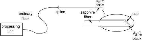
Still higher temperatures can be measured using fibers. In Ref.[9], the principle of a channel-ratio or two-color radiant sensor is described and analyzed.

Based on this concept, a radiant OFS has been developed [8]. It works on the blackbody emission of a special fiber tip, made of a multimode sapphire core and coated with alumina black acting as the blackbody surface (Fig.8-12).

The sapphire fiber is ≈10 cm long to withstand temperature, and is spliced to a normal silica fiber for the down-lead connection to the measuring instrument.

Principle of operation

The radiance per unit wavelength emitted by the fiber tip is given by the blackbody expression [9] r(λ,T)= (hc²/λ⁵)/(exp hc/λkT –1). Multiplying this quantity by the fiber acceptance AΩ, A being the area and Ω the solid angle, we get the power per unit wavelength guided by the fiber down to the detection section. We use two photodetectors, looking at two bands of the emission at wavelengths λ₁ and λ₂, and compute the ratio of their currents as: I₁/I₂=(λ₂/λ₁)⁵ exp[hc/kT(1/λ₁–1/λ₂)] (Δλ₁/Δλ₂). Taking the inverse logarithm of this ratio, we get a quantity [ln I₁/I₂]^-1=C_a+C_bT, where C_a and C_bT are instrument constants. This quantity is linearly related to absolute temperature T without the need for any calibration, at least in principle.

The operating range of the radiant-emission OFS is 500 to 2000°C, the typical resolution is ≈0.05°C, and the accuracy is about 0.5°C.

Fig.8-12 This OFS for temperature measurements in the range 500 to 2000°C employs a temperature-resistant sapphire fiber coated with alumina black. The fiber tip emits blackbody radiation, and power collected by the fiber is sent to the two-color processing unit.

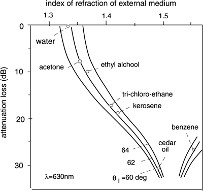
In the field of chemical OFSs, a simple sorter of chemical species is readily implemented by a multimode fiber exposed to the surrounding environment [10,11]. To accomplish this, we remove the clad from a piece of fiber of suitable length (usually ≈10 cm is enough). The external medium determines the local numerical aperture NA=√(n₁²-n_ext²)/n₀, n_ext being the index of refraction, and hence the extra attenuation experienced by the fiber tip.

The attenuation depends on the angle θ₁ under which the source launches light in the fiber, the maximum value being that of fiber acceptance sin θ₁ = √(n₁²-n₂²)/n₀. Light launched at angles θ between θ₁ and θ_ext = sin^-1NA is no more guided and the corresponding attenuation is a function of n_ext.

The typical attenuation read by a multimode OFS is shown in Fig.8-13 for several chemicals of interest in pollution monitoring. Attenuation can be read in reflection or transmission with the help of one of the several readout schemes discussed so far for intensity sensors.

Regarding this application, we actually get a large measurable signal from most species, as shown in Fig.8-13. However, we have no means to discriminate one substance from another, or, the measurement has no selectivity to species.

Fig.8-13 Transmission loss produced by an external liquid surrounding an un-coated silica fiber, as a function of the index of refraction and with the angle of launch θ₁ as a parameter.

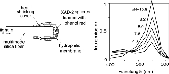
Another OFS used for measuring of chemical quantities is based on the optical change undergone by a special fiber tip, called optrode (a contraction of optical electrode). As exemplified in Fig.8-14, the optrode is made of a thin layer of a polymer incorporating a reactant substance. The reactant may change either its spectral attenuation or the fluorescence response when exposed to the chemical species under measurement.

For example, to measure the pH or acidity of a solution, the polymer layer is made of XAD-2 microspheres, treated for adsorption of phenol red.

Phenol red has a peak of absorption at λ=560 nm, which is strongly dependent on the pH, whereas at λ=475 nm we find a nearly constant attenuation (Fig.8-14).

Thus, we can measure the phenol red optrode with the aid of a scheme similar to that of Fig.8-11, and obtain a quantity related to the relative attenuation.

After a calibration, the pH is read with an accuracy of ≈0.02 in the range 6.8 to 7.9, and reproducibility is good. The measurement time is relatively long, about 60 s, because the external medium shall diffuse through the boundary membrane before coming in contact with the reactant.

Fig.8-14 A pH optrode has its fiber tip covered with polymer microspheres (XAD-2) bearing the reactant phenol red (left). The absorption spectrum of phenol red shows peak sensitivity to pH at λ≈550 nm, and a reference at λ≈475 nm (nearly independent from pH).

Another reactant used for a somewhat wider range of measurement is bromothymol blue, a dye that has a maximum variation of absorption at λ=620 nm and a minimum at λ=500 nm. With it, a pH optrode has been developed for the measurement range 6.4 to 7.8. A number of other chemical quantities can be measured with optrodes [12]. They are pO₂, pCO₂, and a number of water pollutants like pesticides, hydrocarbons, heavy metals, etc.

For biomedical use, additional applications of OFS measurement include [13,14]: glucose, metabolites, haemoglobin, breathing and blood gases [15], enzymes and co-enzymes, inhibitors, lipids, drugs, immunoproteins, etc.

8.3.2 Polarimetric Readout

In a polarimetric OFS, the transducer mechanism affects the state of polarization and we perform a polarimetric readout of the birefringence induced by the measurand.

Birefringence effects may be classified as linear or circular.

We get linear birefringence when the measurand introduces an optical retardance Φ along a (slow) axis of the fiber with respect to the other, orthogonal (fast) axis. For example, in strain and force sensors, the axis parallel to the force is the slow axis, and retardance is proportional to the force.

Linear birefringence is described as a difference in the propagation constants β_s and β_f along the slow and fast axes. Thus, down a propagation length L, we get a retardance Φ= (β_s - β_f)L.

On the other hand, we get circular birefringence (also referred to as rotatory power) when the measurand affects the direction of a linear polarization state, making it rotate while it propagates through a piece L of fiber. The angle of rotation is then Ψ=Δβ L.

Equivalently, circular birefringence can be described as retardance between right- and left-handed circular polarization states. We may then write Δβ=β_R-β_L, where β_R and β_L are the propagation constants for right- and left-handed polarizations, respectively.

Different from linear birefringence, which can only be reciprocal, circular birefringence can also be non-reciprocal. Reciprocity has to do with the change of birefringence when the direction of propagation is reversed or, propagation vector k is changed to –k.

Only two non-reciprocal effects of circular birefringence are known: the Faraday effect, which is due to a longitudinal magnetic field, and the Sagnac effect (see Sect.7.2), which is due to inertial rotation. All other effects (sugar rotatory power, crystal twist, etc.) are reciprocal, that is, rotation Ψ is unchanged when reversing the direction of observation (or the cell containing the material). Instead, reversing the direction changes rotation Ψ to -Ψ in a non-reciprocal material or medium.

8.3.2.1 Circular Birefringence Readout

Among intrinsic polarimetric sensors, we find two significant examples that have been developed to take advantage of circular birefringence effects.

The first OFS is the torsion-bar balance, based on the reciprocal rotation induced by a twist of the fiber. The twist is applied by the small weight to be measured. Because we are able to resolve an angle of polarization rotation as small as ≈10^-4 rad, the resulting OFS is a very sensitive balance, capable of appreciating a very small torque applied to the fiber (down to ≈μg·cm).

The second OFS is a magnetic field or electrical current sensor, and is based on non-reciprocal rotation. In the following, we refer to this sensor to explain the readout of circular birefringence. However, the concept also holds for the readout of reciprocal circular birefringence as well as for extrinsic sensors.

Non-reciprocal rotation is also called the Faraday effect, and it is induced by the longitudinal component H_l of magnetic field applied to the fiber. The angle of rotation Ψ is proportional to the line integral of the field H_l along the propagation path. The elemental contribution is H₁dl = H·dl, where the dot · indicates the scalar product of vectors H and dl. The constant of proportionality V is called the Verdet constant.

Thus, we may write the rotation angle as [16]:

(8.3)

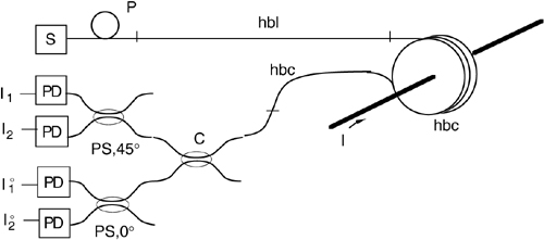
Fig.8-15 A piece of fiber or a coil can be used in connection with a polarized source S and a detector analyzer D to sense the Faraday rotation Ψ induced by a magnetic field. In a), with Ψ we read the field ∫H· dl, averaged along the fiber length. If the fiber has a mirrored end, the rotation doubles because it is non-reciprocal. With a fiber coil, rotation is proportional to the concatenated current I. Therefore in c), Ψ is proportional to the current I in the concatenated wire, whereas in d) Ψ is exactly zero.

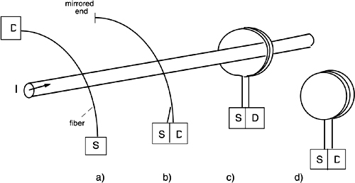
Using a piece of fiber to sense the Faraday rotation, we get a magnetic field OFS (Fig.8-15a). Indeed, in this case, rotation Ψ is proportional to the magnetic field ∫_L H·dl averaged along the fiber length L.

Using a mirrored end (Fig.8-15b) on the fiber, we fold back the propagation and get twice the rotation because the Faraday circular birefringence is non-reciprocal. By contrast, applying the fiber a twist-induced, reciprocal circular birefringence, we get rotations with opposite signs along a go-and-return path, and total effect is zero.

With a fiber coil wound around the conductor (Fig.8-15c), the OFS is a true current sensor because the rotation becomes the circulation of magnetic field intensity. This quantity is known from elementary magnetism to be equal to the magneto-motive force, that is, ∫_L H·dl = N_f I. Thus, if we arrange the sensor in the form of a winding of N_f turns of fiber wound around an electrical conductor carrying a current I, Eq.8.3 becomes:

(8.3’)

It is interesting to note that the result holds independently from coil size or shape, the only requirement being that the coil is linked to the conductor carrying the current I.

Also, if the coil is not linked to the conductor (Fig.8-15d), the rotation Ψ is exactly zero.

This feature is very attractive for the application of the current OFS to three-phase power lines [16]. Here, the three wires are close and the sensor of each phase must be sensitive only to the current carried by its conductor and not to others.

For the readout of either reciprocal or non-reciprocal rotation, we can use the general scheme illustrated in Fig.8-16.

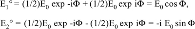
Fig.8-16 Schematic for the readout of circular birefringence. The input state of polarization E₀ is rotated by a small angle Ψ=Ψ(M) by the measurand M. The Glan cube analyzer is oriented at 45° with respect to E₀, and splits the output field into components E₁ and E₂. The photodiodes provide output currents proportional to E₁² and E₂².

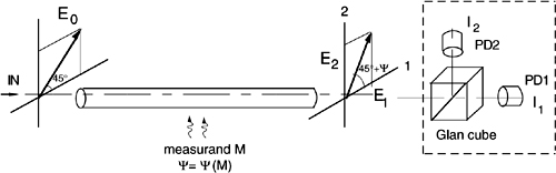
In this scheme, the fiber is read with a linearly polarized state, which can be shown [17] to be the optimal choice. As a reference system, let us take the axes (1 and 2 in Fig.8-16) of the output analyzer (the Glan cube), and assume that the input field E₀ is oriented at 45°. Along the fiber, the measurand M produces a rotation of the state of polarization, and the output field emerges from the fiber rotated by an extra angle Ψ=Ψ(M) added to the initial 45°, ending up oriented at 45°+Ψ.

The Glan cube divides the output field in the components E₁ and E₂, and directs them on two separate photodiodes, PD1 and PD2. We may then write the fields E₁ and E₂ and the associated currents I₁ and I₂ as:

(8.4)

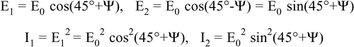
As we can see from Eq.8.4, neither the fields nor the currents are linearly related to the measurand. To obtain a better response, we compute the ratio S of difference I₁-I₂ to sum I₁+I₂ of the detected currents. Doing so, we obtain the following with easy algebra:

(8.5)

Eq.8.5 is a good result because, with the difference-to-sum ratio, we have obtained a signal linearly related to the measurand Ψ [sin2Ψ≈2Ψ for small Ψ].

In addition, the measurement is no longer dependent on E₀², the power of the input beam. In other words, the common-mode fluctuations are eliminated thanks to the ratio-like structure of the signal S.

The range of linearity may also be improved further by computing the rotation angle as 2Ψ=arcsin S ≈ S+S²/6. However, this correction does not affect the measurement ambiguity that we encounter in the sine function when the rotation angle becomes large (2Ψ>π/2).

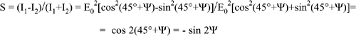
Similar to the treatment of interferometer signals, we need to supplement the measurement channel of Fig.8-16 with a second measurement channel to remove the ambiguity. This way, we make two orthogonal signals of the type sin2Ψ and cos2Ψ available.

We can obtain the second channel by deriving a fraction of the output and analyzing it through a Glan cube oriented at 0° and 45° with respect to the direction of the input state of polarization, as illustrated in Fig.8-17.

Fig.8-17 By using two Glan-cube analyzers of the output state of polarization, we can generate two signals, sin 2Ψ and cos 2Ψ, which allow us to compute the angle Ψ without ambiguity, also for Ψ>π/2.

Repeating the arguments leading to Eq.8.4 for signals E₁° and E₂° of the second channel, we can write:

(8.6)

The functions indicated in Fig.8-17 can be implemented with the all-fiber technology, as shown in the schematic of Fig.8-18. In it, we use a normal coupler C (polarization-insensitive) as the main divider of the output signal, and polarization-splitter couplers PS as the all-fiber versions of the Glan cube.

The fiber used in the coil and in the down-lead trunks is critical and requires brief discussion. In the coil, the bend of the fiber introduces linear birefringence that interferes with the small Faraday rotation. To quench the linear birefringence, a larger circular birefringence is added to the fiber of the sensing coil. This is done by twisting the fiber [16] with an appropriate period of twist (typically ≈1-3 cm). The obtained fiber is classified as high circular birefringence (hbc). It adds a reciprocal rotation Φ_rec to the useful Faraday rotation Ψ. This is not a problem with ac currents, however, because Φ_rec is a constant term and can be filtered out in the detected signal.

The same hbc fiber can also be used in the down-lead trunks connecting the coil to the instrument. Finally, in the upgoing lead, we can use a high linear birefringence fiber (hbl) in place of the hbc, as the hbl fiber is more insensitive to bends. [We can’t use the hbl fiber in the downgoing lead, because the state of polarization out of light from the coil is unknown].

Fig.8-18 An all-fiber circuit for the measurement of circular birefringence. Light from source S is polarized by fiber polarizer P and sent up to the sensing coil through the high linear-birefringence (hbl) fiber to maintain polarization. The down-lead fiber is made of high circular-birefringence (hbc) fiber. Coupler C splits the output at 50% for analyzers PS. Analyzers are polarization-splitting couplers with slow axes oriented at 0° and 45°.

A final improvement to the all-fiber scheme of Fig.8-18 is to take advantage of the difference in reciprocity of the terms Φ_rec and Ψ. If we are able to cancel out Φ_rec, operation of the current sensor is extended down to the dc component. The reciprocal rotation Φ_rec of hbc fiber pieces is actually subtracted if we trace back propagation through the fiber, whereas the non-reciprocal rotation Ψ is doubled.

Fig.8-19 With a fiber coil ending on a mirrored end, we are able to cancel out the static rotation due to circular birefringence of the hbc fiber and extend the current measurement down to the dc component.

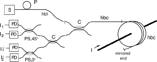
As shown in Fig.8-19, we obtain this condition by using a mirrored fiber coil end, reflecting back the radiation at the coil exit [16].

Developing the concept further, we might think of canceling the residual linear birefringence of the coil and access lead.

This can indeed be done using a Faraday mirror at the exit of the coil, in place of the normal plane mirror obtained by metal coating the fiber end face (Fig.8-19).

The Faraday mirror is a device combining a 45° Faraday rotator and a mirror. The rotator is simply made of a YIG crystal exposed to a magnetic field [16,18] that provides a non-reciprocal 45° rotation. Because of the total 90° rotation on reflection at the Faraday mirror, any input state of polarization is turned into its orthogonal on the Poincaré sphere [17]. Then, the go-and-return net change of state of polarization is zero, provided the effects generating the polarization changes are reciprocal. Therefore, all the linear and circular (reciprocal) birefringences are canceled out.

Unfortunately, cancellation does not affect the quenching effect discussed previously, and thus an eventual Faraday mirror can’t free us from using the hbc fiber in the sensing coil to contrast bending birefringence [16].

Going back to consider the signals S and S°, we can reconstruct argument Ψ and current I also for large values of rotation (>2π). The processing of signals may be either analog or digital, as outlined in Fig.8-20.

In the analogue approach, we use the same method discussed in Sect.4.5.2.3 to process the sinΨ and cosΨ signals of an interferometer. We compute the derivatives of both signals, cross-multiply them with the other signal, and subtract the result. In this way (Eq.4.39), we obtain dΨ/dt and, after a final integration, the desired Ψ proportional to current I.

While relatively cheap to implement, the analog approach has some limitations at very small signals as the errors due to the analog multiplier become important. In addition, at low frequency (or in dc), the low-pass function of the derivative is not exactly canceled out by the final integration and a low frequency cutoff remains.

Fig.8-20 Analog (top) and digital (bottom) processing of photodetected currents to obtain rotation angle Ψ.

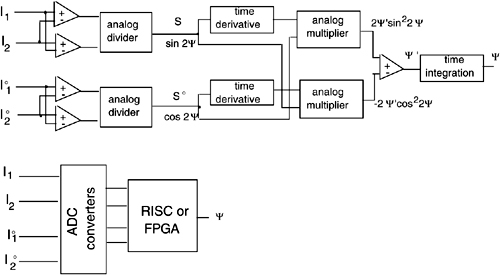
We may then prefer the digital processing (Fig.8-20), whose only limitations are associated with the offset and truncation errors introduced by the analog-to-digital converters (ADC). A reduced instruction set microcomputer (RISC), or even a fully programmable gate array (FPGA), may be adequate to carry out the modest computational load that is required.

8.3.2.2 Performance of the Current OFS

After the measurement of currents I₁ and I₂ and the calculation of the angle 2Ψ (Eq.8.5), we shall now consider the minimum detectable signal NEI= σ_l (Noise-Equivalent Current) of the sensor. At the quantum noise limit, this quantity is given [16] by the rms phase noise (2eB/I₀)^1/2 divided by the responsivity 2VN, or:

(8.7)

In this expression, V= Ψ/NI is the Verdet constant of the material [16], expressing the specific Faraday rotation (Ψ) per unit magneto-motive force (NI), and I₀ is the photodetected current in each photodiode. The 3-dB bandwidth B of the sensor is primarily limited by the transit time τ through the coil and is given by [16]:

(8.8)

where r is the coil radius and N the number of turns.

Fig.8-21 Minimum current (or NEI) that can be detected in a Faraday rotation OFS, as a function of bandwidth B and with photodetected current I₀ as a parameter. Experimental points are shown (full circle) along with the corresponding theoretical values (open circles).

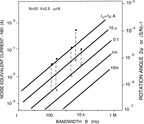
In Fig.8-21, we plot the NEI of the current OFS versus the bandwidth of measurement B, with the photodetected current I₀ as a parameter [16], as given by Eq.8.7. In the diagram, we also report the results obtained by a few research groups [19-23]. These are the dotted lines connecting the experimental results to the expected theoretical values.

As can be seen, the theoretical NEI limit due to the quantum noise associated with the readout beam is approached by about a decade, in practice. This may look like a poor result, but actually it would be very satisfactory because currents of, let’s say, 1-A can be detected with an adequate signal-to-noise ratio, up to bandwidth of ≈10 kHz.

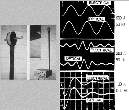
In Fig.8-22, we report the actual waveforms obtained by the Faraday current OFS and the corresponding electrical waveforms. It can be seen that they are nearly the same.

When the waveform is quasi-sinusoidal, the electrical one is delayed by 90°, and this is correct because the secondary voltage V₂=jωMI₁ lags the primary current I₁ of 90 degrees. Also shown in Fig.8-22 is the ability of the current OFS to reproduce fast transients, down to pulse widths in the range of 0.1 milliseconds or less.

Fig.8-22 A laboratory prototype of the current sensor (left) and examples of detected waveforms (right). Top traces: currents measured by a normal electrical transformer, bottom traces: currents obtained with the OFS. Top: mains current 600 A, 50 Hz; middle: a transient with 200 A peak current at 50 Hz; bottom: a fast disturbance with 10-A peak on a 0.1-ms time scale.

Another interesting application of a Faraday OFS is magnetic field sensing. In principle, we should use a single, short piece of fiber as indicated in Fig.8-15a, to get a net non-zero rotation Ψ=V ∫_L H·dl.

The Verdet constant is rather small in ordinary silica fibers (V≈2.5 μr/A at 800 nm), however. We may wish to devise some special trick to use a coil and be able cumulate the Faraday rotation on a much longer length. However, a coil unlinked to the source of the magnetic field (Fig.8-15d) has a line integral ∫_line H·dl=0.

We can take advantage of bending birefringence to have a non-zero line integral for our coil. Using an appropriate curvature radius for the winding [21,24], we may obtain a linear birefringence of 2π per turn. We need to select a ≈1-cm radius for that [25].

Then, the state of polarization changes its orientation by π each half-turn. The Faraday elemental rotation, +dΨ and –dΨ on opposite half-turns, becomes summed with the same sign and we have a total rotation Ψ=VHπr, which is only half that corresponding to the total fiber length [25].

Moreover, the two in-plane components of the magnetic field, H_x and H_y, affect the state of polarization of the bending-birefringence and Faraday rotation coil in a different way.

Thus, with a proper processing of the optical signal out of the coil, we are able to measure both of them with a single sensor [25].

8.3.2.3 Linear Birefringence Readout

Several intrinsic and extrinsic OFSs are based on linear birefringence effects. Indeed, silica in the fiber and other optical materials are sensitive to external mechanical perturbations, such as compression and bending. This circumstance leads to the development of OFSs for mechanical measurands (Fig.8-3). In addition, birefringent crystals like lithium niobate (LiNbO₃) exhibit a significant and reproducible temperature coefficient, and based on that, a temperature OFS can be developed.

Through the elasto-optical effect, mechanical perturbations are translated into linear birefringence. As it is well known, linear birefringence consists in an optical delay Φ between the linear state of polarization propagating along fast and slow axes.

The optical delay or phase shift Φ is proportional to the measurand modulus, at least at small levels of perturbation, and the axes of birefringence are normally parallel and perpendicular to the axis along which the measurand is applied (Fig.8-23).

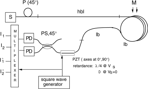
The basic scheme for the readout of linear birefringence is shown in Fig.8-23. Light from the source enters the fiber with a linear state of polarization, oriented at 45° with respect to the birefringence axes set by the measurand, that is, the x and y axes.

Fig.8-23 Schematic for the readout of linear birefringence. We enter the fiber with two equal components on the xy axes, using a linear polarization E₀ oriented at 45°. The measurand introduces a delay +Φ and -Φ between the components. At the fiber exit, we place a quarter wave plate for an additional +45° and –45° delay. We then analyze the field components E₁ and E₂ by means of a Glan cube, with the axes oriented at 45° and 135°.

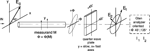
At the fiber output, the two polarization components are phase shifted by +Φ and -Φ. Thus, light emerges from the fiber with an elliptical state of polarization.

Before analyzing the state of polarization, we insert a quarter-wave (λ/4, or 45° birefringence) plate with the principal axes oriented along x and y. This way, the total phase shift between the two components becomes +45°+Φ and -45-Φ.

Next, we analyze the output field with a Glan cube beam splitter, with the axes oriented at 45° and 135° in the x-y reference, that is, parallel and perpendicular to input field E₀. To write the two field components E₁ and E₂ supplied to the Glan cube, we note that the input field feeds with two equal amplitudes E₀/√2 the x and y components. These components are phase-shifted by 45°+Φ and -45°-Φ as indicated in Fig.8-23, and then projected on the 45° and 135° axes. Adding the two contributions from the x and y axis, the fields of E₁ and E₂ are written as follows:

(8.9)

In the above equations, the factor of 1/2 in the amplitude comes from the double projection on x and y, and on 45° and 135° of the initial component E₀. In addition, to simplify the algebra, we have written delays in a symmetrical format, using -45° and +45° in place of 0 and π/2, and -Φ and +Φ in place of 0 and 2Φ. Thus, the total phase introduced by the measurand is assumed to be 2Φ.

Associated with the fields, we get two signals, I₁ and I₂, from the photodetectors, given by the square of the field modulus or:

(8.10)

It is now easy to proceed as in Sect.8.3.2.1 to derive a quantity linearly related to the measurand phase Φ. We compute the ratio S of difference I₁-I₂ to sum I₁+I₂ of the detected currents and obtain:

(8.11)

As in the previous section, we may wish to supplement the measurement by a second orthogonal signal, cos2Φ, to remove the modulus-π ambiguity of the sine function. To accomplish this function, we take off the quarter-wave plate and analyze the output with the Glan cube, again oriented at 45° and 135° with respect to the x-y reference. We then obtain two field components, E₁° and E₂°, given by:

(8.12)

Computing the signal S°=(I₁°-I₂°)/(I₁°+I₂°) gives as a result:

(8.13)

Also for a linear birefringence OFS we can extend the range of linearity beyond 2π.

The functions indicated in Fig.8-23 and the extensions required for S and S° can be implemented in all-fiber technology, as shown in the schematic of Fig.8-24.

Fig.8-24 An all-fiber circuit for measuring linear birefringence. Light from source S is polarized by the fiber coil P at 45° with respect to the slow/fast axes of birefringence of the measurand M. Coupler C splits the output from the sensing region for the double-section analyzer. One section with the λ/4 plate and a Glan cube oriented at 45° gives the I₁ and I₂ signals for the sin2Φ term. The other section, without the λ/4 plate, gives the I₁° and I₂° signals for the cos2Φ term.

The schematic operates much like that for the readout of circular birefringence (Fig. 8-18). We need two sections for deriving the I₁, I₂ pair of signals associated with S, and the I₁°, I₂° pair associated with S°. In one section, the analysis is made after a quarter-wave phase shift, whereas in the other section, the quarter-wave is missing.

In principle, the adduction fiber should have high linear birefringence (with axes oriented at 45° and 135°) to preserve polarization, whereas the down-lead fiber is a low-birefringence (or spun) fiber and be shielded by external mechanical disturbances.

From the photodetected outputs, the processing to compute S and S° follows as outlined in Fig.8-20, and the same circuits apply.

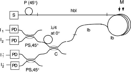
It is interesting to note that the double-section analyzer can be simplified to a single-section analyzer if we replace the λ/4 plate with a controlled phase delay device. This can be realized by a PZT (lead zirconate titanate ceramic) element with a short piece of fiber cemented on it.

When the piezo is fed by the appropriate voltage, it squeezes the fiber and introduces a linear birefringence via the elasto-optical effect. With ≈1-cm of fiber and a 1-mm thick PZT, we may need a voltage V_S≈10 V to impress the desired λ/4 birefringence. At V_S=0, the birefringence is missing and we can therefore use just a single analyzer leg, as indicated in Fig.8-25.

Fig.8-25 The linear birefringence readout can be made with a single analyzer if we use a controlled birefringence element PZT in place of the λ/4 in Fig.8-24. The PZT is driven by a square wave generator (amplitude V_S, frequency f_S = kHz) and operates in combination with a multiplexer to recover the I₁, I₂ and I₁°, I₂° signals.

The minimum amplitude of the measurand we can resolve with the linear birefringence readout depends on the responsivity Φ=Φ(M) connecting M to the phase Φ. About the phase, the minimum detectable phase or NEΦ is ultimately determined by the shot noise associated with the detected currents I₁ and I₂. Thus, we have the same NEΦ as considered in the circular birefringence readout analyzed in Sect.8.3.2.2 and plotted in the diagram of Fig.8-21 (right-hand scale).

As we can see from the diagram, limiting resolutions or NEΦ as small as 10^-5 rad are obtained experimentally and are actually representative of the state-of-the-art design. Values down to 10^-7 to 10^-6 rad are in the reach of the technique, and can be attained if bandwidth is not too demanding.

8.3.2.4 Combined Birefringence Readout

We may now wonder about the simultaneous measurement of linear and circular birefringence. In practice, it is uncommon to think of a double measurement on two measurands, one inducing circular birefringence and the other inducing linear birefringence in the same fiber. Yet, the case is one of interest as it allows us to evaluate the effect of disturbances in the sensor fiber as well as in the down-lead piece of fiber accessing the sensor.

To gain insight into this case, let us consider a fiber with two birefringences acting on the fiber (Fig.8-26), a circular one with rotation Ψ and a linear one with retardance Φ.

Let us suppose that we use the readouts illustrated in previous sections: those best suited for circular birefringence (Figs.8-16 and 8-17) and those best suited for linear birefringence (Figs.8-23 and 8-24).

Fig.8-26 The case when circular and linear birefringences are simultaneously present in the fiber.

To distinguish the signals, let us call I_1C and I_2C the outputs of the circular birefringence scheme and I_1L and I_2L those of the linear birefringence scheme.

Now, when Ψ and Φ are present, the following relations hold in all cases:

(8.14)

These equations follow from the conservation of energy in the readout schemes. In addition, with easy calculations similar to those leading to Eqs.8.6 and 8.9, and omitted here for saving space, we get:

(8.15a)

(8.15b)

(8.15c)

These expressions tell us that, if we really wish to do so, we can perform a simultaneous measurement of Ψ and Φ, putting together the readout schemes already discussed. In fact, for small values of the measurands, Ψ,Φ<<1, we get cos 2Ψ≈1 in Eq.8.15b and the difference signals are I_1C-I_2C≈-2Ψ, I_1L-I_2L≈2Φ.

An example of application of the concept is provided by Ref.[25], in which two components, H_x and H_y of the magnetic field acting on a fiber coil, are simultaneously measured thanks to the interplay of Faraday (circular) and bending (linear) birefringence.

To combine the schematic of linear and circular birefringence readout, we can take advantage of the PZT controlled-phase elements discussed above, and multiplex a single channel of polarization analysis for the entire setup. A variety of useful configurations can be developed from this concept, and we will not detail them further, leaving the effort to the reader.

8.3.2.5 An Extrinsic Polarimetric Temperature OFS

Another example of an extrinsic polarimetric OFS is provided by the measurement of temperature in the range 0..500°C, as required in the application of geothermal mining [26]. Ordinary fibers do not work well at these high temperatures, and thus the OFS must be extrinsic. A suitable crystal, like lithium niobate (LiNbO₃), is chosen to withstand the required temperature and provide a linear birefringence with a sizeable and very reproducible temperature coefficient.

By measuring the phase shift Φ= Δβ L, where Δβ=β_x-β_y is the difference of propagation constants along the principal axes x and y, and L the crystal length, we obtain a Φ=Φ(T) dependence for the measurand. Indeed, if α_Δβ = dΔβ/dT is the temperature coefficient of the birefringence, then we get Φ= Δβ L = α_Δβ ΔT L.

As illustrated in Fig.8-27, the crystal is placed in a probe at the end of a long tube running parallel to the drill in search of the geothermal poll. The tube carries the adduction fiber and may be several km long. Thus, a requirement of the system is that the fiber shall be a rugged, multimode fiber with a large (50…100 μm) core diameter, so that mechanical tolerances of the mounting are minimized. We would also like to use a single fiber for both feeding the crystal with polarized light and bringing back the useful signal to be measured.

Because the multimode fiber does not maintain polarization, we must insert a polarizer (a calcite prism) in the gauge, in front of the sensing crystal. After the optical signal coming out the LiNbO₃ crystal is properly polarized, we only need that the adduction fiber has little attenuation and a negligible polarization-dependent loss. This constraint can be amply satisfied with ordinary multimode fibers.

We now need to modify the double channel strategy illustrated in last section and look for the sinΦ and cosΦ signals from a single amplitude measurement, performed external to the probe.

This can be done by taking advantage of the wavelength dependence of birefringence, Δβ=Δβ(λ). Using a semiconductor laser diode, a wavelength sweep is easily achieved by applying a sweep to the drive current. Thus, in addition to the signal Φ, we have a time-dependent phase φ(t)= Δβ(λ) L. We manage φ(t) swings on a full 2π cycle.

The arrangement of Fig.8-27 has the crystal and the polarizer passed twice in the go-and-return path. With the arguments leading to Eq.8.9, it is easy to find the signal E_1out leaving the probe, and the result is:

(8.16)

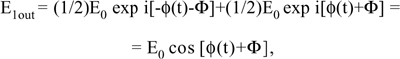
Fig.8-27 Left: layout of a temperature probe based on extrinsic linear birefringence. Light from the source is guided by the multimode fiber to the probe and passes through a polarizer oriented at 45° with respect to the LiNbO₃ principal axes. Light mirrored back from the crystal is analyzed by the polarizer itself and brought back to the detector location. Right: to recover the phase Φ of linear birefringence, the laser source is swept in frequency so that the optical path length ΔβL=φ(t) undergoes a full 2π cycle. By calibrating the crystal response, we can trace back the phase Φ=Φ(T) and hence the measurand T.

After propagation through the multimode fiber, the state of polarization of E_1out will suffer a major change, yet the total power contained will be the same E_1out² value leaving the probe.

Then, after detection, we have a current I_1ph = E₀² cos²[φ(t)+Φ] = E₀²{1+cos2[φ(t)+Φ]}/2. We may drop the constant term and consider the time-dependent signal I_1ph(td)=cos2[φ(t)+Φ]. After calibrating the system (crystal, laser diode, and sweep amplitude), we know the times at which it is φ(t)=0 and φ(t)=π/4.

By sampling the output signal I_1ph(td) at these times, we obtain the desired signals cos2Φ and cos2[π/4+Φ]=-sinΦ and we are brought back to the usual signal processing.

The measurement is incremental and we need to start with the FOS at a reference temperature (usually ambient temperature) and count the periods or fractions of them to get the current temperature. The incremental constraint is not a problem in geothermal gauging, because the drill starts from ground.

In the practical instrument [26], a resolution of 0.02°C has been achieved in the range of 0 to 500°C, while the accuracy has been estimated of better than 0.1°C.

Modifications of the concept, with the use of a polarization-maintaining fiber in the adduction trunk, have been also reported [27].

8.3.3 Interferometric Readout

In an interferometric OFS, the measurand affects the optical path length of a piece of fiber exposed to it, and we obtain the path length or phase readout by means of a suitable configuration of interferometer.

In Chapter 7, we treated in detail the best-developed interferometric OFS, the FOG. Other interferometric OFSs share with the FOG excellent sensitivity, unparalleled by other electronic sensors. A feature common to all interferometric OFSs is the remarkable sophistication of the device structure.

Because of these features, interferometric OFSs have a very appealing potentiality of performance, but their rather high cost has been a serious obstacle to market penetration.

In general, any type of optical interferometer can be virtually employed to provide a measurement and a reference arm, thus we are left to make the fiber counterpart out of the conventional bulk-optics interferometers described In Appendix A2 (see Fig.A2-1).

Fig.8-28 Commonly employed configurations of OFS interferometers are the all-fiber versions of conventional bulk-element interferometers. M and R indicate the measurement and reference arms.

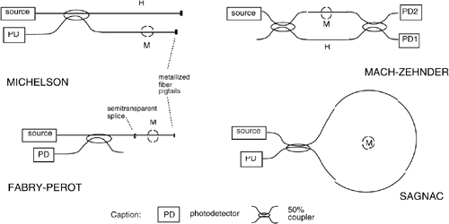
We obtain the interferometric OFS illustrated in Fig.8-28 by replacing free propagation with fiber-guided propagation, beam splitters with fiber-couplers, and mirrors with metal-coated pigtails.

Of course, if we need a well-reproducible phase of the optical field after propagation in the fiber, this shall be monomode. Then we may add some special feature, for example polarization control (the hi-bi fiber of the FOG), dispersion control, nonlinear effects, active-ion doping, and so on, yet the basic requirements is the monomode character of the fiber. As a consequence, all the components in an interferometric OFS shall be monomode.

All the different configurations basically supply a signal of the type cosΦ. Interferometer performance differs from one configuration to another, however. As discussed in Appendix A2.1, the responsivity of the interferometer may vary from 1 (Mach-Zehnder and Sagnac) to 2 (Michelson) and to F (the finesse, >>1) in the Fabry-Perot interferometer (see Table A2-1).

In addition, a reference arm is available for the cancellation of extraneous disturbances in Michelson and Mach-Zehnder interferometers, whereas it is missing in the Fabry-Perot, and is not separately accessible in the Sagnac interferometer.

Other important features of the OFS are: the balance or unbalance of the arms, the colocation of source and detectors on the same side of the fiber, and last but not least, the retro-reflection into the source.

In view of these features, it turns out that the Mach-Zehnder configuration is best for a general-purpose OFS, when we want an easy-to-implement sensor with a readily available reference arm and no disturbance effects from retro-reflections. Additionally, the differential output (PD1 and PD2 in Fig.8-28) is useful for common mode cancellation. The price for this configuration is the increase of component count (two couplers) and the placement of the laser and detector on opposite sides of the fiber.

If we don’t want to fold the fiber to get a probe-like sensor with input and output on the same side, we may resort to the Michelson configuration. This uses a single coupler and has twice the responsivity of the Mach-Zehnder, but the dual detector can’t be fitted in, and retro-reflection may disturb the source. If the source is a laser with a coherence length larger than the go-and-return optical path length, then we need to protect the laser with an optical isolator placed at the laser output before entering the OFS fiber.

Because the isolator is a rather expensive component, we generally try to avoid it and limit the coherence length to the value strictly required, that is, the path length difference between the arms.

The Fabry-Perot is an attractive configuration when we want an OFS with the highest responsivity. In fact, a finesse up to F=50-100 can be attained in metal-coated fibers, and the improvement in response may be quite significant. Disadvantages of the configuration are (i) the criticality of metal coating required to build the cavity, and (ii) the sensitivity of the access lead to external disturbances.

The Sagnac configuration is definitely ideal when sensing a non-reciprocal effect, as already discussed in connection with the inertial rotation in the FOG and the Faraday effect in current and magnetic field sensing. For reciprocal effects, on the other hand, one cannot separately access the reference and measurement paths for disturbance cancellation.

The ultimate sensitivity of interferometric OFS can be expressed in terms of a NEM (Noise Equivalent Measurand).

If Φ=Φ(M) is the relationship connecting the measurand and the optical phase impressed to the fiber, we can write the NEM as NEM= φ_n/R_φ. Here, φ_n is the phase noise of the interferometric measurement (given by Fig.4-18), and R_φ=Φ′(M) is the phase responsivity given by the derivative of the phase respect to the measurand, calculated at the working point.

In practical OFS, we can attain phase noise φ_n in the range of 10^-7 to 10^-6 rad. Yet, these values require a careful design of both the optical layout and electronic processing. In addition, we should take into account the thermodynamic phase fluctuations of the fiber (Sect.4.4.5), as this limit is in the reach of OFSs.

8.3.3.1 Phase Responsivity to Measurands

The phase responsivity R_φ of a fiber is important to evaluate the signal that can be generated in an intrinsic OFS with interferometric readout.

Table 8-1 collects typical values that are illustrative of the responsivity of three types of fibers: (i) standard monomode fiber with standard polymer secondary coating; (ii) fiber with special coating, for enhanced sensitivity to measurand; (iii) fiber with special coating, to desensitize it to the measurand.

The reason for the three fibers is that ordinary fibers are, to our surprise, appreciably sensitive to lot of unexpected measurands.

We certainly will make our best effort to compensate for undesired measurands with the use of a reference arm, which greatly helps to desensitize it. However, the ideal sensor, sensitive only to a specific measurand and immune to any other, is surely best approached if we use special fibers.

Table 8-1 Typical Phase Responsivity of Fibers

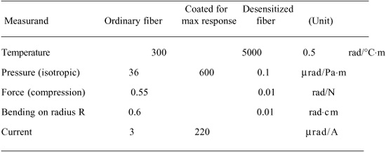
In particular, a special fiber designed for sensitivity to the measurand is useful in the OFS sensing section (the measurement arm), whereas another special fiber desensitized to the measurand is best suited for the reference section (or arm).

Finally, the piece of fiber adducting the sensing region should be desensitized to all extraneous measurands. As we can see from the typical data reported in Table 8-1, the desensitized fiber is about 2…3 decades less sensitive than the most responsive fiber. This is a good result, but perhaps not enough to seriously challenge conventional electronic sensors, that may put forward a typical cross-immunity of 10⁵ to 10⁷ to undesired measurands.

8.3.3.2 Examples of Interferometric OFS

Several interferometric OFSs have been proposed in the literature, and the most exhaustive reference on this topic is perhaps the recently prepared Collection of Optical Fiber Sensors Proceedings [28].

If we exclude the FOG, which is by far the unrivaled interferometric OFS, the most interesting OFS is the hydrophone, from the application point of view. The hydrophone is a device intended for hydrostatic pressure sensing in underwater environments.

Using a properly jacketed fiber sensitive to isotropic pressure, and laying a section of it coiled so as to cumulate the measurand on an appropriate length, we get the schematic of Fig.8-29. Here, the pressure-sensitized fiber is coiled at the end of the measurement arm of the Michelson configuration.

The reference arm brings a phase modulator (with a PZT) to adjust the quiescent working point in quadrature, so that the photodetected signal is of the form I_ph = I₀ [1+cos{Φ(M)-φ_r}] = I₀ [1+sinΦ(M)], where Φ(M) is the phase induced by hydrostatic pressure, and φ_r is the reference arm phase shift whose low-frequency (or average) component shall be dynamically locked to π/2 (compare to Fig.4-34 and Sect.4.6.1).

With several cm of coiled fiber, the sensitivity of the OFS hydrophone can reach 0 dB_a or p_a= 2·10^-5 Pa [29]. This is the reference level of acoustic pressure and corresponds to the threshold of audibility.

Fig.8-29 Schematic of an interferometric hydrophone using the Michelson readout configuration. The sensing fiber is a coil of pressure-sensitized fiber, whereas the adduction and reference arm fibers are desensitized.

Another schematic similar to that of Fig.8-29 applies to the measurement of temperature. In this case, we take advantage of the PZT modulator to perform two functions: (i) removing the ambiguity of the cosine function, and (ii) extending the resolution to a small fraction of wavelength (or 2π angle). To do so, we sample the phase of the measurand φ=Φ(M)-φ_r by three or four values of the reference φ_r. Three values are those already illustrated in Fig.4-11; some researchers prefer using four values.

For example, we may switch φ_r on a sequence of three values: 0, ..2π/3…-2π/3. By sampling the 1+cos[Φ(M)-φ_r] signal in correspondence, we triple the interferometric signal, as in the general scheme described in Sect.4.2.2.1. From the three signals, we can compute Φ(M) (see Eq.4.11) with a ≈nm resolution (equivalent to ≈π/200 rad) and get the appropriate up/down signals required for a range exceeding 2π.

Similar to an interferometer for displacement measurement, when the phase induced by the measurand exceeds 2π we count up/down transitions in a counter, and the measurement is an incremental one. To work correctly, the sensor shall be reset at an initial temperature T₀ and allowed to count the periods induced by temperature between T₀ and the current temperature T. Temperature resolutions down to 10^-4 degrees have been reported based on this configuration of interferometric OFS.

8.3.3.3 White-Light Interferometric OFS

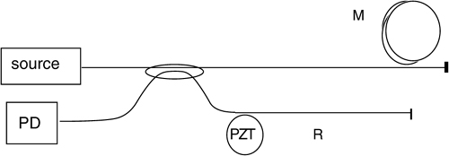
The white-light interferometer described in Sect.4.8 is readily adapted to an OFS, as illustrated by the schematic in Fig.8-30.

Fig.8-30 Schematic of a white-light interferometer OFS. Mirror M is mounted on a motorized stage, and when the arms are balanced (s_m=s_r±l_c), fringes appear.

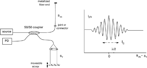
In the Michelson version of the interferometer, the arm with in-fiber propagation is used to collect the measurand phase perturbation. In the other arm, we exit from the fiber with a collimating lens and project the beam onto the moveable mirror.

When the mirror position matches the condition s_m=s_r±l_c, fringes appear and we can measure the deviation from the condition s_m=s_r looking at the fringe envelope. The resolution of this measurement is of order of the coherence length l_c (Fig.8-30).

Using a SLED source, we may typically have Δλ≈25 nm at a central wavelength λ=800 nm, and the coherence length is l_c =λ²/Δλ= 0.8²/0.025= 26 μm, a good starting value as resolution of a strain-measuring OFS. If we scan the response curve a few times and average the results, we may go down to resolve typically ≈0.2 l_c =5 μm.

This value of resolution is obtained with a very simple optical setup and needs only very limited electronic processing. Because it is cheap, the OFS lends itself to interesting application in the field of construction, called either non-destructive testing (NDT) or smart sensors.

For example, we may start with a 1-m piece of fiber, with one end-face metal-coated and the other end-face ending on a connector. The fiber is then threaded inside a steel tube and glued to it, and this constitutes an arm of the OFS. The arm duplicates the strain Δ1/1 applied by the structure external to the tube.

Now we can cast the fiber inside a concrete pillar to monitor its state of strain during the useful life of the pillar. The fiber tube is put in place while the concrete is poured to fabricate the pillar, leaving out just the connector for access.

After a period of time (e.g., months to years), we can go back to examine the sensor and check the strain applied to it and to the concrete structure. From this we get non-destructive diagnostics of the construction work. As a 10-μm resolution on a 1-m fiber length is a strain σ= Δ1/1= 10μm/1m= 10μstrain, we obtain a sensor amply capable of diagnosing incipient overload of the structure (usually found at 100…1000 μstrain).

About disturbances, temperature variations may actually affect the measurement of strain. Indeed, a typical sensitivity (Table 8-1) of 300 rad/°C·m amounts to about 300/2π≈50 wavelength/°C. At λ=0.8μm, this quantity corresponds to a strain equivalent of 50·0.8= 40μm/°C·1m = 40 μstrain/°C.

However, we can measure the temperature of the pillar and correct against thermal drift and associated errors if we characterize the response prior to installing the fiber.

The white-light approach is interesting and has led to successful products. Its only drawback is the mechanical scanning of the reference path with the moveable mirror.

8.3.3.4 Coherence-Assisted Readout

A more elegant configuration of a white-light interferometer can be devised starting from the idea that, casting in the experiment a full interferometer instead of just the measurement arm, we make available a reference to subtract the undesired disturbances.

To do so, we shall read the path length difference s_mS-s_rS, between the measurement s_mS and reference s_rS paths contained in the sensing (S) section of the item under test.

For the subtraction, we secure the measurement fiber to the enclosure tube and leave the reference fiber loose. Thus, the difference s_mS-s_rS is sensitive to the measurand as before, whereas temperature and other common mode disturbances are canceled out.

Now, the problem is how to read the s_m-s_r difference having already used both arms. With a white-light interferometer, we have one more degree of freedom available, which is coherence.

Thus, we develop a coherence-assisted readout as shown in Fig.8-31.

In this scheme, we use two interferometers in series, in the sensing (S) and readout (R) section. We make the path lengths s_mS and s_rS differ by several coherence lengths l_c of the source so that the output fields from these arms will not beat at the photodetector. For example, we typically let s_mS-s_rS=Δ≈ 20·l_c ≈ 0.5 mm, for arms s_mS, s_rS≈1-m long.

In the readout section, we work with the same nominal lengths of the reference and measurement paths. For simplicity, let us take identical reference lengths s_rR=s_rS. Then, scanning the measurement path s_mR with the moveable mirror, we will find the readout interferometer in the same imbalance of the sensing interferometer when we reach s_mR=s_mS.

This condition corresponds to the balance of two special paths in the optical setup. One passes through the measurement arm of the sensing section and the reference arm of the readout section with a length s_mS+s_rR. The other passes through the reference arm of the sensing section and the measurement arm of the readout section with a length s_rS+s_mR. Along these two paths, the electric fields collect a phase delay 2k(s_mS+s_rR) and 2k(s_rS+s_mR), respectively.

When the two fields are collected at the receiver, they generate the following photodetected signal:

Fig.8-31 An optical fiber sensor using coherence-assisted readout employs two interferometer sections for sensing (S) and readout (R). The arm lengths of the interferometers differ by a quantity Δ much larger than the coherence length l_c. The moveable mirror is scanned, and when position s_mR= s_rR+(s_mS–s_rS) is reached, white-light fringes appear as in Fig.8-30.

(8.17)

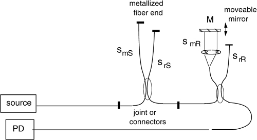
With a coherence length l_c, interferometric fringes similar to those of Fig.8-30 are generated in the interval s_mR=s_mS+(s_rR-s_rS)±l_c of moveable mirror position.

When the reference paths are identical (s_rR=s_rS), this gives s_mR=s_mS±l_c.

As there are four possible paths in the double interferometer schematic of Fig.8-31, we shall also examine the additional terms beating at the photodetector. These terms are easily found by writing the amplitude and phase of the field propagating down the fiber circuit in Fig.8-31. Developing the calculation, we find the additional terms and write the total current at the photodetector as:

(8.18)

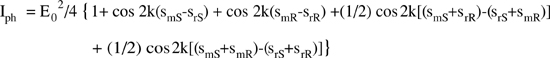
The first term in curl brackets has a zero mean value because the argument, s_mS-s_rS≈Δ, is much larger than coherence length. The second term can give a fringe pattern, but only when s_mR-s_rR≈± l_c. We never get it, because the difference s_mR-s_rR is about equal to s_mS-s_rS≈Δ. Thus the second term has a zero mean value, too. The third term is the desired one, beating for s_mR-s_mS≈±l_c. The last term has a beat only for s_mS-s_mR≈-2Δ, or it has zero mean value.

In conclusion, the extra terms may contribute with their beatings as well, but far away from the main one if we keep Δ>>l_c, and we can easily reject them in the course of the scan.

Once we have been able to compensate the interferometer from thermal and other undesired drifts, we can push the resolution further. Indeed, when the white-light fringes are still under the envelope waveform, we can look for the one with the largest amplitude.

This is the central fringe, defined by position to the usual λ/2-displacement per period. Therefore, if we look at the central fringe we get a resolution of about 0.5μm, or 20 times better than the envelope (or coherence-based) position-sorting.

Important to note is that, near the balance condition, the white-light interferometer behaves exactly like a conventional interferometer, and its ultimate limits of performance are those already discussed in Sect.4.4. Thus, nm-resolution is also achievable.

8.4 Multiplexed And Distributed OFSs

Despite the generally excellent technical performances of OFSs, their relatively high cost has so far prevented their widespread use in applications, especially in comparison with conventional electronic sensors.

One way to get around this problem is to offer a number of measurement points instead of a single point. We can multiply the number of measurement points substantially, either by allowing the measurement to be distributed in space or by multiplexing a number of individual sensors on the same line served by a single readout unit.

If the approach is to become the winning breakthrough, the cost of multiplexing or distributing the sensors should be low, about a fraction of the total OFS cost.

Several approaches have been studied through the years to provide a viable approach to the multiplexed or distributed architecture, and copious literature has been published on the subject [28,30,31].

8.4.1 Multiplexing

Multiplexing may be implemented by several methods; the most popular are (i) space-division; (ii) time-division; (iii) wavelength-division; and (iv) coherence-division.

Space-division uses a switch connecting each individual sensor to the readout unit. Each sensor is read in sequence, one right after the other. Because of cost requirements, the switch is usually a mechanical rotary device, and the operation time (switching from one sensor to the other) is about a few milliseconds.

For faster response, we may use a more sophisticated approach: for example, we may start with a Mach-Zehnder waveguide interferometer realized in LiNbO₃ or in silica-on-silicon (SoS). These are 2-way switches, connecting the input guide to one of the two output guides, and are actuated by an electrical signal applied to the control electrode. By arranging N stages in cascade, we realize a 1×2^N switch array. Price becomes prohibitively large at increasing N, however, and this solution is limited in practice to, say, N≤4.

Time-division implies the use of a short-pulse laser source to interrogate sensors, which are located down a fiber at different lengths from the source. For example, Fig.8-32 shows an example of time-division multiplexing OFS.

Called ladder configuration, this multiplexing scheme employs a pulsed light source and a series of sensors connected with couplers to common rails of fiber for feeding the sensors and for collecting the returned signals. The time duration of the pulse τ is made shorter than the extra delay 2L/c experienced by a sensor with respect to the preceding one.

Under this condition, each sensor responds with a pulse falling in a well-defined time-slot (Fig.8-32) and thus we can demultiplex the responses at the receiver.

Each coupler takes a fraction of the incoming power to its sensor. To equalize responses, the coupling factor at the n-th sensor should be chosen as k_n=1/(N-n+1), where N is the total number of multiplexed sensors. By doing so, the first sensor has k₁=1/N and leaves a through power of 1-1/N. The second sensor has k₂=1/(N-1), takes a fraction [1-1/N]/(N-1)=1/N of incoming power, and leaves a through power of [1-2/N]. The third sensor has k₃=1/(N-2) and takes a fraction [1-2/N]/(N-2)=1/N. This continues up to the N-th sensor that has k_N=1 and takes a fraction 1/N of input power.

In the return path, the fraction of power deviated onto the common rail is the same value, 1/N of the power deviated from the feed rail. Thus, with respect to addressing individual sensors, the operation of multiplexing introduces an extra attenuation 1/N².

With an appropriate design of source power and receiver sensitivity, attenuation limits the maximum number of sensors that can be multiplexed to N≈15..20.

Fig.8-32 Time-division multiplexing of an OFS, using a pulsed source and individual sensors arranged in a ladder array. To distinguish the pulses returning from individual sensors, the pulse width τ should be shorter than the delay 2L/c added at each additional stage. Extra fiber length can be added between sensors to match the condition.

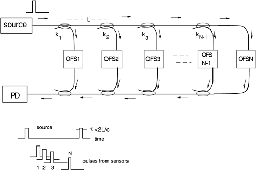
The time-division scheme has been employed for polarimetric as well as interferometric sensing [31] of temperature, strain, and acoustical emission, especially in connection with marine applications.

Wavelength-division multiplexing consists of assigning a wavelength slot to each individual sensor and reading the composite output with a narrow-band source tunable in frequency. To be suitable for cascade connection, the sensor should be frequency-selective, respond in transmission or reflection and let the out-of-band components pass unaltered in reflection or transmission.

These requirements are satisfied by Fiber Bragg-Gratings (FBGs), passive components well known in optical fiber communications. An FBG is a longitudinal grating, written along the axis of the fiber as a periodic variation Δn of the refraction index, produced by exposure to UV radiation [4].

If Λ is the spatial period of the grating, the Bragg condition 2n Λ=λ_B determines the wavelength of resonance λ_B. For wavelengths close to λ_B, the device reflects back the incoming radiation, whereas radiation off-resonance (λ≠λ_B) passes unaltered through the FBG. We summarize this behavior by saying that the FBG is a band-reject filter in transmission or a band-pass filter in reflection.

The FBG can be used as a sensor because the resonant wavelength λ_B depends in a reproducible way on temperature and strain, the two quantities most commonly measured with FBGs. The relative change of resonance wavelength is written as:

(8.19)

Here, p_e is the elasto-optic coefficient of the fiber (typically p_e≈ 0.22 for silica), κ=α+Ψ is the total thermooptic coefficient (typ. κ≈5·10^-6 in silica), and ε=Δ1/1 is the strain applied to the FBG.

Fig.8-33 An FBG reflects the wavelengths close to the resonant wavelength λ_B and transmits the rest of the spectrum (top). A wavelength-multiplexed OFS is arranged by cascading a number of FBGs at different wavelengths λ_B and using a tunable laser source for reading the individual sensors.

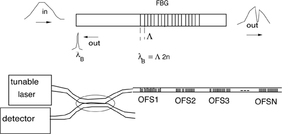
Connecting a number of FBGs in series, as indicated in Fig.8-33, we get a wavelength-multiplexed sensor. The array can be read by a wavelength-tunable laser source because each FBG other than the selected one is transparent, whereas the sensor interrogated by the laser source will respond with a peak reflection in correspondence to its resonant frequency.

The shift in wavelength resonance Δλ_B is dependent on temperature T and strain ε applied to the FBG. If we are to avoid cross-sensitivity to T when measuring ε, or vice versa, we should use a pair of FBGs, arranged in the experiment to have different sensitivity to T and ε. By combining the results of the measurements in a set of two equations, we can solve for both (T and ε) measurands.

A feature that is unsatisfactory in the ε-multiplexed sensor of Fig.8-33 is the use of a wavelength-tunable laser source. This is an expensive item and, if it is the only possibility, it is likely that an OFS incorporating it will hardly leave the laboratory.

Thus, we may want to modify the concept of λ-multiplexed readout. One of the several solutions reported in the literature is shown in Fig.8-34. Here, we use a broadband source to illuminate the sensors and duplicate each FBG in the sensing chain with another FBG in the measurement chain, with nominally the same resonant wavelength λ_B.

Fig.8-34 Schematic of a λ-multiplexed sensor that uses two sets of FBGs in the measurement and reference chain. Corresponding OFSs have nominally identical resonant wavelengths λ_B. The signal returning from the measurement OFS is brought to the reference OFS for response comparison. Modulating the reference λ_B with the piezo actuator allows us to demultiply the responses of individual sensors.

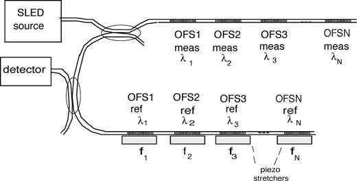
Upon application of the measurands, the k-th sensor changes its resonance wavelength by, say, a deviation Δλ_Bk. To measure the set of all Δλ_Bk simultaneously, we apply to each k-th FBG of the reference chain a stress appropriate to produce the same Δλ_Bk shift of the corresponding FBG in the measurement chain. This is done by the piezo actuators, the PZT slabs stretching the fiber of each FBG (Fig.8-34).

To operate all sensors independently, each k-th piezo is actuated with a different electrical modulation frequency f_k. The photodetector output is filtered in k bands, centered at the f_k resonance, and in each band, we look for the maximum response of the k-th FBG sensor.

Finally, coherence-multiplexing is an interesting technique that has been recently proposed. We may think of it as a generalization of the concepts discussed in Sect.8.3.3.4.

As illustrated in Fig.8-35, we can multiplex several interferometers (for example, Mach-Zehnder interferometers) by using a different arm imbalance in each OFS, and by arranging all of them in a double chain, one for sensing and the other for readout.

In the interferometers, we let the imbalance be much larger than the coherence length l_c, that is, L_k-l_k >>l_c. In addition, we let the imbalance of consecutive sensors be larger than the coherence length L_k -L_k-1>>l_c. At each detector, say the k-th of the sensing section, we find the superposition of many field contributions propagated through different paths across the interferometers. All of them are unbalanced by more than the coherence length l_c, except the two that go through the corresponding k, OFSk and Rk, in a crossed fashion, that is, l_k(OFS)+L_k(R) and L_k(OFS)+l_k(R), and share the same path in the other interferometers.

Thus, we can simultaneously read all the multiplexed sensors because the beating is returned only at the appropriate interferometer.

Coherence is an elegant solution for multiplexing, but the drawback is a large attenuation.

Fig.8-35 Schematic of a coherence-multiplexed OFS. Light from a low-coherence source is passed through a cascade of interferometers with different arm-length imbalance. In the readout section, light is split by means of couplers to a corresponding number of interferometers, duplicating the arm imbalance of the sensing section. The cross-path through the sensing and readout interferometers returns the useful signal.

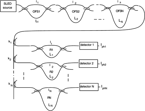
First, we shall equalize the channel amplitudes by choosing k_n=1/(N-n+1) as in the time-division scheme (Fig.8-32), and this causes an attenuation of 1/N.

In addition, at each interferometer of the sensing section, we waste a factor of 2 because of the unused ports, and this is an extra 2^N attenuation. In practice, we can hardly go beyond N≈4 unless we introduce a costly optical amplifier.

In conclusion, when designing new systems we shall use the concept of multiplexing whenever possible to reduce the cost per point. But, the total cost of the array keeps high anyway. Because complexity increases with N, a practical limit of maximum number of points comes out. Thus, we are not really gaining new segment of the sensor market by multiplexing.

8.4.2 Distributed Sensors

If we are able to read an optical parameter of a fiber resolved in distance, then each interval we resolve defines an individual sensor and a measurement point for what becomes a distributed sensor. Most of the optical parameters we use for sensing are position-dependent. In other words, fibers are born essentially as distributed sensors, but we usually make an averaged or cumulative reading of the optical parameter affected by the measurand.

From the application point of view, distributed sensors offer a decisive advantage with respect to sensors based on conventional technologies. They can be regarded as an extreme form of multiplexed sensors in that a single readout apparatus serves to measure an arbitrarily large number of individual sensing points. The cost per point of a distributed sensor then really decreases as 1/N.

Even more important, we can develop a sensor with a very large number of points, many more than is reasonable with multiplexed sensors. This feature is unequalled by conventional technology and is a great advantage in applications.

In a distributed sensor, we should be able to remotely interrogate the fiber and have a parameter telling us the distance of the fiber piece being measured. Then we should read the measurand through an optical parameter and a readout scheme (Sect.8.3). Common measurands are strain and temperature, and common optical parameters are intensity and SOP of light scattered at the individual sensing point.

Several approaches have been reported in the literature [1-4] for the interrogation of distributed sensors, namely time-domain, frequency-domain, and coherence-domain.

The time-domain approach is readily adapted to sensing because it takes advantage of instrumentation and measurement techniques [32] developed in optical fiber communication, for the remote testing of losses along fiber lines. The instrument for such a distributed measurement of attenuation is known as Optical Time-Domain Reflectometer (OTDR).

The OTDR has been used to sense stress and temperature in a variety of fibers since the early times of OFSs [33]. The interaction mechanisms first tested were attenuation by micro-bends to measure local stress, and temperature coefficient of the Rayleigh scattering to measure temperature. Both effects are small in ordinary silica fibers, however, and therefore special fibers (with a liquid core or doped with rare-earth elements) were tested in an attempt to improve sensitivity and resolution [33,34].

Later, variants of the basic OTDR scheme rather than fiber were able to provide the improvement. One is the Polarization OTDR (POTDR), by which we get a distance-resolved measurement of the SoP and hence of the birefringence of the fiber [34-36]. As birefringence is sensibly related to the stress imparted to the fiber, the POTDR is a powerful tool to remotely test and localize mechanical stresses in the fiber or in a pipeline, for example, to which the fiber is cemented.

The basic scheme of OTDR readout for the distributed sensing of attenuation is shown in Fig.8-36. Similar in concept to the LIDAR discussed in Sect.3.5, the OTDR uses a short pulse of power at a suitable wavelength to interrogate the fiber. Wavelength is chosen in the windows of optical fibers (850, 1300, or 1500 nm), so that attenuation is at a minimum and the range covered is at a maximum.

The source is a pulsed laser, usually a semiconductor laser driven by a fast current pulse and emitting peak powers of a few tens of mW. The source is eventually followed by a booster optical amplifier and protected by reflections from the fiber with an optical isolator.

The time duration τ_p of the pulse determines, as discussed in Sect.3.5, the spatial resolution of the OTDR measurement. Assuming that the response time T of the detector is faster than the pulse duration T<<τ_p, the resolution is given by Δz=cτ_p/2n, where n≈1.5 is the effective index of refraction of the fiber.

Fig.8-36 In a distributed fiber sensor, the local back-scattered power is read by an OTDR. The duration τ_p of the optical pulse used for interrogation determines the spatial resolution cτ_p/2n of the measurement, that is, the size of the virtual sensing element. The back-scattered signal looks the same as it does in Fig.3-26. After detection, the logarithm of the signal is computed, yielding the dependence from distributed attenuation and back-scattering.

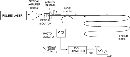
Resolutions of Δz≈1m are readily achieved with pulses of ≈10-ns duration. The quantity Δz also represents the length on which the returning signal is averaged, and thus the equivalent length of the elemental sensor provided by the distributed OFS.

The dependence from fiber attenuation α_f and back-scattering σ_bs are described by the same equations as for a LIDAR (Eqs.3.33 through 3.36), if we change the acceptance term (πD²/4z²) into the solid angle of the fiber πNA², and the neper-base attenuation in the base-10 attenuation, α =2.3 α_f.

The power in transit down the fiber is attenuated exponentially with distance z (as 10^-αz where α is the dB/km attenuation), and a fraction σ_bsdz of it is back-scattered by the elemental length dz of fiber at z. The back-scatter coefficient σ_bs(z) is dependent on the fiber material (and fiber imperfections) and on the interaction of the measurand with the fiber.

The back-scattered power returning to the source reaches the fiber coupler, and half of it is deviated to the photodiode (Fig.8-36). The detected output signal is log-converted and the result L(t) supplies the time dependence of attenuation α and the back-scattering σ_bs (Eq.3.36).

With typical powers and measurement time, an OTDR may resolve attenuation of tenths of dB, but we need a special fiber if such a resolution is to correspond to a meaningful temperature and strain range.

Alternatively, we need a different optical parameter such as polarization. The setup of Fig.8-36 becomes a POTDR by adding a polarizer in the launch section and a Stokes parameter analyzer in the detector section [37]. Using the POTDR with a normal monomode fiber at λ=1500 nm, a typical sensitivity to ≈100-μstrain with 100-m resolution can be obtained.

Fig.8-37 Spectrum of anelastic scattering with Stokes and anti-Stokes peaks located at the sides of the much larger Rayleigh peak of elastic scattering. The frequency shift Δν depends on the type of scattering.

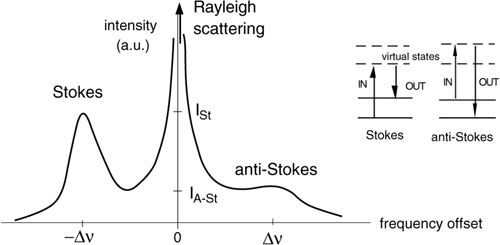
Another approach to improve performance is using a scattering different from the normal Rayleigh-Glan elastic scattering related to attenuation. Raman and Brillouin anelastic scatterings provide the desired mechanism.

These have to deal with phonon-assisted scattering, which introduces a virtual energy level in the interaction (Fig.8-37). Because of the new level, scattered radiation gains or loses a small amount of energy, E_sc=hΔν, and thus the line corresponding to scattered energy splits into two lines, separated by E_sc from the central Rayleigh-Gans (or elastic scattering) line. The upper and lower frequency lines are called Stokes and anti-Stokes lines, respectively.

Raman and Brillouin scattering differ by the energy of the phonon they interact with. The Raman effect deals with the optical phonon, relatively energetic and such that, in silica, Δν_R≈13.2 THz (or Δλ_R≈100 nm). This large frequency separation makes it relatively easy to separate the weak Raman lines from the much larger Rayleigh scatter line, a clear advantage in developing the readout instrument.

The Brillouin effect deals with the acoustic phonon and has a much smaller frequency separation (Δν_B≈11 GHz, or Δλ_R≈0.08 nm). Thus, narrowline lasers and very selective filters are required to resolve the lines.

An interesting feature of anelastic scattering is the clean and repeatable dependence from temperature of the relative amplitudes of Stokes and anti-Stokes lines. This is given by:

(8.19)

A Raman OTDR can be developed starting from the wavelength-resolved measurement of back-scattered power done at the photodetector (Fig.8-36) and by inserting suitable optical filters to sort out the Stokes lines [38]. By measuring the amplitudes of the Raman lines, temperature T can then be computed. A typical distributed sensor based on the measurement of Raman lines ratio can resolve 1°C on individual 1-m elements out of a 10-km total length of a multimode fiber, using ≈500 mW of peak power and τ_p=10 ns.

In applications, the Raman-based approach is the undisputed choice when we need distributed temperature only, because the signal is stronger and more easily sorted out.

With Brillouin lines, however, in addition to the temperature dependence given by Eq.8.19, we can also measure the frequency dependence of the separation Δν_B from strain Δl/l, a small but measurable quantity because the unperturbed Δν_B is small, too.

The dependence is written as Δν_B≈Δν_B0+ζΔl/l. In silica fibers the strain coefficient is about ζ≈ 50 (kHz/με), and Δl/l is in microstrain (με) units. An experimental setup based on the Brillouin scattering has demonstrated [39] the simultaneous distributed measurement of strain and temperature, resolving about 4°C and Δl/l≈300 με on a 15-km long fiber.

References

[1] B. Culshaw and J. Dakin, “Optical Fiber Sensors: Principles and Components” vol.1, Artech House: Norwood, MA, 1988; “Optical Fiber Sensors: Systems and Applications”, vol.2, Artech House: Norwood, MA, 1989; “Optical Fiber Sensors”, vol.3, Artech House: Norwood, MA 1996; “Optical Fiber Sensors: Applications, Analysis and Future Trends”, vol.4, Artech House: Norwood, MA, 1997.

[2] E. Udd (editor), “Fiber Optic Sensors”, J. Wiley & Sons, Chichester 1991;—, “Fiber Optic Smart Structures”, J. Wiley & Sons: Chichester, 1995.

[3] K.T.V. Grattan and B.T. Meggitt (editors), “Fiber Optic Sensor Technology”, Chapman & Hall: London, 1995.

[4] J.M. Lopez-Higuera (editor), “Handbook of Fibre Sensing Technology”, J. Wiley & Sons: Chichester, 2002.

[5] C.P. Sandbank, “Optical Fibre Communication Systems”, J. Wiley & Sons: Chichester, 1980, Chapter 3.

[6] S. Donati, “Photodetectors”, Prentice Hall: Upper Saddle River, 2000, Sect.5.2.

[7] see Ref.[6], Sect.5.3.1.3.

[8] T. Tambosso, “Fiber Optics Temperature Sensors”, Alta Freq. Riv. Elettr., vol.56 (1987), pp.143-155 (in Italian).

[9] see Ref.[6], Sect.6.3.1.

[10] M. Nagai, M. Shimitzu, and N. Ohgi, “Sensitive Liquid Sensor for Long Distance Leak Detection”, Proc. 4^th Intl. Conf. on Fiber Sensors, OFS-4: Stuttgart, 1984, pp.207-210.

[11] S. Donati and M. Brenci, “Fiber Optic Sensors for Ambient and Industrial Applications”, L’Elettrotecnica, vol.79 (1992), pp.241-250.

[12] A. Harmer and A.M. Scheggi, “Chemical, Biochemical, and Medical Sensors”, in Ref.[1], vol.2, pp.599-651.

[13] G. Boisde’ and A. Harmer (editors), “Chemical and Biochemical Sensing with Optical Fibers and Waveguides”, Artech House: Norwood, 1996.

[14] O.S. Wolfbeis (editor), “Fiber Optics Chemical Sensors and Biosensors”, vol.1, CRC Press: New York, 1991.

[15] A.G. Mignani and F. Baldini, “In-vivo Medical Sensors”, Ref.[1], vol.4, pp.289-326.

[16] S. Donati, V. Annovazzi Lodi, and T. Tambosso, “Magnetooptical Fibre Sensors for the Electrical Industry: Analysis of Performances”, IEE Proceedings part J, Optoelectronics, vol.135 (1988), pp.372-382.

[17] T. Tambosso and S. Donati, “Influence of the State of Polarization on Interferometric and Polarimetric Measurement of Birefringence”, Opt. Lett., vol.14 (1989), pp.476-478; see also Polarization, edited by B.U. Billings, SPIE Milestone Series, vol.MS-23, pp.388-390.

[18] A.H. Rose and G. Day, “Optical Fiber Current and Voltage Sensors for the Electrical Power Industry”, in Ref.[4], pp.569-611.

[19] A. Papp and H. Harms, “Magneto-Optical Current Transformers”, Applied Optics, vol.19 (1980), pp.3729-3745.

[20] S.C. Rashleigh and R. Ulrich, “Magneto-Optical Current Sensing with Birefringent Fiber”, Appl. Phys. Lett., vol.34 (1979), pp.768-770.

[21] V. Annovazzi Lodi and S. Donati, “Fiber Current Sensors for HV Lines”, in Proc. SPIE Symp. Fiber Optics Sensors II, vol.798 (1987), pp.270-274; see also: Alta Frequenza, vol.53 (1984), pp.310-314.

[22] M. Berwick, J.D.C. Jones, and D.A. Jackson, “Alternate Current Measurement and Noninvasive Data Ring Utilizing Faraday Effect in a Closed-Loop Magnetometer”, Optics Lett., vol.12 (1987), pp.293-295.

[23] H. Ahlers and T. Bosselman, “Complete Polarization Analysis of a Magnetooptic Current Transformer with a new Polarimeter”, Proc. OFS-9, (1993), pp.81-84.

[24] V. Annovazzi Lodi, S. Donati, and S. Merlo, “Vectorial Magnetic-Field Fiberoptic Sensor based on Accurate Birefringence Control”, Proc. OFS-9 (1993), pp.293-302.

[25] V. Annovazzi Lodi, S. Donati, and S. Merlo, “Coiled-Fiber Sensor for Vectorial Measurement of Magnetic Field”, J. of Lightw. Techn., LT-10 (1992), pp.2006-2010.

[26] L. Fiorina, S. Mezzetti, and P.L. Pizzolati, “Thermometry in Geothermal Wells: an Optical Approach”, Appl. Optics, vol.24 (1985), pp.402-406.

[27] M. Corke, D. Kersey, K. Lin, and D.A. Jackson, “Remote Temperature Sensing using a Polarization Preserving Fiber”, Electronics Lett., vol.57 (1984), pp.77-80.

[28] The Complete Collection of OFS Conference Proceedings, from OFS-1 to OFS-13, a CD published by SPIE, vol.CDP-01 SPIE: Bellingham, 1997.

[29] C. Belove (editor), “Handbook of Modern Electronics and Electrical Engineering”, J. Wiley Interscience: Chichester, 1984, Ch.44.

[30] R. Kist, “Point Sensor Multiplexing Principles”, in Ref.[1], vol.2, pp.511-574.

[31] A. Dandridge and C. Kirkendall, “Passive Fiber Optic Sensor Networks”, in [4], pp.433-449.

[32] D. Derickson (editor), “Fiber Optic Test and Measurement”, Prentice Hall: Upper Saddle River, 1998.

[33] J.P. Dakin, “Distributed Optical Fiber Sensor Systems”, in Ref.[1], vol.2, pp.575-598.

[34] A.J. Rogers, “Distributed Optical Fiber Sensing”, in Ref.[4], pp.271-309.

[35] B.Y. Kim and S.S. Choi, “Backscattering Measurement of Bending-Induced Birefringence in Single-Mode Fibers”, Optics Letters, vol.17 (1981), pp.193-194.

[36] A. Galtarossa, L. Palmieri, M. Schiano, and T. Tambosso, “Single-End Polarization Mode Dispersion Measurement using Backreflected Spectra and a Linear Polarizer”, J. Light. Techn., vol.17 (1999), pp.1835-42; see also: J. Opt.Soc.Am. vol.16 (1999), pp.576-583.

[37] B. Hutter, B. Gisin, and N. Gisin, “Distributed PMD Measurement with a P-OTDR in Optical Fibers”, IEEE J. Light. Techn., vol.17 (1999), pp.1843-48.

[38] G.P. Lees at al., “Advances in Optical Fiber Distributed Temperature Sensing using the Landau-Placzek Ratio”, IEEE Phot. Techn. Lett., vol.10 (1998), pp.126-128.

[39] H.H. Kee, G.P. Lees, and T.P. Newson, “Low-loss, Low-cost Brillouin-based System for Simultaneous Strain and Temperature Measurement”, Proc. CLEO 2000, paper CthI4, p.432.