
Controlling the design and development cycle
Abstract
This chapter focuses on the need to control and guide design flows to achieve efficient application implementations. The chapter highlights the importance of starting and dealing with high abstraction levels when developing embedded computing applications. The MATLAB language is used to illustrate typical development processes, especially when high levels of abstraction are used in a first stage of development. In such cases, there is the need to translate these models to programming languages with efficient toolchain support to target common embedded computer architectures. The chapter briefly addresses the mapping problem and highlights the importance of hardware/software partitioning as a prime task to optimize computations on a heterogeneous platform consisting of hardware and software components. We motivate for the need of domain-specific languages (DSLs) and productivity tools to deal with code maintenance complexity when targeting multiple and heterogeneous architectures. We also introduce LARA, an aspect-oriented DSL used throughout the remaining chapters to describe design flow strategies and to provide executable specifications for examples requiring code instrumentation and compiler transformations.
Keywords
Models; High levels of abstraction; Prototyping; MATLAB; LARA; Optimization strategies; Hardware/software partitioning
3.1 Introduction
The availability of rich programming and visualization environments has allowed the development of high-performance embedded systems using the so-called fourth-generation programming languages such as MATLAB [1] and Simulink [2]. This development approach, in its basic form, starts with a model specification where end-to-end functions are verified taking into account internal feedback loops and specific numeric variable precision requirements. Once this first functional specification is complete, designers and developers can focus on meeting additional specification requirements. These requirements typically involve performance and/or energy goals, and in some extreme cases where Application-Specific Integrated Circuits (ASICs) are sought, design area constraints for specific clock rate ranges. To keep design options open for later phases of the implementation of a design, it is common to encapsulate expensive arithmetic operations as abstract operators at behavioral level. Even for integer value representations, there is a wide variety of implementations for basic operators such as addition and multiplication. This exploration of suitable operator implementations is largely guided by performance factors such as clock rate and timing.
Common design space exploration (DSE) approaches lack the language mechanisms that allow designers to convey specific target requirements, as well as the lack of tools that can use the information conveyed by different stages of the design flow to effectively explore and derive efficient design solutions. While there are tools that perform hardware DSE, they tend to be tightly integrated in a hardware synthesis toolchain (e.g., [3]), or only allow the exploration using a limited set of parameters (such as the unroll loop factor), and thus do not provide the flexibility to explore alternative and potentially more optimized solutions. Other tools focus exclusively on the exploration of arithmetic precision concerns to meet specific algorithmic-level requirements (e.g., noise level).
To make matters worse, these hardware designs often need to be certified for timing requirements and integrated in the context of complex systems-on-a-chip (SoC), in many cases executing under the supervision of a Real-Time Operating System (RTOS). The validation and certification of such systems is extremely complex. While specific hardware designs can meet stringent timing targets, their inclusion in real-time systems requires a perfect synchronization of the timing and the priorities of multiple threads on computing cores with nondeterministic execution. It is common for designers in this case to settle for the worst-case execution time scenarios, which often leads to an increase in resource usage and to suboptimal energy-wise design solutions.
Most of the complexity in designing these systems stems from the fact that it is extremely hard to trace the original project design goals, such as overall energy or timing requirements, to individual design components. As it is common in many areas of engineering, designers organize their solutions into a hierarchy of logically related modules. Tracing and propagating down these requirements across the boundaries of the hierarchy is extremely complex as multiple solutions may exhibit feasible individual design points but when put together, the combined design may not meet its requirements. Thus, exposing requirements at a higher design level and allowing a tool to understand how these requirements can be translated up and down the module hierarchy is a critical aspect of modern high-performance embedded systems design.
In the remainder of this chapter, we address this need using a series of design specifications and examples assuming that readers are familiar with imperative programming languages such as C and MATLAB.
3.2 Specifications in MATLAB and C: Prototyping and Development
The language used to program an application, a model, an algorithm, or a prototype greatly influences the effort required to efficiently map them to the target computing system. High-level abstraction languages typically promote design productivity while also increasing the number of mapping solutions of the resulting designs without requiring complex code restructuring/refactoring techniques. In the following sections, we use MATLAB [1] and C [4] programming languages to describe the prototyping and the programming development stages.
3.2.1 Abstraction Levels
Programming languages such as C are usually considered low level as algorithms are implemented using constructs and primitives closer to the target processor instructions, since most operations, such as arithmetic, logical, and memory accesses, are directly supported by the microprocessor instruction set. For instance, if a low-level programming language does not directly support matrix multiplication or sort operations (either natively or through a library), developers are forced to provide their own implementations using low-level operations. Such low-level implementations can constrain the translation and mapping process of the computation defined at this level of abstraction, since the compiler is naturally limited to a narrow translation and mapping path, leaving relatively little room for high-level optimizations.
Alternatively, developers may use programming languages with higher levels of abstraction which natively support high-level operations such as matrix multiplication and sorting. This is the case of MATLAB [1], Octave [5], and Scilab [6] which natively support a wide range of linear algebra matrix operations (overloaded with common arithmetic operators on scalars). Fig. 3.1A presents an example of a MATLAB statement using matrix multiplications. This native support makes the code simpler and more concise, allowing the compiler to easily recognize the operation as a matrix multiplication, and thus associate the best algorithm to implement it (e.g., based on the knowledge of whether the matrices are sparse or not). Fig. 3.1B presents a possible equivalent C statement considering the existence of the “mult” function and a data structure to store matrices (including also the size and shape of the matrix). For a compiler to recognize that the “mult” function is an actual implementation of a matrix multiplication operation, it requires a mechanism for programmers to convey that information, e.g., through code annotations.1

The abstractions provided by matrix-oriented programming languages, such as MATLAB, are helpful in many situations. Herein we use the edge detection application provided by the UTDSP benchmark repository [7], and compare several MATLAB implementations against the corresponding C implementations available in this repository, highlighting possible mappings.
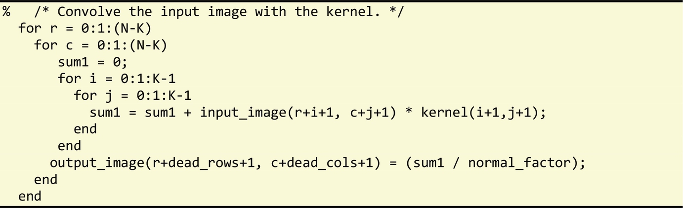
The edge detection application uses a function to convolve two input matrices. Fig. 3.2 presents an excerpt of a possible MATLAB code to implement the 2D convolution. In this example, the natively supported dot product “.⁎” is used to calculate the multiplications of the pixels in a window of K×K size with the kernel matrix. Fig. 3.3 shows a MATLAB code, very similar to the C code present in the repository, which does not use the “.⁎” operator.

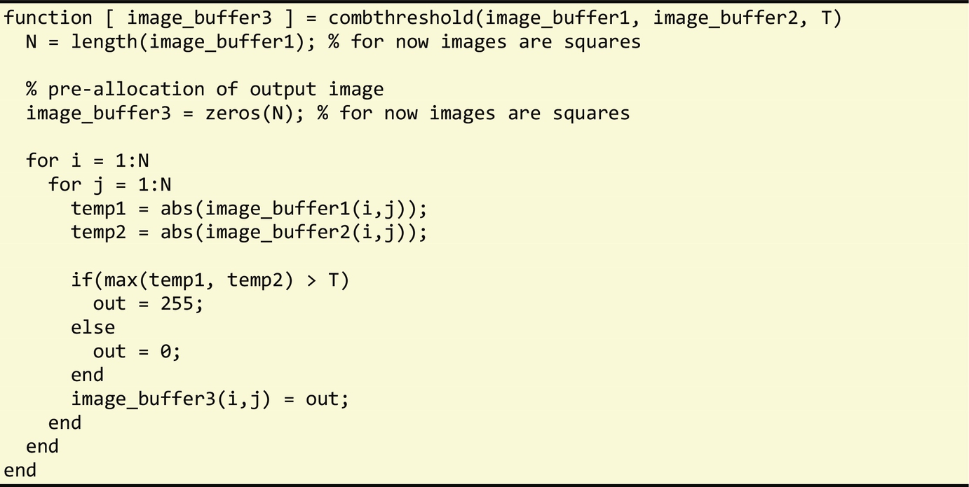
Other sections of the edge detection benchmark include (a) the merging of two images resulting from two convolutions that use different kernel values in a single image and (b) the generation of a B&W image (0 or 255 values) based on a threshold (T). Both computations are implemented in the combthreshold function shown in Fig. 3.4. The code for this function relies on MATLAB's ability to use matrices and to specify logical indexing. While this code version is very compact, it requires the use of temporary matrices to store intermediate results. The MATLAB statement max(abs(image_buffer1), abs(image_buffer2)) returns a matrix whose elements are the maximum values between the respective elements of abs(image_buffer1) and abs(image_buffer2). The result of max(abs(image_buffer1), abs(image_buffer2))>T provides a matrix of 1′s and 0′s indicating whether each element of the matrix max(abs(image_buffer1), abs(image_buffer2)) is larger than T or not.

Thus, in this example, four temporary matrices are used (including the two temporary matrices resultant from abs(image_buffer1) and abs(image_buffer2)). A translation pass from MATLAB to C would have to decide whether to use these temporary matrices, or instead decompose operations in a way that element-wise operations can be used, thus reducing memory use since the temporary matrices would not be needed. Fig. 3.5 presents another version of the combthreshold function, similar to the original C code, and Fig. 3.6 shows a MATLAB version obtained by a statement-by-statement translation from the original C code. These two versions make use of element-wise operations.

There are plenty of abstractions that may help to program applications and models. In addition to the inherent support for matrix operations as highlighted in this example, the support for regular expressions is another abstraction that provides enhanced semantic information in a compact form to a compiler. Recognizing a regular expression allows compilers to generate the most efficient implementation considering the target architecture, input data, and regular expression complexity. When direct support for regular expressions is not available, an implementation needs to be provided, which constrains the code transformations and optimizations of a compiler, and reduces opportunities for further transformations.
The use of higher abstraction levels allows the code to capture a specification rather than an implementation. As a specification, it focuses on the operations that need to be done (what), as opposed to the way they are done (how). As a result, code using low-level abstractions and close to a target implementation may make it difficult to identify alternative implementation paths. Domain-Specific Languages (DSLs) [8] allow the level of abstraction to be increased by providing domain-specific constructs and semantics to developers with which they can convey critical information that can be directly exploited by compilers in pursuit of optimized implementations for a given design.
The use of modeling languages and model-driven approaches has many benefits. Visual modeling languages such as Unified Modeling Languages (UMLs) [9] provide high abstraction levels and a specification of the application/system. They are, however, dependent on the capability of tools to generate efficient code and the availability of environments to simulate these models.
High levels of abstraction can also be provided by environments such as Simulink [2] and Ptolemy [10]. These can be seen as component-based simulation and development frameworks where visual languages (e.g., structuring a program in terms of components) are mixed with textual languages (e.g., to program the behavior of each component). These environments provide the capability to mix different components, such as parts of the computing system and emulator interfaces to these environments, while using models for each component. They also provide the possibility to describe each component with different levels of abstractions, e.g., using high- or low-level descriptions of the behavior, within the same framework. For instance, a system can be simulated such that one or more components use a high-level language description of the computation or can be simulated using a cycle-accurate model of a microprocessor. In some environments, one may simulate the system mixing models with “hardware in the loop” (i.e., using hardware for some of the components) [11].
Higher levels of abstraction can be provided in traditional textual languages such as C/C++ and Java using specific Application Programming Interfaces (APIs) and/or embedded DSLs [33]. An example of an API that provides high levels of abstraction is the regular expression APIs available for programming languages without native support for regular expressions (such as is the case of the Java language2).
3.2.2 Dealing With Different Concerns
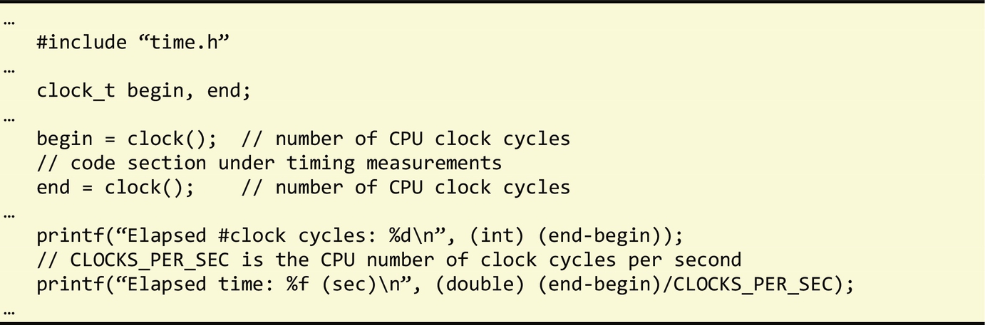
During the design cycle, developers may have to deal with different concerns that include emulating the input/output of the system, providing timing/energy/power measurements, and monitoring capabilities. These concerns might translate to specific code that must be introduced in the application, but ultimately removed in the final implementation and/or when deploying it to the target system. Timing and measuring the power and energy consumption of an application are examples of concerns typically considered during the design cycle. Figs. 3.7 and 3.8 present examples of code inserted in the application to provide such measurements. Both include calls to specific function libraries (APIs) to interface with hardware components (e.g., a timer and a power sensor).

The high abstraction level provided by programming languages such as MATLAB allows the specification of simulation models that take into account the connections to input/output components, but usually impose code to emulate certain features of the system. This code is in a later step removed from the application code. One example is the emulation interface to an input camera which loads images from files instead of connecting to a real camera. In some prototypes and production embedded implementations, these codes interface with a real camera.
It is common with programming languages such as C to use the preprocessor capabilities and the use of #ifdef and #define constructs to statically configure different versions of the application. This however pollutes the code and makes it difficult to maintain different versions, especially when dealing with many concerns that require many intrusive code changes. Figs. 3.9 and 3.10 present two examples of the use of #ifdef preprocessor directives to configure a section of an application according to the concern being addressed at a certain design point. The example in Fig. 3.9 shows C code and preprocessing directives that configure the way the input image is acquired: from a data file, from a memory mapped I/O, or defined by an initialization in a header file (“.h”). The options to read the image from a file or to define it as a “.h” file representing possible testing and evaluating scenarios are commonly defined before the deployment of the application to the target platform. In the example of Fig. 3.10, the preprocessing directives are used to configure the timing of the function using instrumentation (calls to functions of a timing library). Depending on how the library implements these functions, this example can even measure timing by using the hardware timers available in many microprocessors.


It is common to see preprocessing directives in most real-life C code, especially in the embedded programming domain. Developers use them to configure applications according to their particular needs. The selection of a particular configuration is done by changing the specific values or definitions directly in the source code or by using the support given by the compiler to control the preprocessor via command line options (e.g., GNU gcc supports the –D option to define values of #define preprocessor directives).
Preprocessing Directives
The C programming language has support for directives that are resolved during the preprocessing phasea (i.e., by a preprocessor) of the compilation. The preprocessor returns the source code to be input to the C compiler.
The set of directives include #include, #define, #ifdef, #else, #if, #elif, #ifndef, #undef, #error, etc. The directive #define can be used to define a constant or to define a macro. Following are two examples, one defining a constant and the other defining a macro to return the maximum of two values:

With GNU gcc, the result of the preprocessing phase can be output using the –E option (e.g., gcc –E file.c).
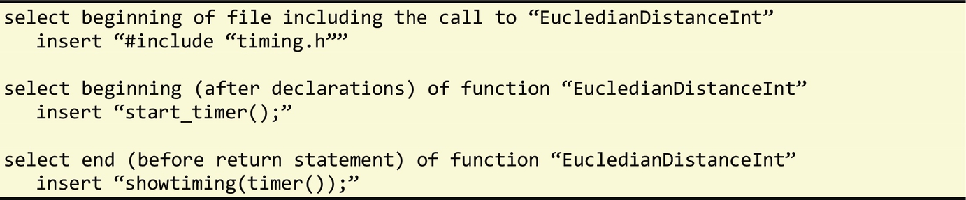
One possibility to help the global design/development cycle is to use an Aspect-Oriented Programming (AOP) approach [12,13] to provide the modularity level needed to configure the application and the different stages of the design/compilation flow (including different target languages), according to the requirements of each particular stage. The different code versions associated with a particular application concern can be programmed in separate modules called aspects, and a tool (known in the AOP community as weaver) is responsible to weave the application code with the aspects to automatically produce different code versions (e.g., one for modeling and simulation, one for prototyping, and multiple ones for implementation). Fig. 3.11 presents an AOP inspired example, considering the same configuration requirements of the first example that was previously presented to illustrate the use of #ifdef preprocessor directives (see Fig. 3.9). This example selects target elements of the program related to the concerns (such as the code to be timed) and specifies actions that include inserting target language code (in this case related to the use of a timing library). Although the application of this example is tied to a function named EucledianDistanceInt, the name of the function can actually be a parameter of the aspect shown in Fig. 3.11, making this aspect reusable for every function that needs to be timed via instrumentation.
3.2.3 Dealing With Generic Code
When developing a model using a high-level abstraction language, it is often desirable to reuse the model in various projects and applications. With this goal in mind, the code is developed in a more generic way, usually by providing certain options as parameters. This is common when programming for modularity and reusability. For instance, a function to sort a list of numbers is usually programmed to sort N numbers and not a specific number, e.g., 1000, that might be required for a particular application being developed. When considering MATLAB code, it is very common to develop code as generic as possible, taking into account various usage scenarios. This is also true in the context of the functions in the libraries that maximize reusability if provided with many usage scenarios in mind.
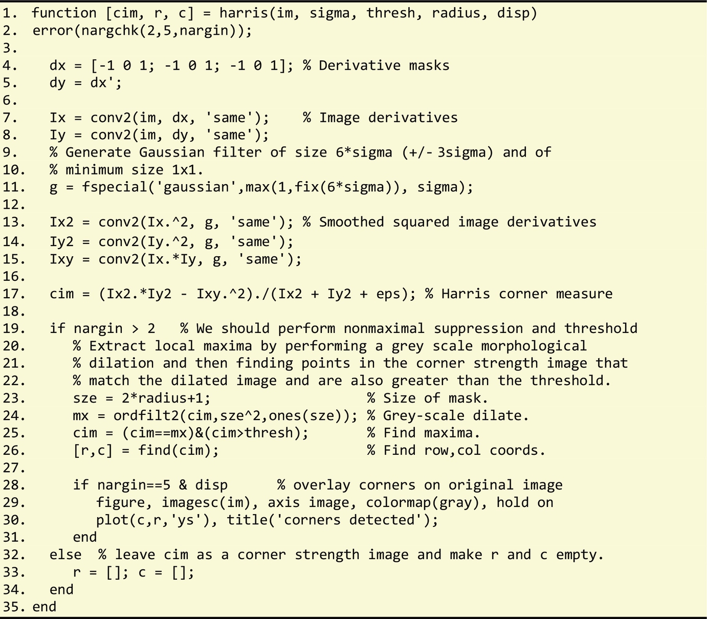
To illustrate this point, we present in Fig. 3.12 a MATLAB code of an image corner detector based on the Harris algorithm [14] widely used in vision-based navigation systems. Line 2 of this code checks if the number of arguments for each call of the function is between 2 and 5. If not, it reports an error. Since MATLAB functions can be called with a variable number of arguments, this kind of code, which checks the number of arguments, is very common (nargin is a system MATLAB variable with information about the arguments of the function). In line 19 there is once again a test to the number of arguments. If the function is not called with more than two arguments, r and c are returned empty (line 33), i.e., nothing is to be done and no corner is identified. This code is tangled with other nonfunctional concerns. For instance, lines 29–30 plot the resulting image and the corners. The function includes a parameter, disp, to control the plot.
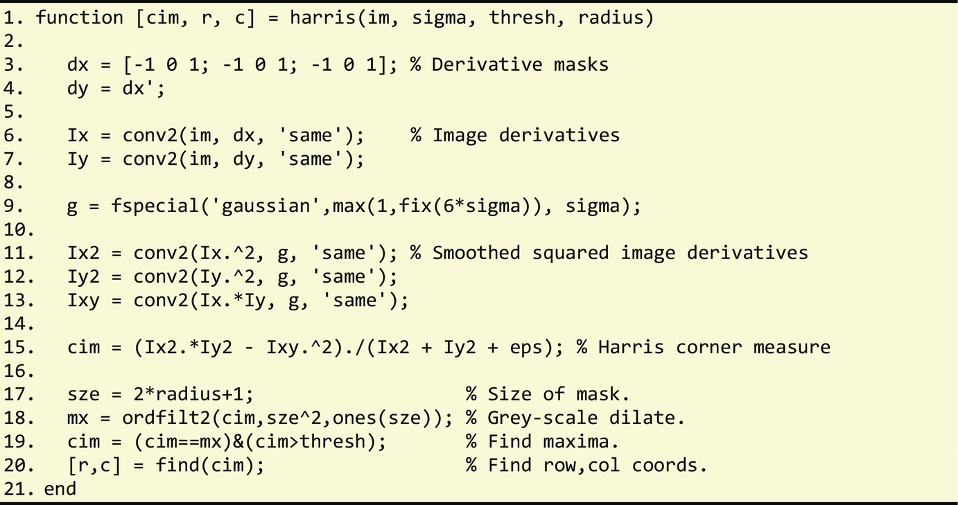
These two examples illustrate the inclusion of code that increases the usability of the function in a number of different scenarios/applications. Some of the included functionalities will hardly be present in the final system or product. Fig. 3.13 presents the code of the function without this additional code. The original function is now clearer as it only has the functionalities intended to be used in the final system.
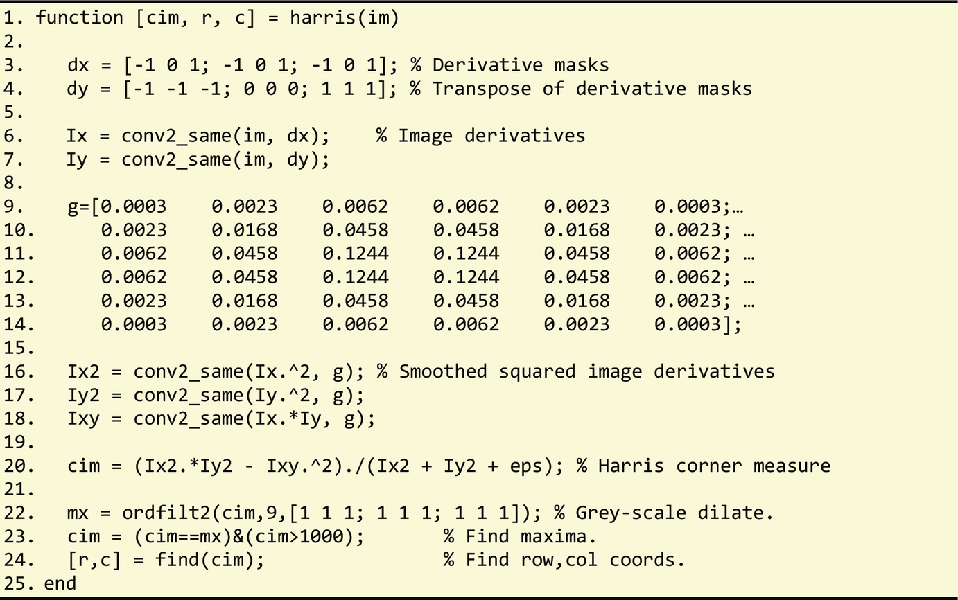
We note however that the code is still in a generic form, and with ample potential for performance improvement via specialization.3 Specifically, there are code sections that can be evaluated at compile time. For instance, dy=dx′; assigns to dy a matrix which is a transpose of the matrix of constants dx. Thus one possibility is to assign to dy the matrix of constants (i.e., dy=[-1 -1 -1; 0 0 0; 1 1 1]) instead of deriving it at runtime from dx. Another example consists on calculating g: g=fspecial('gaussian', max(1,fix(6⁎sigma)), sigma). It is common to call the algorithm with a specific value for sigma (1, 2, or 3) for a certain application. In each case, the statement on line 9 can be substituted by the assignment of the respective matrix of values according to the value of sigma. In a more generic implementation, but less generic than the one provided, one can substitute line 9 with one of the three matrices according to the value of sigma.
The code includes invocations to MATLAB functions provided by the MATLAB environment, such as conv2. Since conv2 is a library function, it is also a generic function providing the selection of the function code to be executed as its third parameter. In this case, all calls to conv2 in the code use ‘same’ as the third argument (in conv2(A, B, ‘same’)) and this means that conv2 returns the central part of the convolution of the same size as A. Thus, one can specialize a version of conv2 related to the ‘same’ case.
Fig. 3.14 shows a possible code version after specialization considering sigma and radius equal to one and thresh equal to 1000. Matrix g is now a matrix of constants and can even be moved inside function conv2_same thus enabling further optimizations in that function. The function ordfilt2 can be also specialized by moving the two arguments' constants inside the function.
As can be seen in this example, the potential for specialization when considering models and generic code can be very high. In Chapter 5, we describe code transformations that can be helpful for code specialization, e.g., in terms of performance and energy/power consumption.
3.2.4 Dealing With Multiple Targets
It is common to develop code that needs to be evaluated on different architectures in order to decide the target processing component to be used for each function or specific region of code, e.g., when targeting heterogeneous multicore architectures and/or architectures providing hardware accelerators, or when implementing products4 using different computing systems characteristics (e.g., when targeting different mobile devices).
The use of preprocessing directives is very common when developers need to have multiple implementations of certain regions of code, functions, constant values, options, etc. The options can be selected at the preprocessing stage and according to the target architecture. For instance, consider the example in Fig. 3.15, which measures the execution time of a region of code in a Personal Computer (PC) or in an embedded system. This example captures in the same source code: (1) the measurements of the execution time in a PC and (2) in an embedded system using a Xilinx MicroBlaze microprocessor implemented in an FPGA. In this example, depending on the definition (using #define) of “embedded_timing” or “pc_timing,” the preprocessor will select one of the code versions for measuring the execution time.

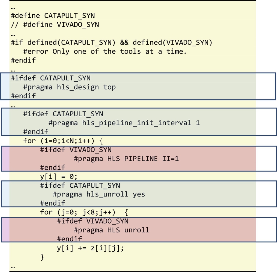
Even when a region of code is implemented using a particular hardware accelerator, different directives may have to be applied according to the toolchain used. Fig. 3.16 illustrates an example where a function is implemented on an FPGA-based hardware accelerator and different directives are used to instruct the target tool to convert the C function code into a custom hardware implementation. In this example, we consider Catapult-C (see, e.g., [15]) and Vivado HLS [16] as the target high-level synthesis (HLS) tools.
Similar examples can be provided when using different compilers (e.g., GCC, LLVM, ICC) or when using the same compiler but considering different target architectures.
Multitarget/Multitoolchains Using LARA
In the case of the LARA language, directives that are required in the code can be moved to LARA aspects, so that a weaver can inject the required code depending on the option provided by the user, as shown in the following example.

3.3 Translation, Compilation, and Synthesis Design flows
Given a high-level description of a computation to be mapped to a hybrid software/hardware execution platform, designers need to master a set of tools, namely:
• Compilers: These tools translate code described in a high-level imperative programming language, such as C, into assembly code targeting one or more cores, and using concurrency management primitives such as the ones offered by the OpenMP library (see Chapter 7). When interfacing with hardware or GPU devices, the code needs to include specific library and runtime environments for accessing the devices for data and computation synchronization.
• Synthesis tools: These tools translate a description in a hardware-centric language such as Verilog/VHDL, describing hardware behavior at Register-Transfer Level (RTL), to a target-specific representation suited for the mapping to, e.g., an FPGA device.
Fig. 3.17 depicts the general organization of the tools and the overall compilation and synthesis flow. At the core of this mapping process there is the need to interface the data and the control between the generated components, namely the software component where the control exists in a sequential or concurrent structure, and is defined by the semantics of the specific concurrency execution environment and the target hardware devices.
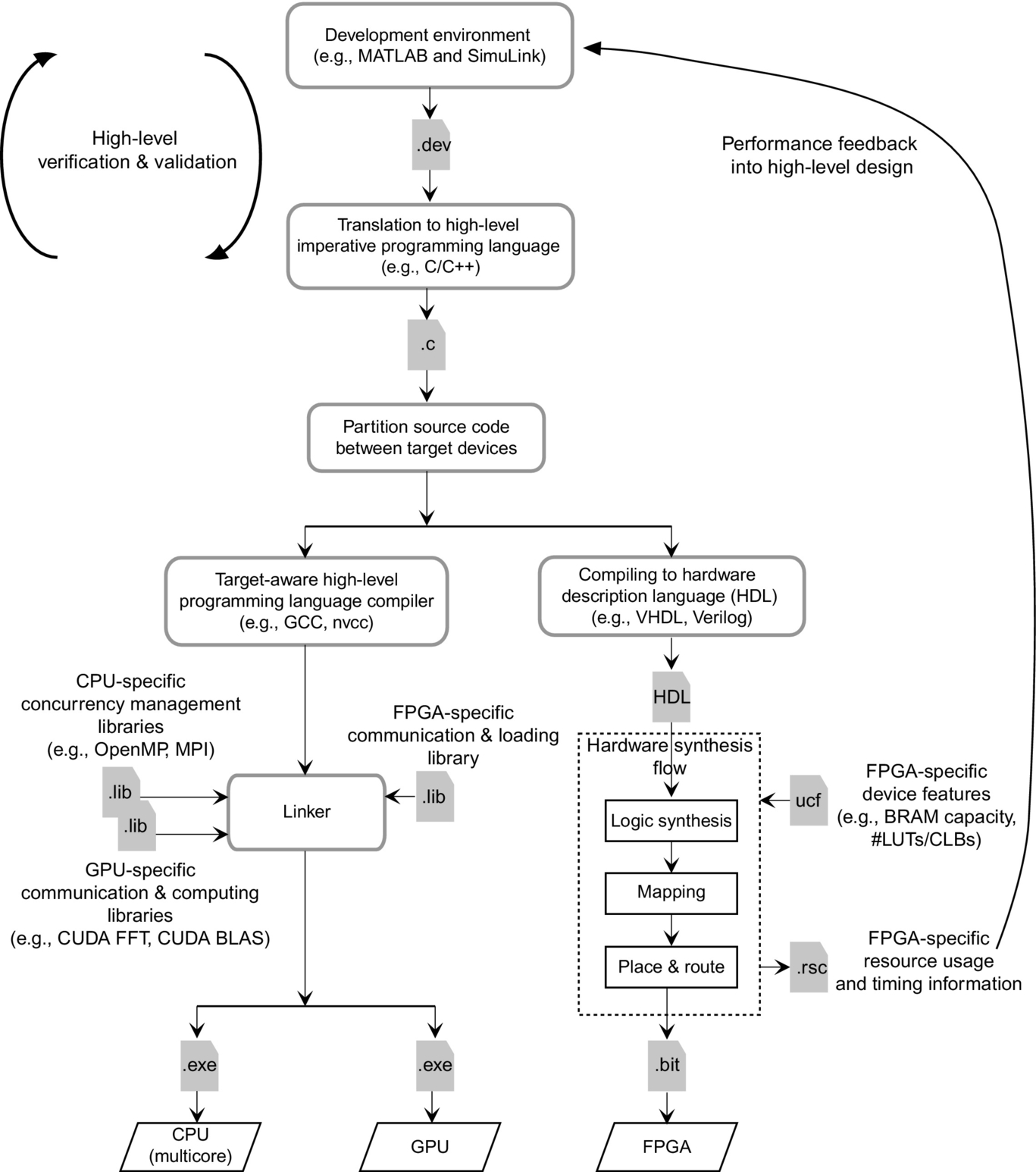
When targeting GPU devices, vendors offer libraries and interfacing environments that are still high level and map well to the abstractions of memory and control of traditional execution environments. Typically, the GPU interfaces have been structured around the abstraction of a coprocessor model, where input data is transferred to the device prior to execution followed by the corresponding transfer of results to the host processor address space. Vendors provide library functions to perform copy operations and provide compilers that translate high-level code to GPU assembly code. From a developer's perspective, the intellectual effort includes the encapsulation of which computation needs to be captured as a “kernel” and how to stage the data to and from the device to maximize performance. For many popular computations, such as Fast Fourier Transformations (FFTs) and linear Algebra functions, vendors even provide libraries that facilitate the access to highly tuned implementations of specific functions. Overall these approaches greatly simplify the reasoning of the program execution and hence the development and verification of concurrent codes.
Conversely, when targeting a hardware-centric device, such as an FPGA, there are significant differences in the compilation flow. While the data staging has been captured using the same approach of copying data to and from the device, the actual computation now requires the translation of the computation from a high-level programming language such as C to a hardware-oriented programming language such as Verilog or VHDL. Once the identification of the computation to be mapped to the device is done, the programmer must use a synthesis tool that will ultimately generate the programing binary file (a bitstream file, in the case of an FPGA device). The hardware design still needs to interface with a section of the FPGA that implements the data communication and synchronization protocols to be integrated with the execution of the host processor. In this context, and from the point of view of the host processor, the notion of a hardware thread has been exploited to facilitate not only the integration of the hardware devices but also its correct execution.
3.4 Hardware/Software Partitioning
An important task when targeting computing systems consisting of hardware and software components is hardware/software partitioning. Hardware/software partitioning is the process of mapping different sections of an application to distinct processing elements in a heterogeneous computing platform, such that performance and/or other nonfunctional requirements, e.g., energy consumption, can be met. A heterogeneous platform may harbor a diverse set of processing elements, such as general purpose processors (GPPs), FPGAs, and GPUs, and each of these devices may handle specific types of workloads more efficiently than others.
An efficient hardware/software partitioning process thus aims at distributing the workload among the most appropriate computation elements in a heterogeneous computing platform consisting of software and hardware components. This process can be considerably complex, as hardware platforms are becoming increasingly more specialized thus requiring enhanced programmer expertize to effectively exploit their built-in architectural features. Examples of heterogeneous hardware platforms include embedded systems consisting of Multiprocessor System-on-Chips (MPSoCs) provided by devices such as Zynq UltraScale+, the new Intel Xeon CPUs with integrated FPGAs, and emerging heterogeneous cloud platforms that offer on-demand computation resources.
The partitioning process identifies computations, described as sections of the application code, to be mapped to the different processing elements. The mapping process usually requires specific code generators and compiler optimizations for each target processing element. Once the mapping process is defined, the main application code needs to be modified to offload the computations and code sections to different processing elements. This offloading process, typically, involves the insertion of synchronization and data communication primitives. As each processing element may exhibit different energy/power/performance characteristics and the data communication between a host processor and the different processing elements may have different costs, the partitioning process must deal with a design exploration process with the goal of finding the best partitioning according to given requirements.
Given its importance, it is thus not surprising that there has been considerable research in hardware/software partitioning (see, e.g., [17]). The choice of techniques and algorithms depend on a number of factors, including:
• The number of candidate program partitions derived from an application description. We consider a partition to be a self-contained program module with well-defined inputs and outputs. Since each partition can be potentially executed on a different processing element, the mapping process needs to take into account the communication overhead between partitions when they are mapped on different processing elements. A partition can be defined by a program function or a subprogram module. However, a function may be further partitioned to find regions of code that are prime candidates for hardware acceleration, for instance, loop statements identified as hotspots in a program.
• The number of processing elements available for the mapping process, their corresponding architecture type, and interprocessor communication model. In particular, processing elements may communicate with each other by storing and accessing data through shared memory. Alternatively, in the case of heterogeneous architectures, each processing element may have its own local memory, and communication might be performed through shared memory and/or communication channels. In the case of non-existent shared memory, the mapping process becomes less flexible, with partitions that share the same data having to be possibly mapped to the same processing element.
In general, we can divide the hardware/software partitioning process in two broad categories: static and dynamic. The static partitioning process is determined at compile time and remains unchanged at runtime. In a dynamic partitioning process, the mapping is determined at runtime taking into account existing workload and device availability. In the remaining subsections, we describe design flows that support these two categories of hardware/software partitioning.
3.4.1 Static Partitioning
A typical design flow performing static partitioning is illustrated in Fig. 3.18 and consists of the following steps:
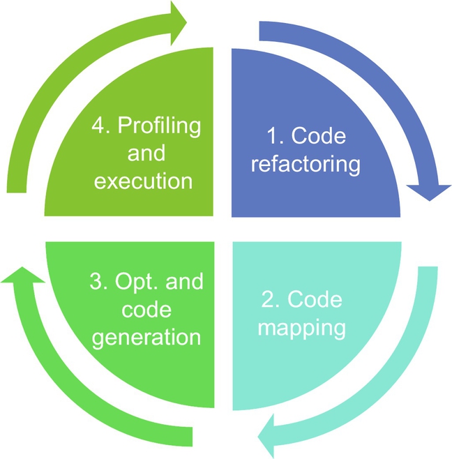
1. Refactoring the application to uncover candidate partitions. This involves merging and splitting functions from the original code to find a good set of partitions. Profiling can be performed to find hotspots and regions of code that may be accelerated, as well as to extract data communication patterns between different regions of code. Additional heuristics, based on source code inspection and profiling, can be applied to find partitions with minimized interdependences. Furthermore, partitions can be identified to uncover more opportunities for mapping a partition to different types of processing elements, thus increasing the chances of optimization.
2. Once a set of partitions is derived, the next problem consists in finding an efficient mapping. This usually involves employing a metaheuristic search algorithm, such as tabu search or simulated annealing, where the goal is to satisfy an overall nonfunctional performance goal. To achieve this, a cost model is required to estimate the performance of a particular mapping configuration, and guide the subsequent steps in the optimization process. This cost model may consider possible optimizations in the code for a particular processing element. For instance, loops can be pipelined to increase throughput if mapped onto an FPGA.
3. Once a mapping solution is found, the code may still be optimized to take into account the specific architecture of the processing element chosen. The optimization can be performed at source code level or at a lower intermediate representation (IR) level. Furthermore, as previously mentioned, the code is modified with synchronization and data communication primitives to offload computation between different processing elements. Once the final code is generated, it is compiled and linked by the different subtoolchains.
4. Finally, the generated application can be profiled on the target platform (or by simulation) to ensure it meets the application requirements. If not, then one can run the partitioning process from step 1. In this context, the synthesis and profiling reports are fed back to the refactoring (1), mapping (2), and optimization and code generation (3) steps to refine the hardware/software partitioning process.
The partitioning process also depends on the programming and execution models. Next we look at a typical example where a C application is mapped onto an heterogeneous embedded platform which hosts a CPU and an arbitrary number of hardware accelerators. We consider C functions to define partitions (note that other granularities may be used). Once the code is adequately refactored, a mapping process inspects the code and generates a static call graph G=(N, E), where nodes N represent function calls and edges E correspond to flow of data and control from one node to another. We consider that each function call instantiates a task. Because a single function can be invoked at different points in the program, two tasks can be instantiated from the same function and potentially mapped to different processing elements. Note that because a static call graph is generated at compile time it does not capture the number of tasks that are executed at runtime since this number may depend on runtime conditions, such as input data. Furthermore, in a call graph, edges can be associated with data flow information, such as the data type of input and output arguments.
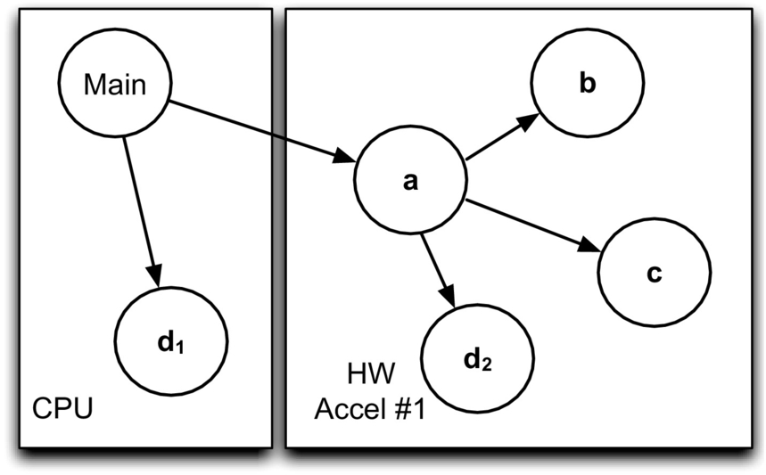
Consider the C program in Fig. 3.19A and the corresponding call graph presented in Fig. 3.19B. As can be seen, the main function invokes functions (tasks) a and d, and function a invokes functions (tasks) b, c and d. The invocations of function d in the call graph are identified as d1 and d2, respectively, as they correspond to two distinct invocation sites.

Once a call graph has been derived, the next step is to map it to the target heterogeneous architecture. We describe this mapping process for an illustrative heterogeneous embedded platform depicted in Fig. 3.20. This platform contains a CPU as the host processor and a set of hardware accelerators as coprocessors. Each processor has its own local memory with no global shared memory, hence communication is only allowed between the CPU and any of the accelerators. With this type of platform, the CPU runs the application with specific parts of the code (hotspots) offloaded to hardware accelerators to minimize overall execution time.

The task mapping process needs to find a configuration that minimizes the overall cost to meet a given performance goal:
where PEtask corresponds to the processing element onto each task of the application (App) is mapped for a particular configuration. The initial configuration, which serves as the baseline partitioning, places all tasks in the CPU. At each subsequent mapping step, the mapping algorithm tries to find a better mapping configuration by mapping one or more tasks from one processor to another, such that the overall cost is lower than the cost of the previous configuration. One challenge for the optimization process is to find a set of feasible mapping configurations, since not all configurations are valid. For instance, in our previous example, tasks a and b cannot be mapped to two distinct hardware accelerators, as in our target architecture, hardware accelerators cannot communicate directly with each other. For the same reason, if task b cannot be mapped to a hardware accelerator, then task a, which invokes task b, must also be mapped to the CPU. Hence, a search optimization algorithm, such as simulated annealing, can be associated with a constraint solver to find candidate mapping solutions. Also note that the cost estimation function must take into account not only the computation cost of migrating a task to a hardware accelerator, but also the communication overhead between the CPU and the hardware accelerator. Fig. 3.21 depicts a mapping solution for the previous example, where tasks a, b, c, and d2 are mapped to hardware accelerator #1 and the remaining tasks to the CPU.
3.4.2 Dynamic Partitioning
The underlying assumption of static hardware/software partitioning is that the mapping solution derived at compile time is resilient to changing runtime conditions. This may not be true for all classes of applications. Consider the AdPredictor machine learning algorithm [34] used to rank web execution for the Bing search engine, so that only ads with the highest probability of being clicked are presented. This algorithm's training phase takes as input ad impressions. Each ad impression captures the user session (IP, geographical location, search terms) and whether the corresponding ad was clicked or not. With each set of ad impressions, the training process updates a Bayesian model and improves its accuracy in ranking web ads.
Fig. 3.22 shows the performance of the training process using three implementations: a single-threaded CPU, a 20-threaded CPU, and an FPGA implementation. It can be seen from this figure that the most performant implementation depends on the job size, in this case, the number (volume) of ad impressions to be processed. The input size in this case matters because the FPGA design supports a deep streaming architecture which requires enough processing data to hide pipeline latency.

If the job size is only known at runtime, and the most efficient processing element depends on data size or other runtime conditions, then it may be preferable to perform the mapping process at runtime. One possible runtime management system is shown in Fig. 3.23. Here, the application explicitly invokes managed tasks, which are dispatched to the Executive process. This Executive process determines, based on several factors, which available processing element the task should be executed on.

As with static partitioning, dynamic partitioning relies on the cost estimation model to determine the most efficient processing element for a particular job. A cost model can be built offline by profiling implementations with different data inputs. Since it is unfeasible to profile all combinations of inputs, an estimation model can be derived through regression and further improved by monitoring the application during execution.
One implication of the dynamic partitioning process is that all the application code, except for managed tasks, is handled by the host CPU. A managed task, however, is handled by the Executive process, and its execution depends on available task implementations and computing resources. In particular, a task can be associated to multiple implementations each of which can be executed on a specific type of processing element. Hence, if a heterogeneous computing platform includes N homogeneous processing elements, then in the presence of an implementation of that type, there is a choice of N processing elements it can be executed on. In this context, a central repository or library will store (at runtime) metadata associated with each implementation and accessed by the Executive process to make a mapping decision at runtime, in particular:
• Implementation characterization. Each implementation must be associated with metadata information, which includes preconditions and performance models. Preconditions allow the Executive process to filter out implementations unsuited to run a particular task, for instance, a hardware sorting implementation that only supports integer numbers up to 256. Preconditions can be expressed as a set of predicates, which must all evaluate to true to be considered for execution. A performance model allows the Executive process to estimate the baseline performance of an implementation when executing a task given a set of input attributes, such as data size and data type. In Fig. 3.24 we can see that if an incoming task has a volume of 100 ad impressions, then the Executive process may choose the multithreaded CPU implementation and thus avoiding to offload the computation onto a hardware accelerator, whereas a task with 100 thousand impressions would in principle execute faster on an FPGA.

• Resource availability. A performance model might not be enough to estimate the fastest processing element given a particular task. For instance, the fastest executor (as identified by using a performance model) may be busy and is only able to execute a task at a later stage, thus executing slower than a potential earlier executor. Hence, to select the most efficient processing element, the Executive also needs to estimate how long a task will wait until it is actually executed. This is done by inspecting the size of the device queue associated to each processing element and the cost of each task execution currently in the queue. Once an implementation and a processing element are chosen, they are pushed into the corresponding device queue (see Fig. 3.24).
Recent research in this area has led to the development of several dynamic mapping approaches targeting heterogeneous platforms, including StarPU [35], OmpSs [18], MERGE [36], SHEPARD [37], and Elastic Framework [19]. These approaches offer similar runtime mapping mechanisms with differences on the programming and execution models used, how implementations and computing resources are characterized, the target platforms supported, as well as scheduling strategies to optimize workload distribution. For instance, OmpSs supports explicit annotations of task dependences in the source code, allowing the runtime management system to execute tasks asynchronously (and potentially in parallel) while satisfying their dependences.
3.5 LARA: a language for Specifying Strategies
LARA [21, 38] is an AOP language [22, 39] specially designed to allow developers to describe: (1) sophisticated code instrumentation schemes (e.g., for customized profiling); (2) advanced selection of critical code sections for hardware acceleration; (3) mapping strategies including conditional decisions based on hardware/software resources; (4) sophisticated strategies determining sequences of compiler optimizations, and (5) strategies targeting multicore architectures. Furthermore, LARA also provides mechanisms for controlling tools of a toolchain in a consistent and systematic way, using a unified programming interface (see, e.g., [20]).
LARA allows developers to capture nonfunctional requirements from applications in a structured way, leveraging high/low-level actions and flexible toolchain interfaces. Developers can thus benefit from retaining the original application source code while exploiting the benefits of an automatic approach for various domain- and target component-specific compilation/synthesis tools. Specifically, the LARA AOP approach has been designed to help developers reach efficient implementations with low programming effort. The experiences of using aspects for software/hardware transformations [23] have revealed the benefits of AOP in application code development, including program portability across architectures and tools, and productivity improvement for developers. Moreover, with the increasing costs of software development and maintenance, as well as verification and validation, these facets of application code development will continue to be of paramount significance to the overall software development cycles.
In essence, LARA uses AOP mechanisms to offer in a unified framework: (a) a vehicle for conveying application-specific requirements that cannot otherwise be specified in the original programming language, (b) using these requirements to guide the application of transformations and mapping choices, thus facilitating DSE, and (c) interfacing in an extensible fashion the various compilation/synthesis components of the toolchain.
LARA support is provided by a LARA interpreter and weavers. Examples of tools using the LARA technology are the following four compilers5: MATISSE (a MATLAB to C compiler), Harmonic (a source-to-source C compiler), MANET (a source-to-source C compiler), ReflectC (a CoSy-based C compiler), and KADABRA (a source-to-source Java compiler).
We briefly present in this section the main constructs of the LARA language and how it can be used to modify the code of a given application to meet certain requirements.
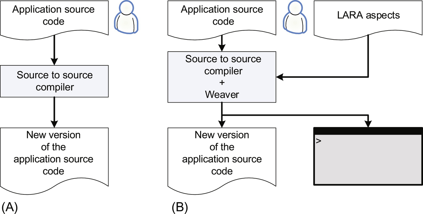
The LARA code is modular and organized around the concept of aspects. Aspect definitions can invoke other aspects, and thus, a set of LARA aspects can be applied to a given input program. A special tool, called a weaver, executes these aspects and weaves the input program files according to the actions expressed in the aspects to produce new files. Fig. 3.25 shows the inputs/outputs of two kinds of source-to-source compilers. The first (Fig. 3.25A) which is common, considers the control via directives and/or command line options. The second (Fig. 3.25B) is extended to support LARA. In this case, the output console shown is mainly used to print the messages from LARA aspects (e.g., via LARA println statements). We note that other uses of LARA can include the control of a compiler in the context of machine code generation.
3.5.1 Select and Apply
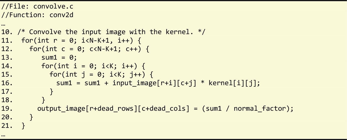
An important feature of LARA is its ability to query program elements using a method similar to database queries. Fig. 3.26 shows a simple example of a select construct for querying loops in the input source code. The elements of the program queried by a LARA select statement are named join points, and a list of supported join points is defined for each target programming language. One can select a specific program element in the code according to its position (e.g., in terms of nested structure) in the code. For instance, we are able to select a specific loop in a specific function for a given file. The loop word used in this example refers to the loop join point in all programming languages currently supported by LARA. If this select is applied to the C code presented in Fig. 3.27, the result is a list of the 4 loops in the code. Each LARA join point includes a set of attributes which are associated to properties of a specific program element. For instance, some of the attributes associated to the loop join point are is_innermost, is_outermost, line, and type. We can use the attributes to verify certain characteristics of the associated program element. For instance, select loop{type==“for”} end selects only loops of type for in the code.

Once the program elements have been selected, we can also apply actions to each of them. For this, the LARA language provides the apply statement. Usually, each select has an associated apply section. The apply section supports JavaScript code mixed with specific LARA constructs. Fig. 3.28 shows an example where for each loop in the code the weaver prints to the console the type of each loop found. To access information about the program element, the join point can be used in the apply section by prefixing its name with $ ($loop in the example shown). In order to access an attribute of a specific join point, the name of the attribute prefixed by “$” must be followed by “.” and by the name of the attribute (e.g., $loop.type). When the aspect is applied to the code in Fig. 3.27, the output is as follows:
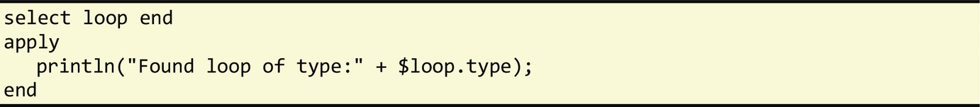
  Found loop of type: for
  Found loop of type: for
  Found loop of type: for
  Found loop of type: for
If the println statement is replaced by println(“Is innermost? ”+$loop.is_innermost); the result is as follows:
  Is innermost? false
  Is innermost? false
  Is innermost? false
  Is innermost? true
The semantics of a select-apply section resembles that of a query language. For each program element found by the select statement, the corresponding code of the apply section is executed. In the example shown in Fig. 3.28, the code does not modify the program but outputs messages to the console. This is an important mechanism to report program characteristics determined by a static inspection and/or analysis of the input program.
The select-apply constructs are required to be part of an aspect module. Each aspect module begins with the LARA keyword aspectdef followed by the name of the aspect and ends with the keyword end. Fig. 3.29 shows an example of a LARA aspect that reports properties for each loop found in the code. We note that in this example the select continues to query for loops but in this case we expose the chain of join points file.function.loop to access attributes of file (e.g., $file.name) and function (e.g., $function.name), besides the ones related to the loops (e.g., $loop.type, $loop.num_iterations, $loop.rank, $loop.is_innermost, $loop.is_outermost).

When the aspect in Fig. 3.29 is applied to the code of Fig. 3.27 when N and K are equal to 512 and 3, respectively, it yields the output as follows:
  Found loop:
             File name: convolution.c
             Function: conv2
             Loop line number: 11
             Loop type: for
             Loop number of iterations: 510
             …
             Is innermost? false
             Is outermost? true
  …
  Found loop:
             File name: convolution.c
             Function: conv2
             Loop line number:15
             Loop type: for
             Loop number of iterations: 3
             …
             Is innermost? true
             Is outermost? false
We can also use variables in LARA aspects. They can be global to the aspect or local to each apply section. Fig. 3.30 presents the use of a global aspect variable to count the number of for-type loops in a program.
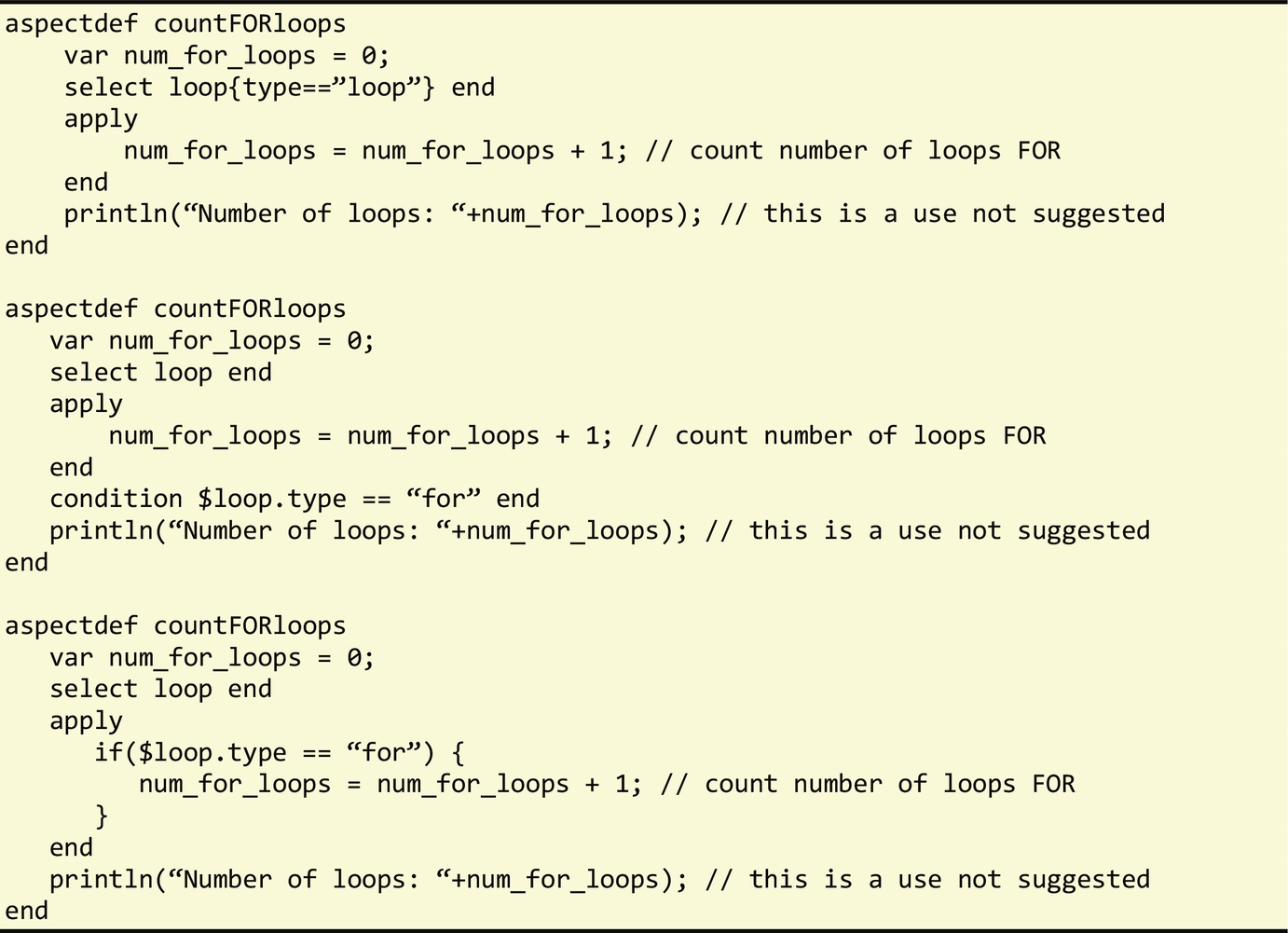
In addition to the ability to query loops of a certain type using the select statement (e.g., select loop{type==“for”} end), LARA also supports the condition statement which filters the join points that are processed in the apply section. Conditions can be expressed using complex Boolean expressions, while select filters only allow Boolean comparison of an attribute against an expression. Another possibility is to use if statements in the apply section. Fig. 3.30 shows three cases of LARA code, which produce the same results.
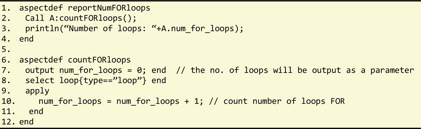
Each LARA aspect module definition can have multiple select-apply statements and these behave using a declarative semantic. More specifically, the aspect statements are executed in sequence as they occur in the LARA file. It is thus the responsibility of programmers to ensure that dependences are satisfied by placing the aspect statements in the right order. As can be observed in the aspect example in Fig. 3.30, this sequential evaluation leads to the correct reporting of the number of loops (println statement in the end of the aspects). An alternative aspect specification (yielding the same outcome) would use a second aspect to invoke the aspect that counts the number of loops and to print its value at the end of its execution (see Fig. 3.31). Note that the code within each apply section is strictly imperative.
In the presence of multiple aspect definitions in the same file, the first aspect definition is considered the main aspect and will be automatically executed first. Other aspects are only executed if they are explicitly invoked either directly or indirectly by the main aspect's execution.
The list of attributes, actions, and join point children associated to a specific join point can be queried with the following attributes: attributes, actions, and selects, respectively. For instance, $loop.attributes outputs the list of attributes (their names to be more precise) for the join point loop, $loop.actions reports the weaver actions related to the join point $loop, and Weaver.actions outputs the weaver actions available to LARA.
3.5.2 Insert Action
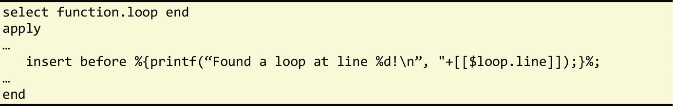
LARA provides an insert action to inject code in the application's source code. This action can be mixed with other statements in the apply section. The code to be inserted is identified by the delimiters %{ and }% or ‘ and ’, where the former captures multilined code, and the latter captures single-lined code (similar to a string). The insertion of the code can be performed before, after, or replace the associated join point. Fig. 3.32 shows a simple example that inserts a printf statement before each loop in the source code. By default, the insert is associated to the join point of the last element of the select expression (in a chain), but one can explicitly identify the associated join point by prefixing the insert with join point followed by “.”. For instance, $loop.insert would be equivalent to the insert in Fig. 3.32.

It is possible to pass data of the aspect and/or join points to the code to be inserted. Fig. 3.33 presents an extension of the previous example to indicate the number of the source-code line of each loop found. In this case, the line attribute of the join point loop ($loop.line) is passed to the inserted code as a parameter between [[]]. The weaving process will substitute, for each execution of the insert statement, [[$loop.line]] by its actual value. In a similar way one can use LARA variables in the sections of code to be inserted.
Insert actions provide a powerful mechanism to add/replace code in an application. The possibility to specify strategies for the insertion of the code is one of the most useful LARA concepts. Fig. 3.34 shows an example of a LARA aspect which specifies the insertion of calls to function QueryPerformanceCounter6 for measuring the time execution of applications, written in the C programming language, when running in the Windows operating system. Note that the aspect needs to insert the #include (line 5), the declaration of the variables to be used (lines 10 and 11), and the insertion of the code to initialize and start the measurements (select-apply in line 14) and to end the measurements and to output the result (select-apply in line 24). This aspect provides an automatic scheme to modify an application with a timing concern similar to the one presented in Fig. 3.7 and using calls to the clock() function.7 The code presented in Fig. 3.34 can be easily modified to provide a timing strategy using clock().

3.5.3 Exec and Def Actions
In the previous section, we presented the insert action and showed how to program strategies for instrumenting code in the source code of an application. LARA provides other types of actions. Two actions used to modify the application by using specific code transformations supported by the compiler used are exec and def. The exec action is used to execute weaver-defined actions, such as specific compiler passes (e.g., loop unrolling). The def action is used to modify certain application artifacts such as data types of variables.
Fig. 3.35 presents the use of the exec action (line 6) to unroll loops. In this case, the aspect specifies to unroll by a factor, denoted by variable “factor,” loops that are innermost and of type for. When applied to the source code of an application, this aspect will unroll all the loops respecting these conditions. Fig. 3.36 presents a more elaborated aspect which prevents the full unrolling of innermost loops when the unrolling factor is zero and the selected loop has a large number of iterations, in this case more than eight iterations.

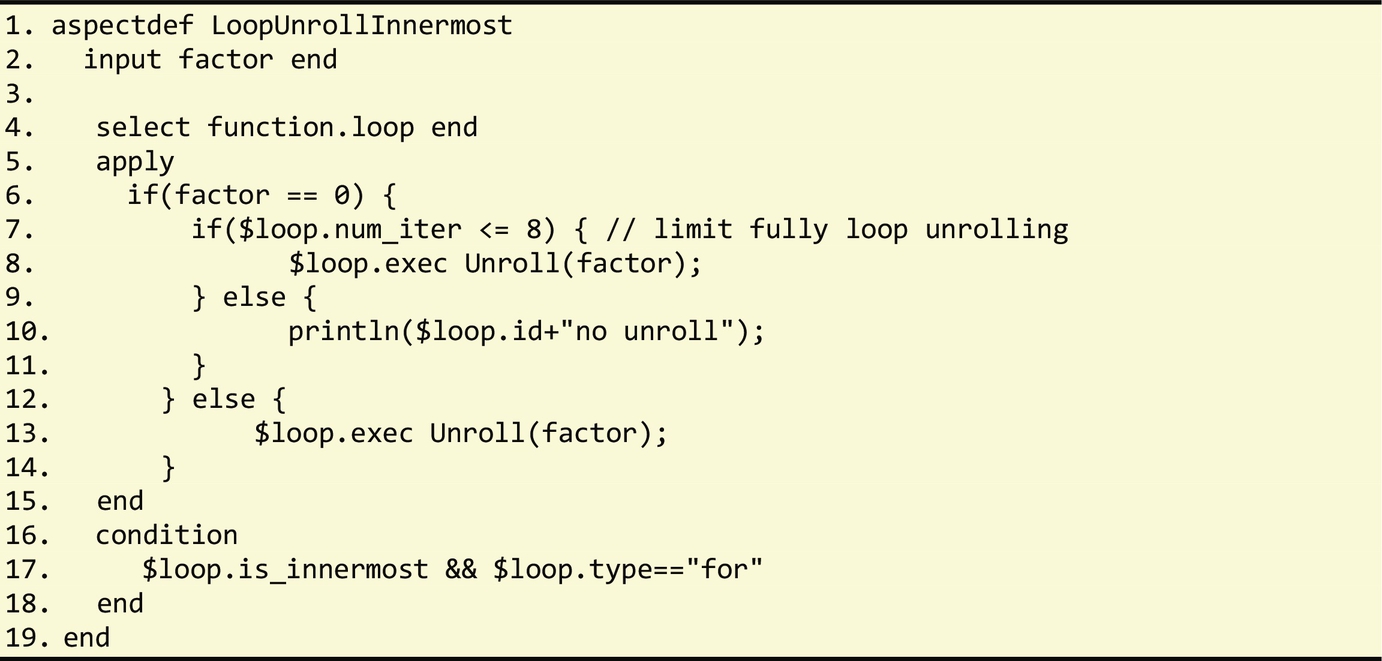
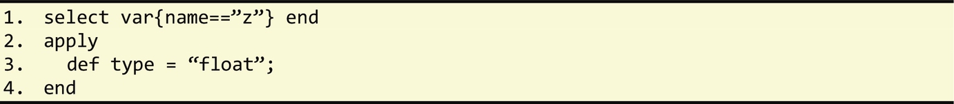
Fig. 3.37 presents an example where the variable z is assigned to type float. This example uses the def action and implies changes in the Intermediate Representation (IR) of the compiler.
3.5.4 Invoking Aspects
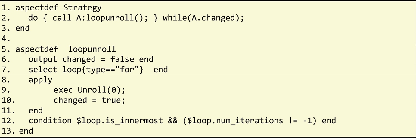
LARA provides a mechanism for invoking an aspect from an aspect definition and optionally share data between them through its input and output parameters. This enhances modularity and reuse. Fig. 3.38 shows a simple example where one of the LoopUnrollInnermostaspects presented before is invoked with 2 as its argument.

When calling an aspect with output parameters, the only way to access the output values is through the assignment of an identifier to the call and then to use a syntax similar to a field access. For instance, in call A:countFORloops(); in line 2 of Fig. 3.31, the identifier A is used to represent that specific call of aspectcountFORloops. The use of A.num_for_loops in line 3 allows the value of num_for_loops to be accessed in that specific call.
The current semantics related to calls varies in terms of insert and exec/def actions. The result of the insert actions is not made available to subsequent weaving statements until the output code is generated and input to the compiler. That is, the code modifications using insert actions are not immediately visible during the weaving process responsible for those insertions.
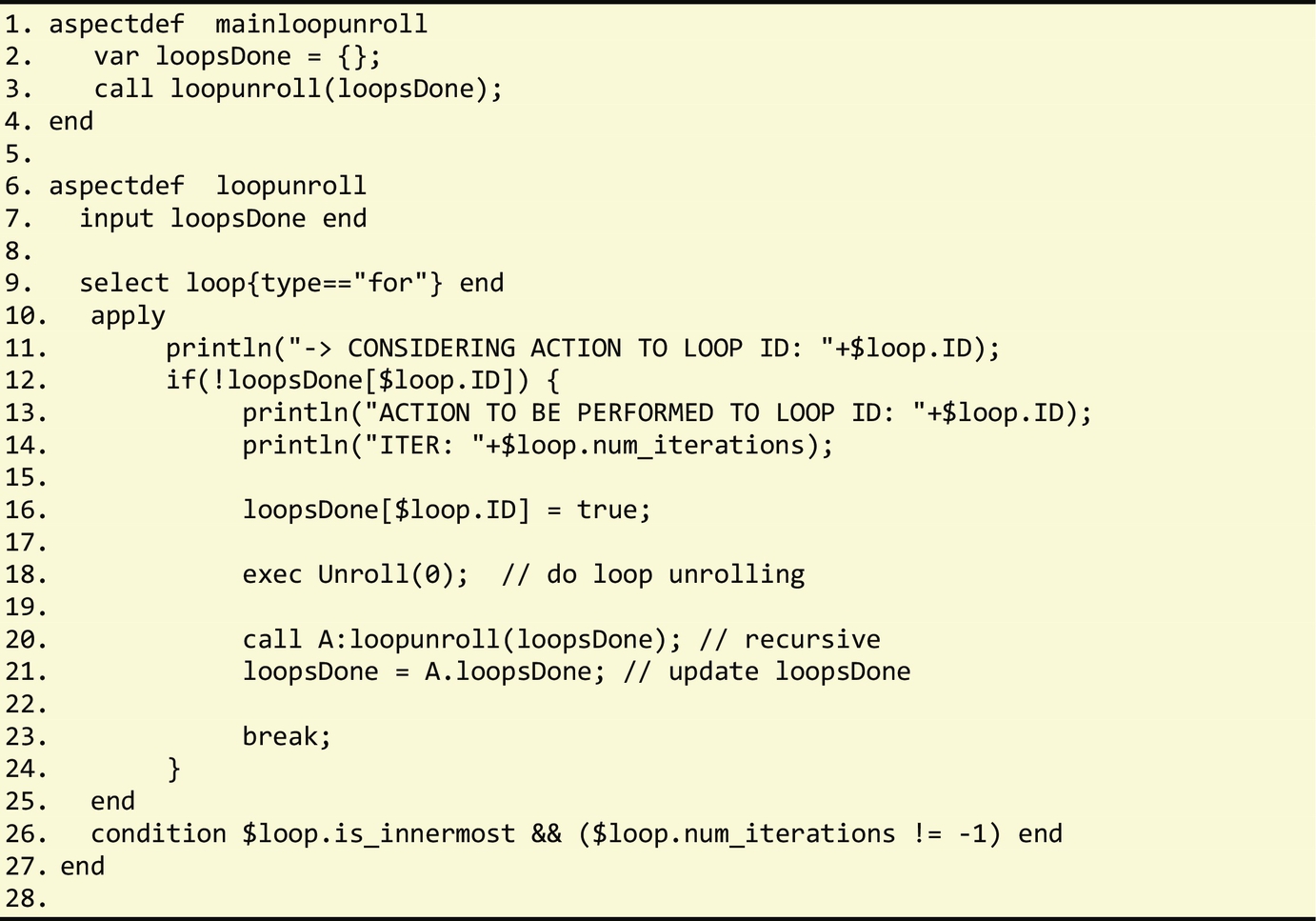
On the other hand, the changes that result from the exec/def actions are available once execution enters a new aspect. We show here an example of what the semantic of the exec/def actions implies. The aspect presented before in Fig. 3.35 unrolls the innermost for loops. If we apply the aspect with a factor=0, we will fully unroll all the loops that fit a specific condition. This aspect does not fully unroll the loops recursively because it only considers the original innermost loops found in the application. The recursive invocation of this aspect would lead to the full unrolling of all the loops regardless of their original position in the nested loop structure. Fig. 3.39 presents a possible aspect that recursively unrolls all loops in the program. Note the use of the break instruction in line 23 to prevent the unrolling of loops that no longer exist as a result of having been fully unrolled. Fig. 3.40 illustrates an aspect with the same goal but using iteration instead of recursion.
3.5.5 Executing External Tools
LARA also allows to explicitly invoke external tools from aspects and to import data output from the execution of such tools, providing a transparent way to use the feedback information to make decisions at the LARA level and iterations over a specific tool flow.
Fig. 3.41 presents an example which invokes Xilinx backend tools having as input a VHDL or Verilog description of the hardware to be synthesized, mapped, placed, and routed to a specific target FPGA. The LARA aspect also provides support for the execution of one or more tools based on the value of the opt input parameter. The @function used in the println statements in lines 6, 11, 15, and 19 is the data output from the execution tool represented as a JSON object.

The execution of the xst tool (line 3 of the LARA aspect) will provide the following attributes and the correspondent values according to the input VHDL/Verilog code and target FPGA:
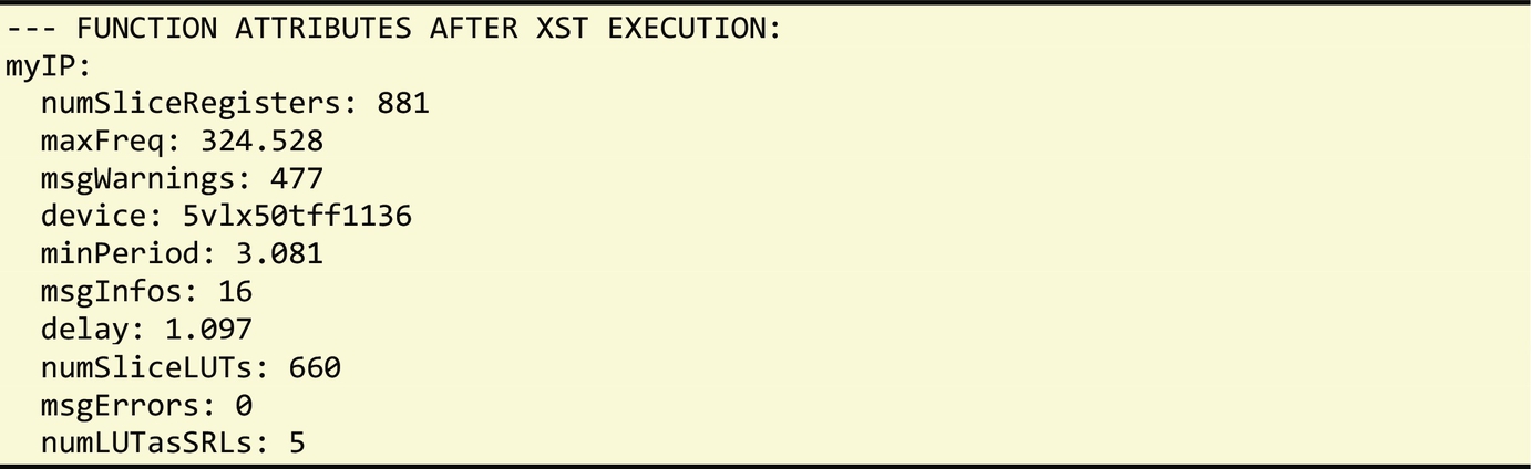
Fig. 3.42 presents another LARA aspect that includes a call to the aspect shown in Fig. 3.41, to a High-Level Synthesis (HLS) tool to generate the VHDL description from an input C function and to a VHDL simulator. The aspect is responsible for reporting the results regarding clock cycles and execution time considering the maximum clock frequency reported by the tools.

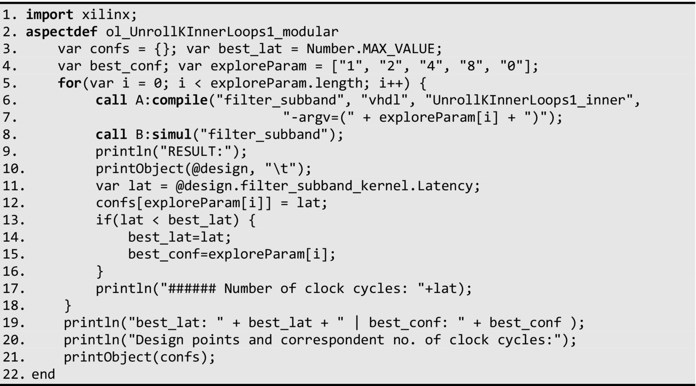
This support provided by LARA to execute tools (including ones aided with LARA) conveys developers with artifacts and with a unified view which diminishes the efforts to program and evaluate DSE schemes. Fig. 3.43 shows a simple example of a DSE scheme. In this case, four different loop unrolling factors and no loop unrolling are explored with the goal of achieving a hardware design with the lowest possible latency.
3.5.6 Compilation and Synthesis Strategies in LARA
The compilation and synthesis strategies in LARA include code transformations, exploration of parameters, and specification of complementary program knowledge that can be conveyed to other compilation tools in producing better quality code. As mentioned in Chapter 1, the use of LARA in this book intends to fulfill two goals: (1) to provide a specification of code transformations and optimization strategies and (2) as a DSL to be used in experiments regarding learning activities. Goal (2) has focused on using specific tools with LARA support, namely, the following tools:
• MANET, a source-to-source C compiler based on Cetus: http://specs.fe.up.pt/tools/manet/
• KADABRA, a source-to-source Java compiler based on Spoon: http://specs.fe.up.pt/tools/kadabra/
• MATISSE, a MATLAB to C/OpenCL compiler: http://specs.fe.up.pt/tools/matisse/
The LARA strategies used in the context of goal (2) have been developed partially based on the support that third-party tools provide to implement the semantics of the LARA actions. It is conceivable that LARA strategies, while well defined, cannot be used in cooperation with tools that do not export a “control interface” that allows the LARA aspects to carry out the corresponding actions.
3.6 Summary
This chapter presented the main concepts regarding the first stages of an application's design cycle such as its specification, prototyping and development with the main emphasis on the abstraction levels, and on how to deal with different concerns; the specializations required when dealing with generic code and with high-level models, and on how to deal with multiple targets. This chapter also introduced the concepts of translation, compilation, and synthesis design flows, and hardware/software partitioning (including the mapping of computations to heterogeneous architectures). Lastly, we have described an AOP language, LARA, specially designed to allow developers to describe sophisticated code instrumentation schemes and advanced mapping and compilation strategies.
3.7 Further Reading
Design flows operating on heterogeneous platforms with hardware accelerators have been the focus of recent research (see, e.g., the hArtes design flow in [24]). One of the main tasks of a design flow involves the decision to map computations into software and/or hardware components. This task is traditionally known as hardware/software partitioning (see, e.g., [25]), especially when the target system considers software components implemented in CPUs and hardware components synthesized from the input computations. More complete forms of hardware/software partitioning also consider hardware accelerators being then synthesized and/or existent as coprocessors. Recently, the migration of computations from the CPU to hardware accelerators (including GPUs and FPGAs) is referred as offloading computations to these devices.
Hardware/software partitioning started with static approaches, i.e., with partitioning performed at design/compile time [26, 40]. At compile time there have been approaches starting with the computations described in high-level code (such as from C/C++ code) or with the binaries and/or traces of executed instructions [41]. Approaches addressing dynamic hardware/software partitioning have been focused more recently (see, e.g., [27,42]). Other approaches consider the static preparation of hardware/software components, but delegate to runtime the decision to execute computations in hardware or software. For instance, Beisel et al. [28] present a system for deciding at runtime between hardware/software partitions at library function level. The system intercepts library calls and for each call it decides to offload the call to a hardware accelerator. The decision is based on tables storing information about the execution time for each supported function and for different data sizes. Additional decisions can also consider other information, such as the number of iterations (calculated at runtime) each loop will execute for each execution point, to decide offloading computations to hardware accelerators. Vaz et al. [29] propose to move the decision point within the application to possibly hide some overheads, such as the preparation of the coprocessor execution.
Current heterogeneous multicore architectures support GPUs and/or reconfigurable hardware (e.g., provided by FPGAs) with the possibility to provide different execution models and architectures, thus increasing the complexity of mapping computations to the target components. Systems may have to consider not only code transformations that might be suitable for a particular target, but also decide where to execute the computations, which is not trivial. For instance, when considering a target architecture consisting of a CPU+GPU, a system may need to decide about the execution of OpenCL kernels in a multicore CPU or in a GPU [30]. The complexity of the problem and the variable parameters involved to make a decision are being addressed by sophisticated solutions, such as the ones using machine learning techniques to estimate execution time based on static and dynamic code features [31]. Other authors address the data migration problem when targeting GPU acceleration [32]. As these are hot research topics, it is expected that further solutions will be proposed especially considering the interplay between code transformations, workloads, runtime adaptivity, and the specificities of the target architecture.