7.1 Introduction

High-level languages, such as C and C++, are designed to allow code to be portable across different types of computation platforms, in contrast to assembly language in which the level of abstraction is close to the machine code instruction set. Compilers are responsible for translating such high-level descriptions into efficient instructions, allowing application code to be mostly oblivious to the underlying architecture. This approach worked well during the single-core era, in which CPU-based processors became incrementally more powerful by successive increases in clock frequencies and by the introduction of specialized instruction sets that could be automatically exploited by compilers with little or no effort from developers. However, due to the physical limits concerning heat dissipation and gate delays, CPU speeds ceased to increase. This stagnation gave way to more complex platforms that: (a) embraced native hardware support for parallel execution with more independent processing cores; (b) became more heterogeneous to support specialized and customized computation; and (c) became more distributed to support applications requiring large-scale computations, including Big Data and HPC. However, this considerable increase in computation capacity came at a cost: the burden of optimization shifted from compilers back to developers.

In this chapter, we expand on the topic of code retargeting introduced in Chapter 6, covering techniques geared toward specialized computing devices (GPUs and FPGAs) and heterogeneous platforms in general. Code retargeting is the process of optimizing the application source code to run more efficiently on a particular platform architecture. The most basic computation platform corresponds to a single type of computing device, such as a general-purpose processor (e.g., a multicore CPU) or a hardware accelerator (e.g., FPGAs and GPUs). We can build a more complex and heterogeneous computing platform by combining general-purpose processors with hardware accelerators. Applications targeting these heterogeneous platforms run on general-purpose processors and offload critical parts of their computation to hardware accelerators.

The structure of this chapter is as follows. In Section 7.2, we cover the roofline model and explain how it can guide the code retargeting process. In Section 7.3, we focus on the problem of workload distribution, which deals with how computations can be effectively offloaded to hardware accelerators in a heterogeneous platform. Section 7.4 covers the OpenCL framework for targeting CPU platforms with GPU accelerators, and Section 7.5 focuses on the high-level synthesis (HLS) process for translating C programs into FPGA hardware designs. Section 7.6 presents two LARA strategies assisting HLS. The remaining sections conclude this chapter and provide further reading on the topics presented in this chapter.

7.2 Roofline Model Revisited

When retargeting an application to a complex heterogeneous platform, it is important to understand the main characteristics of the application's workload, as well as the features of the target architecture.

We begin with the workload characterization. The way we characterize workloads depends largely on the type of application we are targeting. For instance, for floating-point applications it is relevant to count the number of floating-point operations. We can extend this workload characterization by also counting the number of bytes transferred between the memory and the processor when executing load and store operations. In general, the application workload is proportional to the problem size: a large problem, such as a 1000×1000 matrix multiplication, leads to a larger workload than a 100×100 matrix multiplication since the former computation requires a larger number of operations and bytes transferred.

We now assume a simple platform consisting of one compute node and one memory unit. To estimate the time required to execute a given workload, defined as (#operations, #bytes moved), we need two pieces of information about the platform: the computational throughput (how many operations the compute node can process per second) and memory bandwidth (the rate at which data is read from or stored to memory).

It is important to note that the computational throughput is often not a constant but rather a function of the size of data processed. This is true, for instance, when computer architectures have deep processing pipelines, requiring them to be filled to attain maximum throughput. However, the most prevalent factor preventing peak performance is that the rate at which the compute node processes data is dependent on the rate at which it can access data. In other words, if the data access rate is lower than the computation throughput then bandwidth becomes a performance bottleneck.

This implies that the workload distribution needs to account not only the computation throughput for each of the platform compute nodes, but also data movements, in terms of data size and data access rate, as these factors directly affect performance. For this reason, it is useful to consider another metric to characterize and compare workloads: operational intensity, which is the ratio of total number of operations to the total data movement (bytes): $\frac{\#\mathit{operations}}{\#\mathit{bytes}\mathit{moved}}\mathrm{Flops}/\mathrm{byte}$. For instance, FFTs typically perform at around 2 Flops/byte, while N-body simulation performs in the order of tens of Flops/byte. Intuitively, algorithms requiring more cycles dedicated to data operations (loads and stores) than computation operations will typically exhibit lower computational intensity and be more likely to be memory bound. Conversely, algorithms requiring more computation than data movement will have a higher computational intensity and be more likely to be compute bound.

The roofline performance model [1,2], introduced in Chapter 2, provides a useful visualization of how a given application (or one of its kernels) performs when exploiting various architectural and runtime features of a specific platform (e.g., multicore, hardware accelerators, cache memories). The most basic roofline model can be derived by plotting the computational throughput (y-axis) as a function of operational intensity (x-axis). The resultant curve, as presented in Fig. 7.1, defines two performance bounds under which the application performance exists: the memory bandwidth ceiling and the computation performance ceiling, both of which are platform specific. As expected, implementations with high operational intensity will hit the peak computation ceiling as they require more computation than data movement, otherwise they will hit the memory bandwidth ceiling.

When retargeting an application or a kernel to a specific platform, we seek implementations that perform as close as possible to the peak computation performance of the platform. In the example presented in Fig. 7.1, only implementation Z hits this ceiling. While it may not always be possible to achieve peak computation performance, especially in cases where an algorithm has inherently low computational demands, the following techniques can be used to maximize performance:

• Data locality. Given that modern-day platforms contain several types of memory storage units, with different sizes, speeds, and access models (shared or distributed), it is important to improve data locality, such that compute units can access data as fast as they can process them. This means making effective use of multilevel cache systems (Section 6.7) and using local device memories to store intermediate results for hardware accelerators working as coprocessors. Other techniques to improve data locality include software data prefetching, which are used to mitigate the long latency of memory accesses either from main storage or from upper levels of the cache hierarchy and thus reduce the stall cycles in the execution pipeline of modern processors. The basic idea behind prefetching is to load data in advance to hide the latency of memory accesses, hence making data already available when the computation needs it. If the hardware supports prefetching instructions and buffers, compilers can exploit them by judiciously placing prefetching instructions in the code. When data locality is not optimized, there is a risk of increasing the amount of data movement (e.g., due to cache misses or having superfluous transfers between CPU and hardware accelerators), which leads to lower operational intensity and designs becoming memory (or I/O) bound, as is the case of implementation X shown in Fig. 7.1.

• Heterogeneous computation. General-purpose processors are flexible enough to execute most workloads. However, this flexibility comes at the price of having a relatively low performance ceiling. Consequently, even implementations with a lower computational intensity may quickly hit the platform's performance ceiling (see dashed line on implementation Y shown in Fig. 7.1). To further increase the height of the performance ceiling, developers need to exploit the platform's specialized features. The key idea is to map a given workload (or selected parts of this workload) to specialized processing units, including: (i) packing scalar instructions into vector instructions to perform more operations in parallel (Section 6.4); (ii) running a kernel in parallel over multiple data points on a GPU (Section 7.4); (iii) streaming data across a customized pipelined data path architecture on an FPGA (Section 7.5). Such mapping requires a deep understanding of the architectural features of the compute devices (CPU, GPU, FPGA) and the type of workload amenable to run on such devices. This effort allows the peak performance to increase, typically between 1 and 2 orders of magnitude, over a general-purpose processor.

• Multicore and multiprocessors. With today's platforms consisting of multicore CPU machines with computation capacities that can be extended by connecting several machines together with fast network interconnects, there is the potential to run very large computationally intensive workloads. Such workloads can be partitioned within the cores and processors of each machine (Section 6.5) and across available machines (Section 6.6), such that each compute unit operates at its peak computational throughput. The process of partitioning and mapping workload can be done statically if all parameters (e.g., workload type and size) are known at compile time, or otherwise decided dynamically by the platform's runtime system.

7.3 Workload Distribution

As discussed in the previous section, it is important to understand both the nature of the application and the features of the underlying platform to derive an efficient mapping between them. This is particularly critical, as platforms are becoming more heterogeneous, allowing various types of hardware accelerators to assist in speeding up computations running on the host processor. Hence, we need to understand in what conditions should we offload computations to these devices and what factors affect overall performance. This is the subject of this section.

When computations are offloaded to an accelerator, there is a cost overhead that is absent when the entire computation is carried out by the host processor, namely:

1. Data transfer to and from the host to the accelerator's storage or address space.

2. Synchronization to initiate and terminate the computation by the accelerator.

Given the current system-level organization of most computing systems, data needs to be physically copied between storage devices often via a bus. This has been traditionally the major source of overhead when dealing with accelerators. Furthermore, the host needs to actively engage in polling to observe the termination of the computations on the accelerators, thus synchronization also incurs an overhead, which is typically proportional to the number of tasks to be offloaded to the accelerators.

Hence, in cases where the host and the accelerators execute in sequence (i.e., the host blocks until the accelerator terminates execution), it is only profitable to offload kernels to accelerators if they exhibit a very high operational intensity (the ratio of computation to data used—see previous section). Furthermore, for offloading to be profitable, the accelerator needs to execute the computation considerably faster than the host to offset the aforementioned overheads.

To measure the benefits of offloading, we need to first select one or more metrics of performance, such as execution time and energy consumption. Typically, developers compare the execution time of a kernel running on the host for each relevant problem of size n, i.e., T_comp^host(n), against the time it takes to perform the same computation using an accelerator, say T_comp^accel(n).

Note that the execution time (or another metric such as energy) can depend nonlinearly on the problem size. For linear algebra operations, such as matrix-matrix multiplications, simple algorithms can be described as having a computational complexity that increases with the cube of the input matrix dimension size n (the number of columns or rows for squared matrices), i.e., the computation time on the host can be modeled as $T_{\mathrm{comp}}^{\mathrm{host}}\left(n\right)={\alpha }_0{n}^3+{\beta }_0$ for a square matrix with dimension size n. For other computations, the complexity might be quadratic as in $T_{\mathrm{comp}}^{\mathrm{host}}\left(n\right)={\alpha }_0{n}^2+{\beta }_0$. When the same computation is executed on an accelerator, while the complexity may not change, the values of the coefficients α₀ and β₀ may be different due to other sources of overhead, namely, data transfer cost.

To assess the benefits and hence to aid in deciding whether to offload computations, programmers can build execution models for the host and for the accelerator, capturing both execution time and any additional overheads for a given problem size. As an example, consider the following two execution models:

1. Blocking coprocessor execution model. In this execution model, the host processor is responsible for transferring data to and from the accelerator storage space (or simply copying it to a selected region of its own address space) and by initiating and observing the completion of a task's execution by the accelerator. While the host processor can carry on other unrelated computations as the accelerator is computing, it is often the responsibility of the host to check when the accelerator has terminated its execution. The following analytical expression (Eq. 7.1) captures the execution time of this model:

$T_{\mathrm{comp}}^{\mathrm{accel}}\left(n\right)=T_{\mathrm{comm}}^{\mathrm{host}2\mathrm{accel}}\left(n\right)+T_{\mathrm{exec}}^{\mathrm{accel}}\left(n\right)+T_{\mathrm{comm}}^{\mathrm{accel}2\mathrm{host}}\left(n\right)$

Clearly, for an accelerator operating under this execution model to be effective, the data transfer time needs to be either reduced to a minimum or hidden as is the case of the nonblocking model as explained next.

2. Nonblocking coprocessor execution model. In this execution model, and after triggering the execution of the first task on the accelerator, the host can initiate a second task (if is independent from the previous one) by transferring the data for the second task to the accelerator while the accelerator is carrying out the computation corresponding to the first task.
The analytical expression in (Eq. 7.2) captures the execution time of this model for a “steady state” operation mode, where the communication for the first and the last task is ignored, and where the max function is used to capture the fact that if the computation takes longer than the communication, the accelerator will delay the communication or if the data transfer from the host to the accelerator takes longer than the computation of the previous task, the accelerator will stall.

$T_{\mathrm{comp}}^{\mathrm{accel}}\left(n\right)=max\left(T_{\mathrm{comm}}^{\mathrm{host}2\mathrm{accel}}\left(n\right)+T_{\mathrm{comm}}^{\mathrm{accel}2\mathrm{host}}\left(n\right),T_{\mathrm{exec}}^{\mathrm{accel}}\left(n\right)\right)$

This model is only possible if there are no dependences between the two computations and there is enough memory space to save the data for the computation scheduled to be executed next. This execution model reaches its maximum benefit when the communication between the host and the accelerator can be entirely masked by the computation, and excluding the initial and final computations, the execution time is simply dictated by the maximum duration of the communication or the accelerator execution.

Given the execution models described earlier, and under the assumption developers can accurately model the various sources of overhead, it is possible to determine when it is profitable to use an accelerator to execute a set of computational tasks based on the problem (workload) size n. For simplicity, we assume the overall computation is composed of a series of tasks with the same data sizes.

Using the execution models earlier, we can depict in a chart when it becomes profitable to offload the computation's execution to an accelerator with the two execution models. Fig. 7.2 illustrates when it is profitable to offload the computation to an accelerator in both execution models described earlier. In this illustrative example, we have assumed a quadratic cost model with respect to the input problem (or data) size for the computation effort of the host processor and the accelerator for any of the tasks involved. In contrast, the communication costs for the transfer of data to and from the accelerator follow a linear cost model.

This figure depicts two breakeven points beyond which, and despite the communication overhead of the data transfer, it becomes profitable to use the accelerator for offloading computation. Clearly, the relative position of these breakpoints depends on the relative values of the fixed overhead costs, δ, and the α and β coefficients for the various model components outlined in Eqs. (7.1) and (7.2).

The performance speedup for either of these two execution models is thus given by the expression in Eq. (7.3), which can asymptotically reach the raw performance benefit of an accelerator when the overhead of communication and synchronization reaches zero.

$\mathrm{SpeedUp}=\frac{T_{\mathrm{comp}}^{\mathrm{host}}}{T_{\mathrm{comp}}^{\mathrm{accel}}}=\frac{T_{\mathrm{exec}}^{\mathrm{host}}}{T_{\mathrm{exec}}^{\mathrm{accel}}}$

Note that while it may be profitable to offload the computation to an accelerator, the problem size might become too large to fit the accelerator's internal storage. In this scenario, developers need to restructure computations by resorting to different partitioning strategies so that the data for each task considered for offloading can fit in the accelerator's storage.

The communication cost between the host and the accelerator is modeled using a simple affine function as illustrated in Fig. 7.3, where n corresponds to the problem size (Eq. 7.4), which is proportional to the amount of data transferred. Note that other application parameters can be considered when modeling communication cost. For instance, for image processing, the amount of data transferred might depend not only on the image size, but also on the color depth used and filter size.

$T_{\mathrm{comm}}^{\mathrm{host}2\mathrm{accel}}=\beta n+\delta$

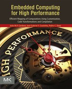
Commonly, developers resort to analytical modeling based on empirical data to model the performance of specific tasks on their accelerators. Often, this approach uses regression models to fit the observed data to an assumed analytical model (see Fig. 7.4). With these execution models, and knowing the problem size and reasonable estimates of the execution on the accelerators, developers can determine when it becomes profitable to offload computations to the accelerators. The analysis described here, although using a simple sequential execution model, can be extended (arguably not in a trivial fashion) to an execution system with multiple accelerators by adjusting the various coefficients of the communication and synchronization costs.

7.4 Graphics Processing Units

A Graphics Processing Unit (GPU)¹ is a specialized type of hardware accelerator originally designed to perform graphics processing tasks. However, with the advent of programmable shaders and floating-point support, GPUs were found to be considerably faster than CPUs for solving specific types of problems, such as scientific applications, that can be formulated as uniform streaming processes. This type of processes exploits data parallelism, applying the same kernel (operation) over a large sequence of data elements.

One popular approach for programming GPUs is OpenCL [3,4], an open standard which is currently maintained by the consortium Khronos Group. Unlike CUDA, OpenCL is vendor independent and supports a wide range of compute devices spanning from multicore CPUs to FPGAs. In this section, we consider the use of OpenCL to program GPUs in the context of a heterogeneous platform where a CPU acts as the host and one or more hardware accelerators (GPU) act as coprocessors. In this type of platform, applications running on the host are sped up by offloading sections of the program to the GPUs. The choice of which parts of the program are offloaded to the GPU, and indeed to any hardware accelerator acting as a coprocessor, is critical to maximize overall performance.

As mentioned in the beginning of this section, data-parallel algorithms are a good fit for GPU acceleration, since the GPU architecture contains hundreds of lightweight processing units able to operate over several data items in parallel. Moreover, algorithms must be computationally intensive to maximize the utilization of the GPU compute resources and in this way, hide memory latency. This is because GPUs support fast context switching: when memory accesses are required while processing a subset of data elements, this subset is put on hold, and another subset is activated to keep the GPU compute resources busy at all times. Additionally, problems requiring streaming large sequences of data are also a good fit, as they reduce the data movement overhead between the host and the GPU memories.

To express data parallelism in OpenCL, programmers must specify the global dimensions of their problem. The global dimensions specify the total problem size, describing an array of data elements processed using the same operation, known as a kernel. Global dimensions can be expressed in 1D, 2D, or 3D spaces depending on the algorithm. In this context, a work-item is an instance of the kernel that executes on one data element of the array defined in the global dimensions' space, thus being analogous to a CPU thread. Therefore the global dimensions define the number of work-items that will execute on the hardware device. Consider, for instance, the following problems:

1. 1D: process an 8k audio sample using one thread per sample: ~8 thousand work-items

2. 2D: process a 4k frame (3840×2160) using one thread per pixel: ~8 million work-items

3. 3D: perform raytracing using a voxel volume of 256×256×256: ~16 million work-items

Current GPU devices are not big enough to run 16 million work-items at once, hence these items are scheduled according to available computing resources. Still, the developer is responsible for defining explicitly the total number of work-items and its dimensions according to the problem at hand. For instance, the developer can decide to process a 4k frame by using a work-item that operates on a line instead of a pixel, thus requiring a total of 2160 work-items instead of around 8 million. This affects not only the number of work-items that need to be scheduled but also the granularity of each work-item.

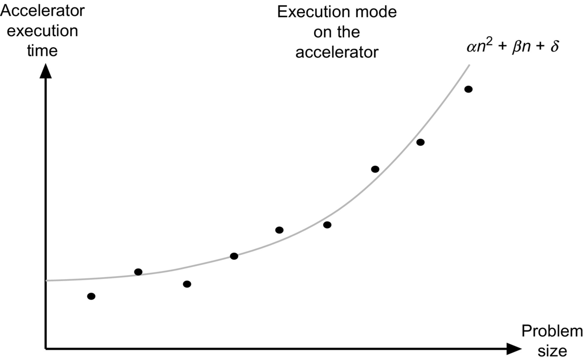
Developers must also specify the local dimensions of their problem, which defines the number of work-items executing together in a work-group. The size of this work-group must evenly divide the global size in each dimension. Hence, if the global dimensions of a problem are 1024×1024, then 512×512 and 128×128 are valid local dimensions, but 512×100 is not valid as 100 does not evenly divide 1024. The work-groups are, thus, important as they define the set of work-items logically executed together on a physical compute unit, and it is only within the context of a work-group that work-items can be synchronized. In other words, if synchronization is required between work-items, then they need to be confined within the same work-group (see Fig. 7.5).

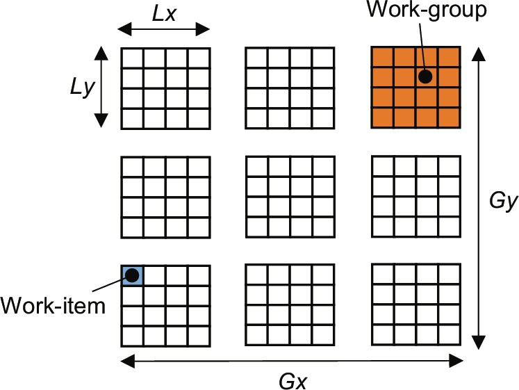
A kernel is a unit of code executed in parallel at each point of the problem domain and developers express data-parallel computations by writing OpenCL kernels. OpenCL kernels are described using the C99 language syntax, although they exhibit significant differences with respect to its software (CPU) counterpart. One common way to convert a regular CPU program to OpenCL kernels is to inspect the loops in the program and attempt to convert innermost loop statements as an operation applied at each point of the loop iteration space. We now consider the following C loop which performs element-wise multiplication of two vectors:

This code can be translated to an OpenCL kernel as follows:

In this example, the kernel corresponds to the innermost loop body, which is executed n times, where n is the specified number of work-items defined by the global dimensions (in this example operating in an 1D space). The get_global_id routine returns the identifier of the work-item, so that it knows which data it is meant to work on.

Regarding the kernel description, OpenCL provides a few extensions to the standard C99 language, namely:

• Vector data types and operations. Vector data types are defined by the type name (char, uchar, ushort, int, uint, float, long, and ulong) followed by a literal value n which corresponds to the number of elements in the vector. These data types work with standard C operators, such as +, -, and *. The use of vectors in an OpenCL kernel is automatically compiled to exploit SIMD units if the hardware supports it, or to regular scalar code if not.

• Rounding and conversion routines. As in C99, implicit conversions are supported for compatible scalar data types, whereas explicit conversions are required for incompatible scalar types through casting. OpenCL extends this support for both scalars and vectors with a set of explicit conversion routines with the form: convert_<destination_type>(source), as shown in the following example:

In addition, OpenCL supports a set of rounding routines with the syntax convert_<destination_type>[_sat][_rounding_mode](source), where the optional sat mode specifies saturation for out-of-range values to the maximum possible value the destination type can support. There is support for four rounding modes, namely: rte (round to the nearest even), rtp (round toward positive infinity), rtz (round toward zero), and rtn (round toward negative infinity). If no modifier is specified, it defaults to rtz for integer values and rte for floating point values.

• Intrinsic functions. OpenCL supports a number of math library functions with guaranteed accuracy, e.g., exp, log, sin, fmax, and modf. OpenCL also supports two additional sets of fast intrinsics versions, which provide a trade-off between precision and performance, in the form of native_<fn> (fastest but no accuracy guarantee) and half_<fn> (less performant than the corresponding native intrinsic but with higher accuracy), e.g., native_log and half_log. The use of intrinsics guarantees availability (all OpenCL compliant devices are meant to support them), thus increasing the portability of OpenCL code across heterogeneous devices.

In addition, OpenCL includes utility functions that provide information about each work-item, allowing the kernel to identify which operation to perform and on which data:

• Global dimensions: (1) get_global_id(dim): returns a unique global work-item ID for a particular dimension; (2) get_work_dim(): returns the number of global dimensions; (3) get_global_size(dim): returns the maximum number of global work-items in a particular dimension.

• Local dimensions: (1) get_local_id(dim): returns a unique work-item ID for a particular dimension within its work-group; (2) get_local_size(dim): returns the number of local work-items in particular dimension; (3) get_num_groups(dim): returns the number of work-groups that will execute a kernel for a particular dimension; (4) get_group_id(dim): returns a unique global work-group ID for a particular dimension.

We now focus on the OpenCL runtime architecture introduced in Chapter 2. At the top level, OpenCL exposes a set of platforms (see Fig. 7.6) each of which is composed by a set of computing devices supplied by the same vendor, such as AMD, Intel, and Nvidia. There are many types of OpenCL devices, including CPUs, GPUs, and FPGAs. Each device has a global memory with a specific size and bandwidth. Typically, GPUs have faster memories than CPUs as they can support higher computational throughputs. Devices can communicate with each other (e.g., via PCIe), but typically devices within the same platform can communicate more efficiently with each other. Each device is composed of a set of compute units which operate independently from each other, and each compute unit has a set of processing elements. All OpenCL devices exhibit this architecture organization, varying in the number of compute units, the number of processing elements, and their computational throughput capacity.

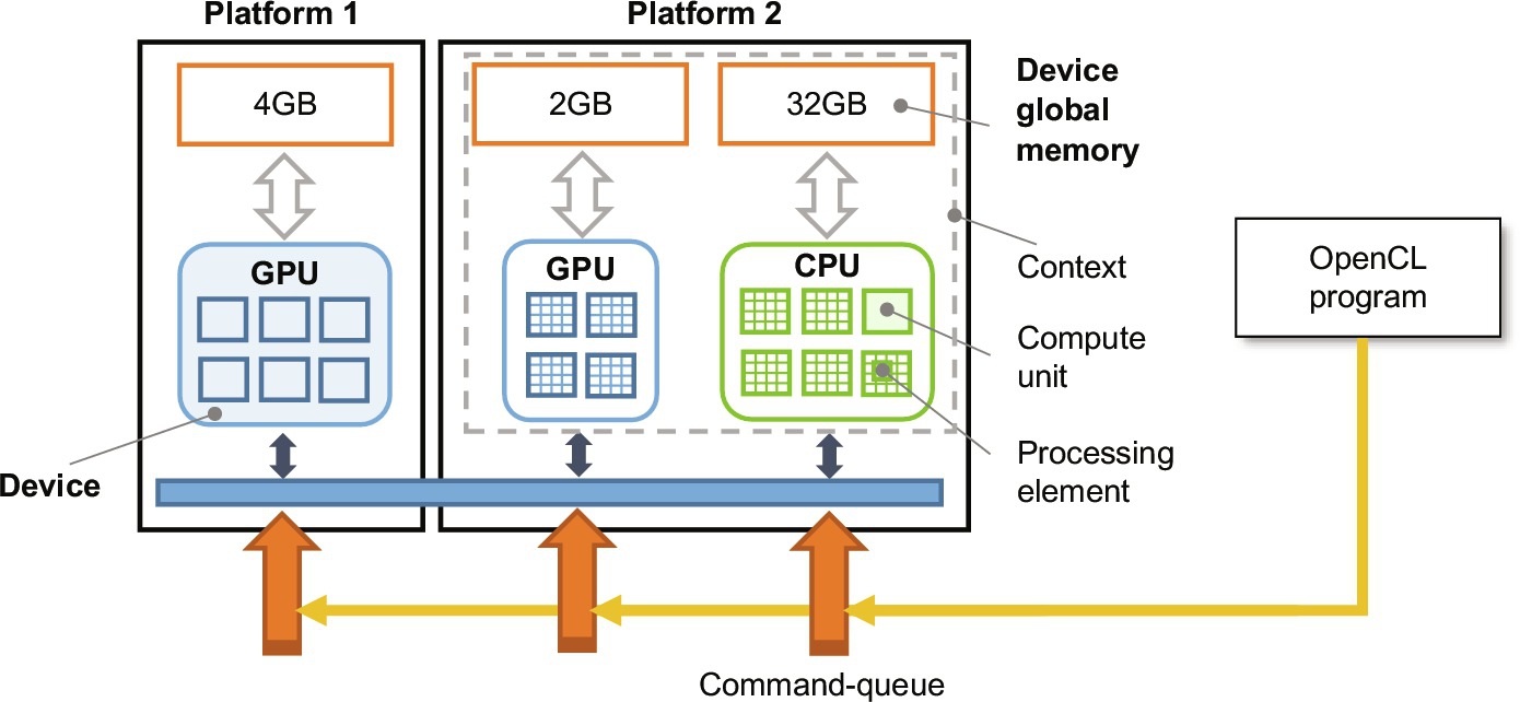
To deploy and execute an OpenCL program into one or more devices, OpenCL supports two important concepts. First, a context which groups a set of devices from the same platform, allowing them to share the same OpenCL objects, such as memory and programs, and thus support the management of multiple devices from a single execution context. Second, a command-queue which must be created on each device (within an execution context) to allow the host to submit work to the device. When using multiple OpenCL devices, developers are responsible for manually partitioning application workload and distributing each part across available devices according to their computational capacities. In addition, and while the OpenCL kernel specification can be deployed to any device without modification, it is often modified, e.g., to take into account that CPUs have lower memory bandwidth but larger cache systems and support far fewer threads when compared to GPUs.

When the host sends workload to a device, it creates a kernel execution instance as illustrated in Fig. 7.7, where the kernel (along with its global and local dimensions) is deployed to the device. The global dimensions define the total number of work-items (threads) the device must compute. These work-items are combined into work-groups according to the local dimensions specified by the developer. Each work-group is executed by a compute unit, and each work-item is processed by one or more processing elements. The architecture of an OpenCL processing element depends on the type of device and its vendor, but it typically supports SIMD instructions. While the global dimensions are defined by the problem size, the choice of local dimensions can considerably affect overall performance since the number of work-items deployed to each compute unit has to be large enough to hide memory latency. The work-group size must also leverage available parallelism taking into account the number of processing elements within each compute unit and the number of compute units available in the device. For this reason, developers often perform design space exploration, experimenting different local dimensions to find the most performant configuration for a particular OpenCL device.

The OpenCL memory model is illustrated in Fig. 7.8. The OpenCL runtime assumes the existence of a host where an application is originally deployed and executed, and a set of OpenCL devices that handle offloaded computations from the host. The host has a main memory where the application data resides. On the other hand, each OpenCL device has four types of memories: (1) global memory which is the primary conduit for data transfers from the host memory to the device and can be accessed by all work-items, (2) constant memory where content can be accessed by all work-items as read-only, (3) local memory which is only accessed by work-items within a work-group, and (4) private memory which is specific to a work-item and cannot be accessed by any other work-item.

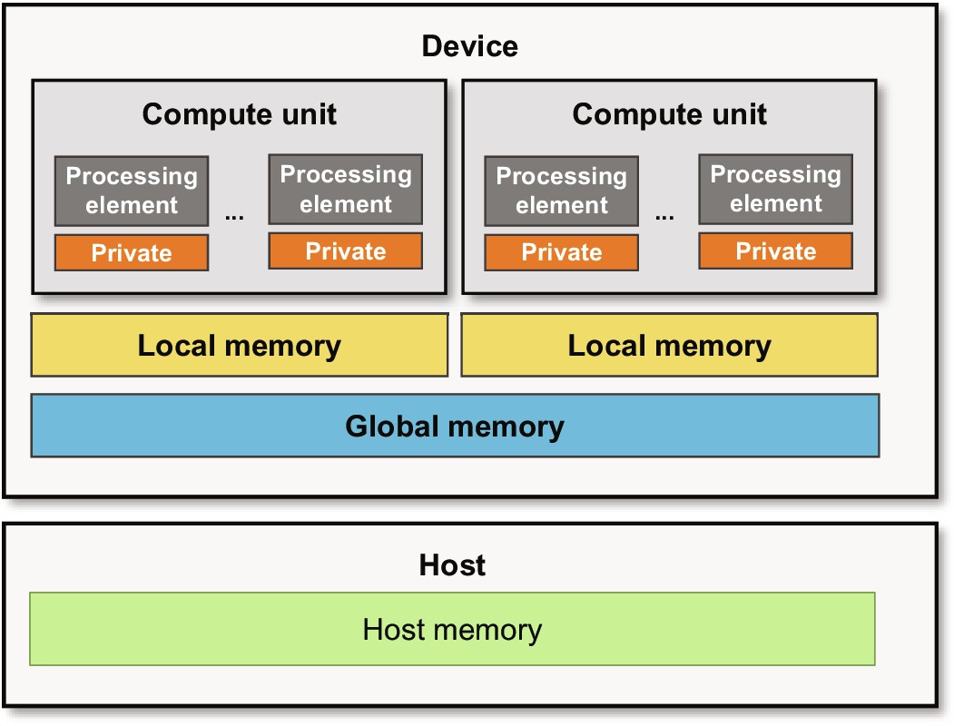
There is no automatic data movement in OpenCL. Developers are responsible for explicitly allocating global data, transferring data from the host memory to the global memory of the device, allocating local data and copying data from global to local memories and back, and finally transferring the results back to the host. When performing data movements, it is important to take into account both the size of memories and bandwidth. For instance, when the OpenCL device is connected to the host via the PCIe bus, transferring data from the host memory through the global memory can support bandwidths between 5 and 10 GB/s. Work-items can access the global memory with a bandwidth of 50–200 GB/s and the local memory at 1000 GB/s. Hence, caching data on faster memories can result in overall performance speedup. Modern GPUs support the option of automatically cache data to local memories, instead of manually managing it.

OpenCL implements a relaxed consistency memory model. This means work-items may have a different view of memory contents during the execution. Within a work-item, all reads and write operations are consistently ordered, but between work-items it is necessary to synchronize to ensure consistency. OpenCL offers two types of built-in functions to order memory operations and synchronize execution: (a) memory fences wait until all reads/writes to local/global memory made by the work-item prior to the memory fence are visible to all threads in the work-group; (b) barriers wait until all work-items in the work-group have reached the barrier, and issues a memory fence to the local/global memory. Note that synchronization support is limited to work-items within the same work-group. If synchronization between work-groups is required, should they share data in global memory, one solution is to execute the kernel multiple times so that memory is synchronized each time the kernel exits.

We now turn our attention to the matrix multiplication example presented in Section 6.1, that is, $\left(C=A\times B\right)$, and its mapping onto an OpenCL device. The most obvious OpenCL implementation strategy is to use two dimensions and allow each work-item to compute one element of the C matrix:

In this version, we use global memory to perform the computation over a 2D space. To further optimize performance, we use private and local memories which are considerably faster than global memory:

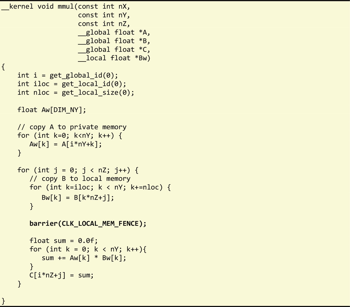
In this improved version, we operate in one dimension, so that each work-item computes one row of matrix C at a time. We note that for each row C, each work-item accesses a row of A exclusively. Hence, we copy the corresponding row from global memory to private memory (Aw) since it offers higher bandwidth than global memory. Note that the size of the private memory must be known at compile-time. In the above example, we specified DIM_NY as a #define constant (not shown), which must correspond to the value of nY supplied by the host.

Furthermore, since each work-item in a work-group also uses the same columns of B, we store them in local memory. Note that in the earlier code each work-item within a group copies part of the B column from global memory to local memory by referencing iloc (unique work-item index within work-group) and nloc (number of work-items within the current work-group). We then use a barrier to ensure all work-items within the group have a consistent view of B before each work-item computes a row of C.

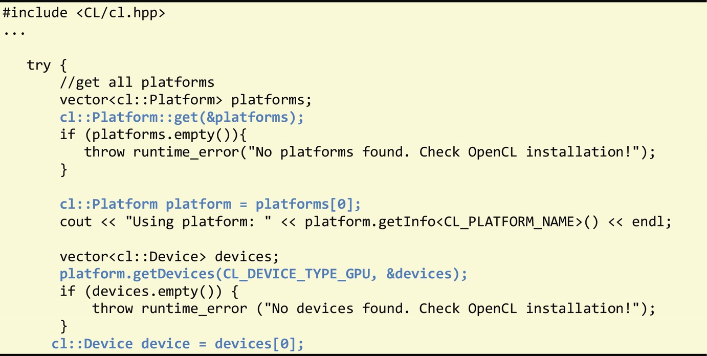
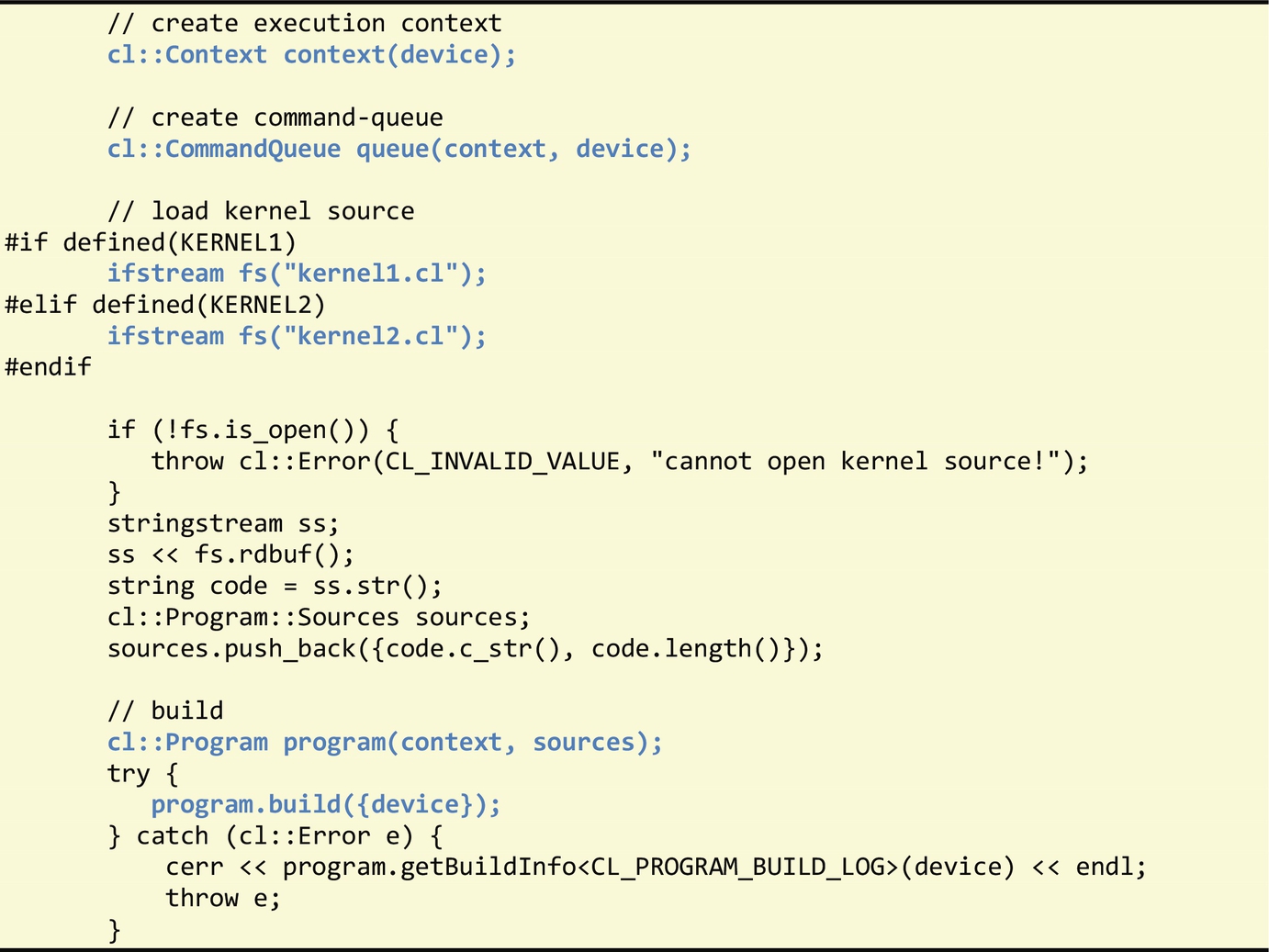
Regarding the host code, we use the OpenCL C++ wrapper API to deploy and execute the earlier kernels. In the following code, we select a GPU device from the first available OpenCL platform:

Once a device is selected, we create an execution context and a command-queue to deploy work to the device. Next, we load the OpenCL kernel source file and create an OpenCL program object and associate it to the execution context created earlier. Note that kernel 1 corresponds to the first version presented earlier, and kernel 2 corresponds to the improved version.

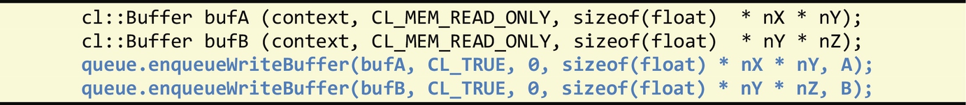
Next, we create buffers for matrices A and B with their respective sizes and submit a command through the command-queue of the device to copy matrices A and B from the host to the global memory of the device.

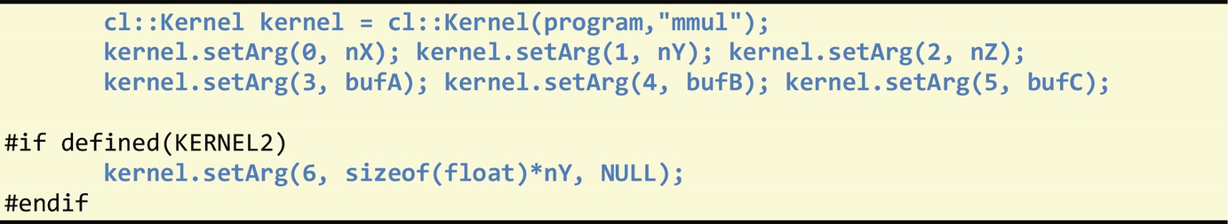
We then select the matrix multiplication (“mmul”) kernel and set the kernel arguments. Note that in the case of kernel 2, we pass an extra argument, which is the local array:

Finally, we execute the kernel by specifying the global and local dimensions and get the results back from global memory:

We finalize this section with a summary of techniques for exploiting OpenCL devices. First, one of the bottlenecks in performance is the data movement between the host and the devices working as coprocessors since the bus interfacing the devices might be slow. One common technique to minimize data transfers is to organize various kernels in a consumer-producer “chain,” in which intermediate results are kept in the device while running a sequence of kernels receiving as input the result of the previous executed kernel. Another important consideration is to use local memory instead of global memory since it allows almost 10 times faster accesses. For some devices, such as AMD GPUs and CPUs, the use of vector operations can have a huge impact in performance. Also, the use of half_ and native_ math intrinsics can help accelerate the computation at the expense of precision. Divergent execution can also reduce performance, which is caused when conditionals are introduced in kernels, and forces work-item branches (then and else parts) to be executed serially. Global memory coalescing also contributes to improve the performance as it combines multiple memory accesses into a single transaction, thus exploiting the fact that consecutive work-items access consecutive words from memory. Still, it is not always possible to coalesce memory accesses when they are not sequential, are sparse, or are misaligned. In this case, one common technique is to move accessed data to local memory.

7.5 High-level Synthesis

Compiling high-level program descriptions (e.g., C/C++) to reconfigurable devices (e.g., FPGAs), known as High-Level Synthesis or HLS, is a remarkable distinct process than when targeting common processor architectures, such as the x86 architecture. More specifically, software compilation can be seen as a translation process, in which high-level programming constructs are translated into a sequence of instructions natively supported by the processor. High-level synthesis, on the other hand, generates a customized architecture implementing the computations, described by the high-level program, using basic logic elements and their interconnections.

In general, the compilation of high-level programming languages to reconfigurable devices (see, e.g., [5–7]) distinguishes two types of targets: (a) fine-grained reconfigurable devices, and (b) coarse-grained reconfigurable devices or coarse-grained overlay architectures.

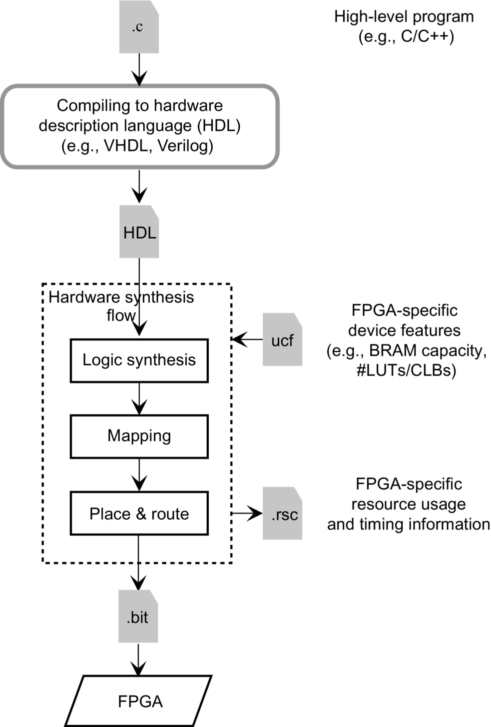
The HLS compilation flow [8–10] targeting fine-grained reconfigurable devices consists of a number of stages, as illustrated in Fig. 7.9. In the first stage, an RTL description is generated from a high-level program (e.g., a C/C++ program). An RTL model (usually described in a hardware description language such as Verilog or VHDL) represents a hardware design in terms of registers (Flip-Flops), memories, and arithmetic and logical components. In a subsequent stage, this RTL description is synthesized to logic gates (in a process known as logic synthesis [11]) and functional units directly supported by the FPGA resources. Next, these logic gates and the functional units are further mapped to FPGA elements (LUTs, Slices, BRAMs, DSP blocks, etc.). Finally, the placement and routing (P&R) process assigns these FPGA elements to actual resources on the FPGA and allocates the necessary interconnects between these resources to form a complete hardware circuit.

One of the benefits of mapping high-level computations to fine-grained reconfigurable devices, such as FPGAs, is the ability to select the best suited execution model and target custom architecture. As an example, the block diagram presented in Fig. 7.10 captures the structure of the edge detection implementation of the UTDSP benchmark introduced in Chapter 4. This block diagram exposes concurrency between tasks in the same stage (stages are identified in Fig. 7.10 with horizontal dotted lines) of this implementation. For instance, two convolve2d task instances can execute in parallel on two distinct implementations of the hardware elements that support their execution. When mapped to an FPGA, the computational nodes (elliptical-shaped nodes) are implemented as logic circuits with discrete elements, such as adders and multipliers, and their own Finite State Machine (FSM) controllers. On the other hand, storage nodes (rectangular-shaped node) can be implemented using on-chip FPGA memory resources (BRAMs), possibly using one memory per array, and in some cases using dual-port memories.

In addition to the task parallelism uncovered in this block diagram (Fig. 7.10), we can also leverage task-level pipelining. In a task-level pipelined execution mode, the computations are structured as a sequence of stages partially overlapped in time. Depending on the data accesses between producer and consumer tasks, the implementation can use FIFOs and/or memory channels to support communication between successive tasks.

There is in fact a substantial number of possible optimizations when using fine-grained reconfigurable devices, including the use of customized resources, code specialization, loop pipelining, and data parallelism. Furthermore, restructuring code (e.g., considering the code transformations presented in Chapter 5) and efficiently using HLS code directives allows the HLS tool to derive efficient hardware implementations when compared to their software counterparts.

Given the potential benefit of energy-efficient computing with reconfigurable devices, there has been a substantial investment in high-level synthesis (HLS) [13] in industry as well as an increased focus on academic research. At this time, and considering FPGAs as target devices and C/C++ code as the main input, there are academic tools such as the LegUp [14], as well as tools provided by FPGA vendors such as the Vivado HLS [12] by Xilinx [15], and tools provided by EDA companies (such as the Catapult C [16] by Mentor Graphics or the Impulse-C by Impulse Accelerated Technologies [17,18]). Recent trends include tools to map OpenCL computations to FPGAs and both Xilinx [19] and Altera [20] (now Intel [21]) provide such tools. Other commercial tools have focused on specific models of computation. This is the case with the MaxJ language and MaxJ compiler provided by Maxeler [22,23] which heavily relies on dataflow models of computation and streaming architectures targeting contemporary FPGAs.

One important aspect about fine-grained compilation to reconfigurable devices is the high computational and memory requirements for some of its compilation stages, in particular placement and routing. Developers used to fast software compilation cycles must contend with long compilation runtimes (several minutes to hours) required to synthesize a hardware design. Hence it is not always feasible to perform an exhaustive search of hardware designs. In this context, developers must understand the implications of source code transformations and compiler options before engaging the hardware compilation design flow.

The compilation flow targeting coarse-grained reconfigurable devices [24] or overlay architectures is fundamentally analogous to the flow described for fine-grained reconfigurable architectures, but often bypasses the hardware synthesis-related stages. In this context, Coarse-Grained Reconfigurable Arrays (CGRAs) [25] are the most used coarse-grained architectures, as they provide computing structures such as Processing Elements (PEs). These PEs provide their own custom instruction set architectures (ISA) which natively support word lengths of 16, 24, or 32-bit, and interconnect resources, between PEs and/or internal memory elements at the same word level. Because of their granularity, CGRAs impose additional constraints on how high-level computations are mapped to PEs, memory elements, as well as how their execution is orchestrated. Although the compilation of most CGRAs still requires a placement and routing (P&R) stage, this process is often less complex than when targeting fine-grained reconfigurable devices.

7.6 LARA Strategies

We now describe two strategies for improving the efficacy of the Xilinx Vivado high-level synthesis (HLS) tool. Both strategies first decide where to apply specific HLS optimizations, and then automatically apply these optimizations by instrumenting the code with HLS directives (see side textbox on Vivado HLS directives in the previous section).

The first LARA strategy (see Fig. 7.11) applies loop pipelining to selected nested loops in a program. As the Vivado HLS tool does not pipeline outer loops without fully unrolling all inner loops, when the PIPELINE directive is associated to a loop, all enclosed loops are fully unrolled. In the beginning of the strategy, all loop nests of a program are analyzed to decide where to include the PIPELINE directive. This is achieved by traversing all loop nests from the innermost to the outermost. For each traversed loop, the strategy invokes the aspect CostFullyUnrollAll (line 16) to decide about the possible feasibility and profitability of full loop unrolling. The CostFullyUnrollAll aspect (not shown here) estimates the complexity of the loop body (including all enclosed loops) if it were to be mapped to the FPGA. This complexity can be based on the number of iterations of the loops and on their body statements and operations. If the cost of the traversed loop is larger than the given threshold (supplied by the input parameter threshold), then the strategy instruments the code with the PIPELINE directive (see line 18) using the initiation internal (II) supplied by the input parameter II (with a default value of 1).

When this strategy is applied to a C code implementing the smooth image operator we obtain the code in Fig. 7.12, in which the PIPELINE directive is instrumented in the code using C pragmas.

The second LARA strategy (see Fig. 7.13) applies loop flattening (see Chapter 5) to perfectly or semiperfectly nested loops (starting from the outermost loop in the loop nest) while applying full loop unrolling to the remaining inner loops. This strategy mixes two strategies, one for selecting and applying loop flattening and another to apply full loop unrolling. For each traversed loop, the strategy acquires the information required to decide on the feasibility and profitability of full loop unrolling using the aspect used in the first LARA strategy (CostFullyUnrollAll). Also, this strategy can be easily extended to consider loop pipelining, thus making it applicable in a wider set of transformations contexts.

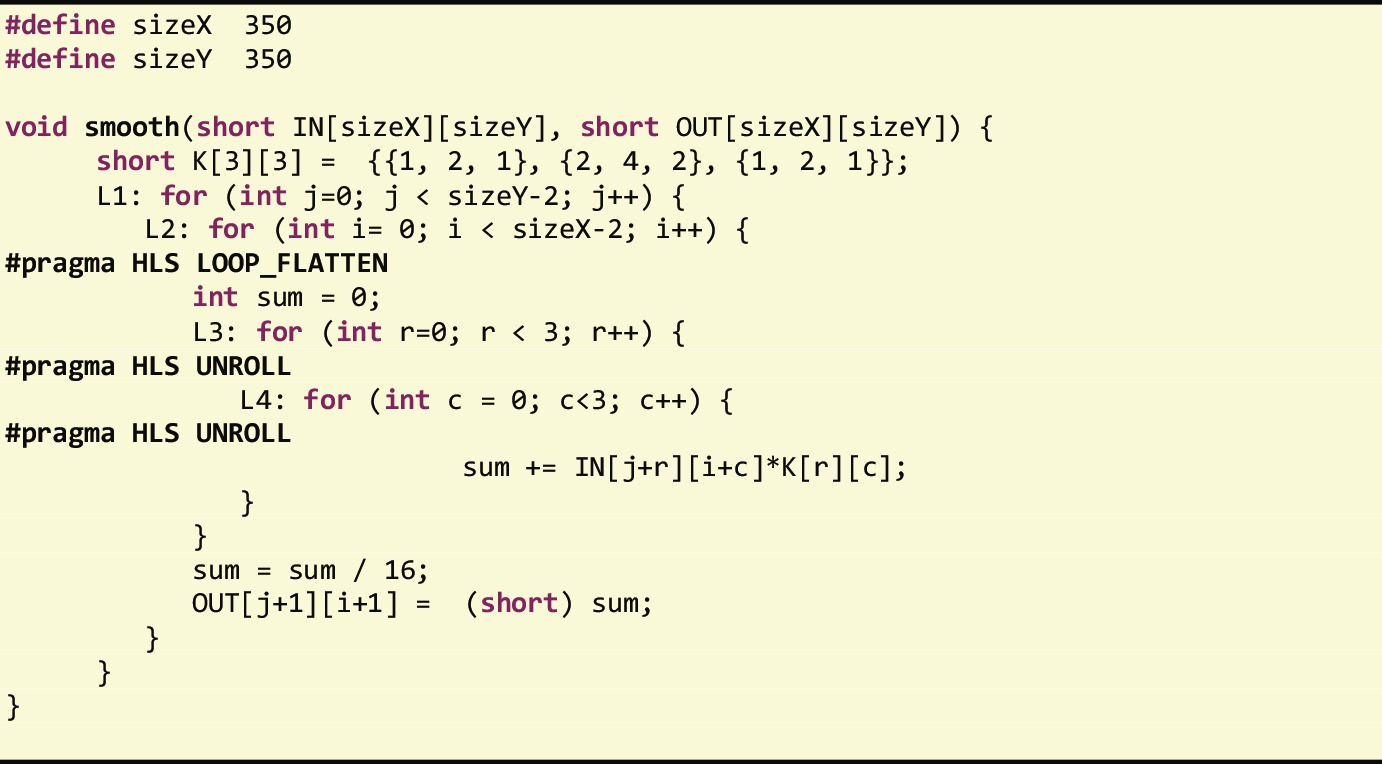
When this second strategy is applied to the smooth image operator example we obtain the code in Fig. 7.14, which includes the LOOP_FLATTEN and the UNROLL directives specified using C pragmas.

One of the key aspects of using LARA is that strategies can be extended or combined, thus increasing their transformational power and scope of applicability. This is clearly illustrated in the LARA strategy described earlier, which can be easily extended to consider loop pipelining in addition to the loop unrolling transformation.

7.7 Summary

This chapter expanded the topics on code retargeting for heterogeneous computing platforms, mainly leveraging the use of hardware accelerators such as GPUs and FPGAs. Special attention has been given to OpenCL and high-level synthesis (HLS) which translates C descriptions to hardware designs. The chapter revisited the roofline model and other performance models that aim at helping programmers with issues such as workload distribution and offloading computation to accelerators.

7.8 Further Reading

An excellent overview about reconfigurable computing is the book of Hauck and DeHon [5]. With respect to compilation to reconfigurable fabrics (such as FPGAs) the surveys presented in Refs. [6,7] provide a good starting point. A summary of the main high-level synthesis stages is presented in Ref. [8] but for a more in-depth description we suggest the book by Gajski et al. [13]. Readers interested in specific HLS tools can start by learning about LegUp [14], an available academic tool [9]. A recent survey comparing available HLS tools targeting FPGAs can be found in Ref. [26]. The impact of compiler optimizations on the generation of FPGA-based hardware is described in Ref. [27]. Details of the use of the Xilinx Vivado HLS tool are presented in Ref. [12] and the tutorials provided by Xilinx are important material source for beginner users of Vivado HLS.

For an introduction to the OpenCL programming model and its computing platform we suggest the material in Refs. [3,4]. Recent industrial development efforts on using OpenCL as the input programming model and underlying computing platform for FPGAs can be found in Refs. [19,20].