
Partitioning
There is always a point where a certain effect is the greatest, while on either side of this point it gradually diminishes. [Law of Diminishing Returns]
Thomas R. Malthus
The Corn Laws
The decomposition of a software reference design into two components — the portion to be realized in hardware and the portion that will run as software on the processor — is the essence of the partitioning problem.
For systems based on Platform FPGAs, partitioning is a subset of the more general problem addressed by hardware/software codesign. In codesign, hardware refers to the broader definition of hardware (physical, nonsequential, and possibly analog components) and, as such, involves assigning components of the application to a wide variety of devices with a wildly varying set of characteristics. Some may also be analog devices, which are unlikely to be specified in software. With the advent of Systemon-a-Chip (SoC) technology, many of these components are likely to be integrated on a single chip, but some may be discrete parts.
With the hardware/software codesign problem, the system designer must contend with issues such as interfacing continuous and discrete signals and electrical characteristics that are generally the purview of electrical engineers. Thus, hardware/software codesign is a very different (and much larger) problem than the partitioning of an application for a single, Platform FPGA. While some of the techniques described in this chapter may also be useful in hardware/software codesign, it is important that readers are aware that a complete treatment of codesign is beyond the scope of this chapter.
The learning objectives of this chapter are to:
• Understand the principles behind partitioning through the use of profiling and how to analyze performance while avoiding common profiling pitfalls.
• Build a formal mathematical formulation of the partitioning problem and provide a heuristic for maximizing the performance metric.
• Address issues associated with interfacing the hardware and software components of a decomposed software reference design.
• Focus on several pragmatic concerns not accounted for in the formal description of the problem.
Also note that this chapter only considers the static decomposition of a software reference design — dynamically decomposing a program is a research issue.
4.1 Overview of Partitioning Problem
To begin, let’s consider an application as a set of instructions organized as a collection of control flow graphs that specify the order of execution. The idea of partitioning is the grouping of specific sets of instructions in an application and then mapping those groups to either hardware or software. The groups assigned to software are executed sequentially (on a processor), while those mapped to hardware are implemented as custom combinational or sequential circuits and are realized in the configurable logic resources of the FPGA. If the application is a fully functioning software reference design, the result of partitioning is known as decomposition.
A number of factors help guide partitioning decisions. These include the expected performance gains (due to moving software into hardware), the resources used in the hardware implementation, how often that portion of the application is used, and — perhaps most importantly — how much communication overhead the decomposition introduces. Other pragmatic issues surface as well, including how difficult it is to implement a particular set of operations in hardware. In an ideal world, the groupings, mapping, and translation of instruction groups to hardware would happen automatically. However, state-of-the-art techniques are largely manual, with a handful of analytical and empirical tools to assist us.
We define a feature as a connected cluster of instructions from the application’s software reference design suitable for a hardware implementation. (We think of the hardware implementation as being an additional, application-specific architectural feature. Hence the name.) For the moment, we will leave suitable imprecisely defined to mean “the system designer anticipates that a hardware implementation will prove advantageous.” For now we can think of a feature as a subroutine from the software reference design. However, to achieve good partitionings, we generally have to examine groupings that may be bigger than or smaller than the subroutines defined by the programmer. In practice, a feature can vary from a few instructions to a “kernel” of nested loops to a whole software module consisting of multiple subroutines. Because feature size affects performance directly and indirectly, the decision of whether to implement a feature in hardware depends on its improvement to the overall system performance and the resources it uses relative to the other candidate features. If determined to be worthwhile, then the feature’s hardware implementation augments the hardware architecture.
To provide some context for what we are trying to do here, let’s consider a motivating example. The graph illustrated in Figure 4.1 depicts the execution of a JPEG2000 encoder application (Adams, 2007). From the main subroutine, we can see that 11% of the time is spent reading the source image and 89% of the time is doing the encoding. Encoding is not a single subroutine but rather a score of subroutines. If communication were free and hardware resources limitless, one would simply move everything into hardware. Given that neither is true, we have to determine which subroutines (or parts of subroutines) will have the biggest impact on some performance metric.

Figure 4.1 An encoding JPEG2000 image.
Profiling
The graph illustrated in Figure 4.1 was created by profiling the software reference design. To profile an application means to collect run-time information on an application during execution. With profiling, the software reference design is executed with representative input and the time spent in various parts of the application is measured. Profiling can be accomplished in a number of ways. Although it has been around for decades, it remains an area of active research as to optimize sequential program execution at run time. Here, we assume the simplest technique that profiles an application by periodically interrupting the program and sampling the program counter. A histogram is used to count how often a program is interrupted at a particular address in the application. From histogram data, an approximate fraction of total execution time spent in various parts of the application can be computed.
The Unix tool gprof is a good example of a sample-based technique. The default granularity for gprof is subroutines but it can also be configured to approximate the fraction of time spent in various basic blocks. Its output includes a flat profile of the percentage of time spent in each subroutine and a dynamic call graph that indicates which subroutines were invoked. (We’ll cover the practical details of using this tool in the gray pages of this chapter.)
Performance Analysis
Amdahl’s law, which is well known in computer architecture, applies the law of diminishing returns to the usefulness of a single architecture feature. In short, it is written

and it articulates the limits of the overall improvement to an application that a single enhancement can make on the execution time. By generalizing this to include all potential enhancements and an arbitrary performance metric, we can characterize the limits of a collection of enhancements. If these enhancements are hardware features and we can anticipate the required resources potential gain for each feature, then we can develop a model that will guide the partitioning process.
Amdahl’s law is not suitable because:
In Practice
Of course, the model is only as good as the data used to drive it. Sample-based profiling requires representative input and is an approximation of time spent. Without implementing all potential features in hardware, it can be difficult to anticipate the resources required. Often, we can analytically determine how many clock cycles a hardware feature will take and we can calculate a metric, such as speedup. However, in general, it is impossible to know when an arbitrary process will complete. Rather than provide an automated solution, the analytical solution simply provides a framework to guide a system designer to a creative solution.
4.2 Analytical Solution to Partitioning
This section mathematically formulates the problem of grouping instructions into features and then mapping those features to either hardware or software. The final task — converting the features into FPGA implementations — is included throughout this book. Presently, the most common way of performing this translation is to manually design the core with an HDL using the software reference design as a specification. Many vendors have recently announced tools that are intended to automatically synthesize HDL cores from high-level languages; however, as of this writing their suitability for our purpose and effectiveness have not been established.
Many practical issues impact the actual performance of a system. Not all of these issues can be incorporated into an analytical model — so, at best, we can only expect a mathematical solution will produce an approximate answer to the partitioning problem. Moreover, many of the inputs to our model are estimates or approximations themselves, which further degrades the fidelity of our results. So why bother? By first solving the partitioning problem “on paper,” so to speak, we get a partitioning that is close to optimal. From there, it is up to the designer to be artful in their use of guidelines and engineering expertise to refine the solution. In the end it is more efficient to use a combination of mathematical and ad hoc techniques to find an optimal solution than to simply rely on an engineer’s intuition.
As mentioned earlier, performance is a complex metric. However, to simplify the presentation in this section, we focus on just one facet of performance, improving the rate of execution (or speedup) over an all-software solution. Specifically, the goal of this section is to find a partitioning of the system to maximize the speedup. Our choice of speedup is motivated by the fact that it has the most fully developed set of empirical tools and, despite the comments of Chapter 1, it is the primary goal of many designs.
The approach taken here requires that some measurements be taken from the software reference design (application) and that certain characteristics of the potential hardware implementation(s) are known. Some of this information can be derived from analysis of the source prior to execution, but often a good deal must come from executing test runs and profiling the application. The principles for performance metrics other than speedup are similar.
4.2.1 Basic Definitions
In Chapter 3, we modeled a subroutine of a software reference design as a Control Flow Graph (CFG). This notation will be used again to represent the flow between basic blocks of a subroutine. In addition, this chapter extends that notation to include a Call Graph (CG), which consists of a set of CFGs (one per subroutine)
![]()
where ![]() is the CFG of subroutine
is the CFG of subroutine ![]() . The application’s (static) CG is then written
. The application’s (static) CG is then written
![]()
where ![]() . Two subroutines are related
. Two subroutines are related ![]() if it can be determined at compile time that subroutine
if it can be determined at compile time that subroutine ![]() has the potential to invoke subroutine
has the potential to invoke subroutine ![]() .
.
It is assumed that the basic blocks of every subroutine are disjoint: that is, every basic block in the application belongs to exactly one CFG. Moreover, it is assumed that a root node for the CG is implicit (i.e., one subroutine is distinguished at the start of execution). These are reasonable assumptions because, in practice, they are a natural artifact of how object files are created, stored, and executed.
On a practical note, not all executables can be expressed in this model. Certainly, system calls disrupt the control flow graph in unanticipated (and unrepresented) ways. Signal handling and interrupts are not represented. Some switch statements (i.e., case statements) are implemented as computed jumps. Thus, it may not be possible to determine all of the edges, ![]() , in a given subroutine’s Control Flow Graph,
, in a given subroutine’s Control Flow Graph, ![]() , before execution. Finally, the object-oriented paradigm relies on run-time linkages to invoke virtual methods. By design, this paradigm prevents us from knowing all of the edges before execution. For now, we assume that the model is complete enough to express a software reference design and we will return to these practical issues in the next section.
, before execution. Finally, the object-oriented paradigm relies on run-time linkages to invoke virtual methods. By design, this paradigm prevents us from knowing all of the edges before execution. For now, we assume that the model is complete enough to express a software reference design and we will return to these practical issues in the next section.
A second practical note: we chose basic blocks because, to date, empirical evidence suggests that there is not enough parallelism at the basic block level to warrant attention at a finer grain level. If this changes in the future, it is relatively simple to recast the problem in terms of instructions (or smaller) computation units. However, gathering performance data on units less than a basic block may present a practical problem.
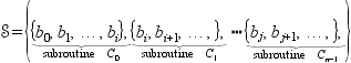
A common misconception is that a formal definition of partitioning only applies to the separation of an application into its hardware and software components. That is, the partition contains exactly two subsets. However, to make the problem more tractable, it is common to group operations into features first (a partition with a much larger number of subsets) and then map those features to either hardware or software. Assuming that the features are reasonably well clustered, then the decomposition of an application into hardware and software components can be driven by comparing the performance gains of features against one another.
First, let’s formally define a partition. (We use this definition again in Chapter 5.) A partition ![]() of some universal set
of some universal set ![]() is a set of subsets of
is a set of subsets of ![]() such that
such that
![]() 4.1
4.1
![]() 4.2
4.2
and
![]() 4.3
4.3
In prose, Equation 4.1 says that every element of ![]() is a member of at least one subset
is a member of at least one subset ![]() . Equations 4.2 and 4.3 say that the subsets
. Equations 4.2 and 4.3 say that the subsets ![]() are pair-wise disjoint and not empty. In other words, every element of our universe
are pair-wise disjoint and not empty. In other words, every element of our universe ![]() ends up in exactly one of the subsets of
ends up in exactly one of the subsets of ![]() and none of the subsets are empty.
and none of the subsets are empty.
For example, consider the set of English vowels, ![]() . One partition
. One partition ![]() of
of ![]() is
is
![]()
Figure 4.2 illustrates ![]() graphically. Another example is
graphically. Another example is
![]()
However,
![]()
are not partitions because ![]() violates Equation 4.1 and
violates Equation 4.1 and ![]() violates both Equation 4.2 and Equation 4.3.
violates both Equation 4.2 and Equation 4.3.

Figure 4.2 ![]() illustrated graphically.
illustrated graphically.
We can also apply this to an application ![]() . If we assume our universe is the set of all of the basic blocks from every subroutine,
. If we assume our universe is the set of all of the basic blocks from every subroutine,
![]()
then the subroutines partition ![]() . We will call this an application’s natural partition where
. We will call this an application’s natural partition where
Our task will be to reorganize the partition of basic blocks (and then map each subset to either hardware or software). We are free to create new (nonempty) subsets, remove subsets, and move basic blocks around until we have a new partition. The result is a new ![]() inferred from the reorganized partition
inferred from the reorganized partition ![]() . The second step is to map each subset of
. The second step is to map each subset of ![]() to either hardware or software:
to either hardware or software:
4.2.2 Expected Performance Gain
As we know, performance is not just a single number. However, to explain how performance can be used to guide partitioning, we choose a single metric — execution rate. This is partially motivated by the fact that the performance gain is relatively easy to measure and because, of all the metrics commonly used, speedup is often the most important one.
In the software world, performance is modeled all the time. The idea of complexity (order) analysis — that ![]() is better than
is better than ![]() — is widely understood and serves as an implicit guide when programmers everywhere compare algorithms. Unfortunately, the hardware world lacks that kind of general guide. Moreover, performance gain for the application may reside in the accumulation of many small gains that would be lost in a direct application of complexity theory.
— is widely understood and serves as an implicit guide when programmers everywhere compare algorithms. Unfortunately, the hardware world lacks that kind of general guide. Moreover, performance gain for the application may reside in the accumulation of many small gains that would be lost in a direct application of complexity theory.
Therefore, we use profiling information to collect the total execution time as well as the fraction of that time spent in each subroutine. The product is the approximate amount of time needed to execute that portion of the application in software and we use it as the time we expect it will take in future execution runs. We use ![]() to represent the expected execution time of one invocation of the subroutine (basic block)
to represent the expected execution time of one invocation of the subroutine (basic block) ![]() . It is an approximation for a number of reasons, not the least is that it depends on the input data set for many applications. However, there are also sampling errors that may impact performance. (Again, we refer to Section 4.4 for practical ways of improving the accuracy of
. It is an approximation for a number of reasons, not the least is that it depends on the input data set for many applications. However, there are also sampling errors that may impact performance. (Again, we refer to Section 4.4 for practical ways of improving the accuracy of ![]() .)
.)
Next we need to approximate the time that an equivalent implementation in hardware would take. In the case of a basic block, this is often much more precise. Without control flow (which, by construction, a basic block does not have), a synthesis tool can give a fairly accurate approximation of propagation time. Or, if the feature is pipelined, the number of stages is more precisely known. If the feature includes control flow but does not contain any loops, the longest path can be used as a conservative estimate. Features with a variable number of iterations through a loop present the biggest obstacle to finding an approximate hardware time. In this case, implementation and profiling with the hardware feature may be the only resort. Regardless, we assume that a suitable approximation ![]() for the hardware execution time exists.
for the hardware execution time exists.
Finally, the interface between software and hardware requires time and that cost needs to be accounted for as well. We can approximate this cost by approximating the total amount of state that needs to be transferred (if instantaneous transfer is used) or the setup and latency cost (if continuous transfer is used). In either case, it is represented by ![]() for feature
for feature ![]() . (More on the specifics of implementing and calculating communication cost between hardware and software is presented in Section 4.3).
. (More on the specifics of implementing and calculating communication cost between hardware and software is presented in Section 4.3).
Execution rate is the speed at which a computing system completes an application, and in a Platform FPGA system we look to hardware for improvement in the execution rate. This gain, which compares a hardware and software solution against a purely software solutions, is typically measured as speedup. We use ![]() to represent performance gain — whether the metric is speedup or otherwise — and this will allow us to compare different features against one another to determine the best partitioning. (Consequently, any subset of basic blocks that does not yield a performance gain can be generally excluded from consideration. In other words, only subsets of basic blocks for which
to represent performance gain — whether the metric is speedup or otherwise — and this will allow us to compare different features against one another to determine the best partitioning. (Consequently, any subset of basic blocks that does not yield a performance gain can be generally excluded from consideration. In other words, only subsets of basic blocks for which ![]() are considered candidate features.)
are considered candidate features.)
In general, we do not measure execution rate but rather the execution time, which is the inverse. So when considering whether a particular set of basic blocks should be mapped to hardware or software, we are interested in the gain in speedup, or
![]()
More specifically, we are interested in the performance gains of individual features, so we define ![]() ,
, ![]()
![]() 4.4
4.4
where ![]() and
and ![]() are the execution times of a hardware and software implementation of feature
are the execution times of a hardware and software implementation of feature ![]() . The function
. The function ![]() is the time it takes to synchronize affected, trapped state, that is, the time it takes to marshal data between processor and reconfigurable fabric.
is the time it takes to synchronize affected, trapped state, that is, the time it takes to marshal data between processor and reconfigurable fabric.
Let’s assume for the moment that we just use this single feature in our design. How much faster is the application? This depends on both the performance gain of the feature and how frequently it is used in software reference design. We can get this fraction of time spent in a particular feature, ![]() , from the profile information. The overall speedup of the application will be:
, from the profile information. The overall speedup of the application will be:
![]() 4.5
4.5
(Note the inversions again; we are moving between execution time and rates of execution to keep the sense of “performance gain.”)
From this equation, we can observe that increasing the hardware speed of a single feature has less and less impact on the performance of the application as its frequency decreases. To increase the overall system performance of the application, we also want to look at another dimension: augmenting the system with multiple features that will increase the performance of individual components as well as increase the aggregate fraction of time spent in hardware. Recognizing this, we want to compute the speedup of multiple features in hardware. In other words, we want to evaluate the system gain of a set of features ![]() where each member of the set contributes to the system performance based on the fraction of time spent in that feature. To estimate the performance of a partition, we can add features and rearrange the terms to get the overall expected performance gain,
where each member of the set contributes to the system performance based on the fraction of time spent in that feature. To estimate the performance of a partition, we can add features and rearrange the terms to get the overall expected performance gain,
 4.6
4.6
One might recognize Equation 4.6 as the the Law of Diminishing Returns first put forth by Thomas Malthus in the 16th century and Equation 4.5 is simply Amdahl’s law that we stated at the beginning of the chapter.
4.2.3 Resource Considerations
Following Equation 4.6 reductio ad absurdum, one would attempt to continue to add features so that ![]() approaches one. In other words, implement everything in hardware to maximize performance! Ignoring development costs (a very real constraint), there is a deeper issue of limited resources. On an FPGA, there are a finite number of resources available to implement hardware circuits. These resource are limited and most realistic applications will far exceed the resources available. Thus, given a large number of features, designers are often forced to limit the number of features implemented in hardware based on those that make the most impact.
approaches one. In other words, implement everything in hardware to maximize performance! Ignoring development costs (a very real constraint), there is a deeper issue of limited resources. On an FPGA, there are a finite number of resources available to implement hardware circuits. These resource are limited and most realistic applications will far exceed the resources available. Thus, given a large number of features, designers are often forced to limit the number of features implemented in hardware based on those that make the most impact.
One way of approximating resources is to count the number of logic cells required by each feature. So a chip will have a scalar value ![]() that represents the total number of logic cells available (after the required cores have been instantiated). Then
that represents the total number of logic cells available (after the required cores have been instantiated). Then ![]() can be used to represent how many logic cells each feature
can be used to represent how many logic cells each feature ![]() requires. A simple relationship,
requires. A simple relationship,
![]()
constrains how large ![]() can grow.
can grow.
However, we know that modern devices are heterogeneous. A typical Platform FPGA has multiple types of resources: logic cells of course, but also on-chip memory, DSP blocks, DCMs, MGTs, and so on. A vector,

is a better representation.
For example, the Virtex 5 (XC5VFX130T) has (this is not a comprehensive list, just a subset of all of the available types of resources):

We also promote the resource requirements function to a vector where ![]() represents the resources required by the feature
represents the resources required by the feature ![]() . Our new resource constraint equation is very similar:
. Our new resource constraint equation is very similar:
![]() 4.7
4.7
where ![]() is the set of features included in the design.
is the set of features included in the design.
Unfortunately, this model is somewhat idealistic as well. It does not take into account the fact that allocating some resources (such as BRAMs) may interfere with other resources (such as multipliers). Moreover, performance estimates are often based on the assumption that the resources allocated are in close proximity to one another. That is to say that routing resources are not an integral part of this model.
4.2.4 Analytical Approach
We now have the mathematical tools needed to describe the fundamental problem of partitioning. We first formally describe the problem in terms of the variables just defined and then describe an algorithm that finds an approximate solution.
Problem Statement
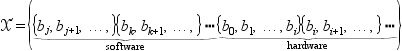
The basic idea is to find a partition of all of the basic blocks of the application and then separate those sets into hardware and software. Formally, we are looking for a partition ![]() of all the basic blocks
of all the basic blocks ![]() of the application:
of the application:
![]()
A subset, ![]() , where
, where ![]() is the vertices of the call graph
is the vertices of the call graph ![]() of the software reference design, is called the candidate set and contains all of the potential architectural features, that is, the subsets of
of the software reference design, is called the candidate set and contains all of the potential architectural features, that is, the subsets of ![]() that are expected to improve system performance if implemented in the reconfigurable fabric. Due to limited resources, we need to further refine this to a subset
that are expected to improve system performance if implemented in the reconfigurable fabric. Due to limited resources, we need to further refine this to a subset ![]() that maximizes our performance metric,
that maximizes our performance metric,
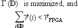
Algorithmically, one could approach this problem by finding all partitions of ![]() , synthesizing and profiling each partition, and then quantitatively evaluating every
, synthesizing and profiling each partition, and then quantitatively evaluating every ![]() . However, a simple application might have anywhere from 10,000 basic blocks to upward of
. However, a simple application might have anywhere from 10,000 basic blocks to upward of ![]() . This means that the number of partitions to evaluate is approximately
. This means that the number of partitions to evaluate is approximately ![]() ! Clearly, a brute-force approach is intractable. However, when one considers the fact that most of the inputs are estimates, the idea of relying on a heuristic is not disagreeable.
! Clearly, a brute-force approach is intractable. However, when one considers the fact that most of the inputs are estimates, the idea of relying on a heuristic is not disagreeable.
Heuristic
The partitioning problem is essentially a matter of indirectly manipulating the parameters ![]() and
and ![]() by rearranging the partitioning
by rearranging the partitioning ![]() . Then we select elements of
. Then we select elements of ![]() that meet our resource constraints and maximize our overall system performance
that meet our resource constraints and maximize our overall system performance ![]() .
.
A heuristic that can be applied informally is to start with the natural partition provided by the software reference design. That is, we use the subroutines of the original application.
We use our profiling tools to determine the fraction of time spent in each subroutine. Then, by listing the subroutines in decreasing fractions of time, we focus on those subroutines with a large ![]() . We rely on our experience in developing hardware cores to estimate the
. We rely on our experience in developing hardware cores to estimate the ![]() — the performance expected from a hardware implementation — and we have a system gain estimate for each subroutine.
— the performance expected from a hardware implementation — and we have a system gain estimate for each subroutine.
Next, we want to iteratively manipulate the partition ![]() by creating new basic block subsets, merging subsets, and moving basic blocks from subset to subset. The basic idea is to look for changes that will either increase the fraction
by creating new basic block subsets, merging subsets, and moving basic blocks from subset to subset. The basic idea is to look for changes that will either increase the fraction ![]() or increase
or increase ![]() of a potential feature.
of a potential feature.
Fraction of Execution Time
The way to increase the fraction of time spent in a subroutine is by making the feature larger. This can be accomplished by initially looking for relationships in the call graph or (after the partition has been manipulated) by looking for relationships in the control flow graph that bridge subsets.
For example, suppose an application spends 0.5% of its time ![]() in subroutine
in subroutine ![]() and 0.025% in subroutines
and 0.025% in subroutines ![]() and
and ![]() . The fraction of time spent in
. The fraction of time spent in ![]() can be doubled by merging
can be doubled by merging ![]() ,
, ![]() , and
, and ![]() . (In software terms, functions
. (In software terms, functions ![]() and
and ![]() are inlined.) Of course, merging does not come without a price. First, it (usually) increases the number of resources used. This has the potential of negatively impacting system performance by displacing other features or simply becoming too large to fit on the chip. Second, as explained later, increasing the size of the subset may decrease speedup — again negatively impacting the overall system performance.
are inlined.) Of course, merging does not come without a price. First, it (usually) increases the number of resources used. This has the potential of negatively impacting system performance by displacing other features or simply becoming too large to fit on the chip. Second, as explained later, increasing the size of the subset may decrease speedup — again negatively impacting the overall system performance.
Performance Gain
To increase the performance gain of a feature, ![]() , one needs to look at the control flow graph of the feature and evaluate whether a change will make it more sequential or more parallel. Oftentimes, algorithms that are inherently sequential (due to the flow or control dependences between the operations) perform better on a processor (because processors do not have the overhead of configuration transistors and because they have been carefully engineered for these circumstances). Simply adding basic blocks may have the undesirable effect of increasing the sequential behavior of the feature, lowering its
, one needs to look at the control flow graph of the feature and evaluate whether a change will make it more sequential or more parallel. Oftentimes, algorithms that are inherently sequential (due to the flow or control dependences between the operations) perform better on a processor (because processors do not have the overhead of configuration transistors and because they have been carefully engineered for these circumstances). Simply adding basic blocks may have the undesirable effect of increasing the sequential behavior of the feature, lowering its ![]() . Conversely, making a feature smaller has the potential of increasing its performance gain.
. Conversely, making a feature smaller has the potential of increasing its performance gain.
In terms of the application, this means taking a subroutine ![]() and breaking it into two subroutines
and breaking it into two subroutines ![]() and
and ![]() where subroutine
where subroutine ![]() invokes
invokes ![]() . If
. If ![]() extracts the parts of
extracts the parts of ![]() that can be improved in hardware and leaves the sequential parts in
that can be improved in hardware and leaves the sequential parts in ![]() , then the
, then the ![]() of
of ![]() will be higher than the
will be higher than the ![]() of the original
of the original ![]() . Most likely, it will require fewer hardware resources as well.
. Most likely, it will require fewer hardware resources as well.
To see how this works in practice, consider a subroutine that takes 93% of the execution time and provides a performance gain of ![]() . As is, this would provide the application with a performance gain of
. As is, this would provide the application with a performance gain of ![]() . However, if part of the original subroutine can be extracted (and its parallelism increased), then it is entirely possible that the performance gain could go up by a factor of 10,
. However, if part of the original subroutine can be extracted (and its parallelism increased), then it is entirely possible that the performance gain could go up by a factor of 10, ![]() , while its fraction of execution time decreases to 83%. This partitioning gives us an overall system speedup of
, while its fraction of execution time decreases to 83%. This partitioning gives us an overall system speedup of ![]() . Ahmdal’s law teaches us to always try to increase the fraction of time spent in the “enhanced” portion of the code. However, as this example shows that, when limited, fungible resources are part of the equation, it is not always better.
. Ahmdal’s law teaches us to always try to increase the fraction of time spent in the “enhanced” portion of the code. However, as this example shows that, when limited, fungible resources are part of the equation, it is not always better.
It is also important to note that any change to the subset may affect performance by increasing or decreasing the marshaling costs. That is, merging two subsets could dramatically increase the performance gain because less data have to be explicitly communicated between the processor and the feature. However, the exact opposite effect is possible as well. Moving basic blocks from one subset to another may result in a larger affected state.
Thus, in summary, the general heuristic works by examining the CG and CFGs of the application and then making incremental changes to the subset of the partition. Changes are guided by:
4.3 Communication
When a single application is partitioned into hardware and software components, it is necessary for those components to communicate. It is now important to discuss a number of issues related to communicating state across partition boundaries and the mechanism for transferring control between hardware and software.
Consider an application consisting of several subroutines. One particular subroutine might involve many simple bit manipulations such as the error-correcting code shown in Listing 4.1. It is reasonable to expect that a hardware implementation of this subroutine will substantially outperform the best software implementation and require relatively few FPGA resources. Hence, the subroutine hammingCheck is identified as a potential feature and its hardware implementation becomes a candidate for inclusion in the final system. However, we stress candidate because again, at this point, even though it may improve the system, we have a limited number of resources and it may not be part of the most beneficial decomposition.
Listing 4.1 A simple error-correcting subroutine
class HammingCheck {
public static byte hammingCheck(byte d, byte check) {
int my_check;
byte err_loc;
my_check=(((d![]() 7)^(d
7)^(d![]() 6)^(d
6)^(d![]() 4)^(d
4)^(d![]() 3)^(d
3)^(d![]() 1))&1) |
1))&1) |
((((d![]() 7)^(d
7)^(d![]() 5)^(d
5)^(d![]() 4)^(d
4)^(d![]() 2)^(d
2)^(d![]() 1))&1)
1))&1)![]() 1) |
1) |
((((d![]() 5)^(d
5)^(d![]() 5)^(d
5)^(d![]() 4)^(d
4)^(d![]() 0))&1)
0))&1)![]() 2) |
2) |
((((d![]() 3)^(d
3)^(d![]() 2)^(d
2)^(d![]() 1)^(d
1)^(d![]() 0))&1)
0))&1)![]() 3);
3);
err_loc=(byte)(check^(byte)my_check);
switch(err_loc) {
case 0:
//No error
break ;
case 1: case 2: case 4: case 8:
//Error in parity bit (data OK)
break ;
case 3:
return((byte)(d^0x80));
case 5:
return((byte)(d^0x40));
case 6:
return((byte)(d^0x20));
case 7:
return((byte)(d^0x20));
case 9:
return((byte)(d^0x8));
case 10:
return((byte)(d^0x4));
case 11:
return((byte)(d^0x2));
case 12:
return((byte)(d^0x1));
}
return(d);
}
}
Assuming that we have implemented this feature in hardware, the key question of this section is: how does this feature and processor interact? The set of rules that govern this interaction is called the interface; it is described in Chapter 2. Standard interfaces abound — such as how to pass arguments on the stack or the format of a network packet — and, most likely, readers have never considered defining their own low-level hardware interface. However, with Platform FPGAs, it is up to the designer to either choose a predetermined interface or design a new one for each feature. Often, this decision is crucial: the interface can make or break the performance advantages of using FPGAs.
Adding a feature to the system requires that the processor and the feature maintain a consistent view of the application’s data. Collectively, all of the application’s storage (variables, registers, and condition codes, as well as I/O device configuration and FPGA configuration) at any specific moment in time is called its state. This is similar to the concept of “the context of a process” in multitasking operating systems. However, when multitasking in the single processor world, the same hardware is time-multiplexed so that an application’s state is generally accessible all of the time. Similar to the case where a collection of independent processors need additional mechanisms to keep state consistent, so do independent components in our Platform FPGA-based system. This issue is more complicated for features implemented in Platform FPGAs because (i) the embedded processors are not designed for use in multiprocessor systems, (ii) features have limited ability to directly access state inside the processor, and (iii) the nature of hardware design distributes state throughout the whole feature (instead of keeping it in centralized, named registers). Thus, interfacing is what allows a feature and the processor to communicate changes in state and is necessary to keep an application’s data consistent. In developing the software reference design, a programmer is not likely to think about these issues. The specification uses a sequential model, which may or may not express any concurrency and a single memory hierarchy is assumed. However, if consistency is not explicitly maintained by the designer’s interface between a feature and a processor, then the resulting system risks producing incorrect results. To reiterate the importance of the interface: every component of the system may work properly by itself but if the interface fails, the system as a whole may fail.
As a concrete example, consider the example in Listing 4.1 again. The interface could be as simple as transferring two bytes to the hardware core, signaling the core to start, and then waiting for the result. This highlights the two main issues of the interface:
The former is the subject of subsection 4.3.1 and the latter is the subject of subsection 4.3.2.
4.3.1 Invocation/Coordination
In a sequential computing model, the most common form of invocation is the subroutine call. The linkage usually takes the form of saving the return address and then branching to the address of the subroutine. Because the traditional (single) processor only maintains one thread of control, the caller is viewed as temporarily yielding control, which is returned when the subroutine finishes. Alternatively, the multithreaded programming model augments this invocation mechanism. Individual threads of control can invoke subroutines but also have the ability to fork a new thread of control and different threads communicate through a variety of well-known mechanisms (semaphores, monitors, etc.)
These two software concepts can be extended to hardware in terms of a coordination policy. Hardware is different from software in that there is no thread of control: generally, hardware is controlled by some state machine that is always “on”. However, most state machines have some sort of “idle” state and transfer of control can be thought of as leaving and entering the idle state. So the idea of transferring control is conceptual — the real issue is coordination. In general, there are three common approaches to coordinating hardware and software components. The dominant approach is the coprocessor model; however, the multithreaded and network-on-chip models are gaining acceptance. Each is described next.
Coprocessor Model
The coprocessor model (also known as a go/done model or client/server model) is similar to traditional subroutine call linkage. In this model, the hardware sits in an idle state, waiting to provide a service to the processor. The processor signals for the feature to begin and then waits for a result from the feature. These signals are often called go and done (which give rise to one name for this model).
To implement the go/done model, every feature is designed to have an idle state. In the go/done model, every hardware component has an idle state where it is, in essence, off. That is, the designer treats the hardware like a sequential model and there is a time-ordered transfer of control. It has a go signal that can be implemented as a single I/O line or as part of a more complicated interface (such as a FIFO). The general protocol is for the processor to signal to the hardware to begin. The current (operating system) process blocks itself. When finished, the hardware component signals “done,” which unblocks the invoking process. The hardware goes back into the idle state, waiting for another go signal. A variation on this model has the hardware component interfaced to other hardware components or external I/O. In this case, the component may be concurrently gathering statistics or serving autonomous functions independent of the processor. (For example, the component may be counting external electrical pulses over a period of time to compute the frequency. The go/done interface is only used when the processor needs to know what current frequency is.)
An important consideration in the go/done model is how to handle the time while the feature is operating. There is a range of ways to handle it based on how long it is expected that the feature will take to complete and system overheads (such as a bus transaction or an operating system call).
Fixed Timing
For small features that take a fixed, short amount of time to complete, the most efficient mechanism is for the processor to simply do an appropriate number of “no-op” instructions and then retrieve the results (perhaps checking that done was actually signaled). Oftentimes, the hardware is so fast that by the time the state has been communicated, the hardware has results for the processor.
Spin-Lock
When the amount of time a feature runs is unknown, mechanisms such as a spin-lock can be used. The processor uses a loop to repeatedly check some condition, indicating hardware has completed its computation. This is also known as polling hardware for its results. However, checking the condition frequently (commonly implemented as a “done” signal) may have the unintended consequence of slowing the feature by taking bus cycles away, for example.
// Simple y = m*x + b Example
invoke_hw(m, x, b);
while(!done) {
done = check_done_signal();
}
y = retrieve_results();
Blocking
The traditional way of handling this situation is to treat the feature like an I/O device. The “done” signal can be routed as an interrupt to the processor. Then the feature can transfer the inputs to the feature and then tell the OS to deschedule it until the feature completes.
// Simple y = m*x + b Example
invoke_hw(m, x, b);
yield();
y = retrieve_results();
One limitation of the coprocessor model is that it provides an asymmetrical mechanism. Figure 4.3 shows the four combinations how software and hardware may transfer control. The shaded lower half of the figure shows transfer-of-control mechanisms that are not always supported.

Figure 4.3 Transfer of control between hardware and software.
Special Solution to Coprocessor Model
Transferring state from hardware to software is often impractical. One way of identifying candidate features is described here. By ordering the methods first, the algorithm focuses on the most likely locations for feature extraction.
A (static) call graph ![]() of the application is constructed. Recursion is detected by finding the strongly connected components of
of the application is constructed. Recursion is detected by finding the strongly connected components of ![]() and removed from consideration. For example, print and list in Figure 4.4 form a strongly connected component and are marked with an
and removed from consideration. For example, print and list in Figure 4.4 form a strongly connected component and are marked with an ![]() . Next, the remaining vertices of
. Next, the remaining vertices of ![]() are assigned an ordinal by the rule,
are assigned an ordinal by the rule,

In other words, every node is labeled with the maximum integer distance from a leaf. For example, sar is ![]() rather than
rather than ![]() in Figure 4.4.
in Figure 4.4.

Figure 4.4 Example call graph.
Multithreaded Model
Increasingly, the multithreaded model has emerged as an important programming model. In systems with multiple processors, an operating system can manage multiple threads of control (operating within the same process context) to improve performance. In other situations, such as graphical user interfaces, the model has proved to be a productive programming one.
In the threading model, the true parallel nature of the hardware is acknowledged and the designer recognizes that the processor and hardware components are both running continuously. Coordination of these components is handled by the communication primitives that have been developed for concurrent processes: semaphores, messages, and a shared resource such as RAM. In this case, every hardware component is considered to be running as a parallel thread. A set of system-wide semaphores are used to keep hardware and software threads consistent. Instead of sitting in an “off” state, hardware conceptually sits in a blocked state waiting on a semaphore or for a message.
Network-on-Chip Model
Again, borrowing from the multiprocessor world, researchers are beginning to investigate a completely distributed state and rely on a message-passing to explicitly transfer state (subsection 4.3.2). In this model, coordination is implicit with the transfer of state. However, because this assumes that software reference design has been constructed with explicit message-passing commands, we do not consider it in an embedded systems textbook. Nonetheless, we have seen that high-performance computing techniques continue to filter down to the embedded systems, so it may be important in the future.
4.3.2 Transfer of State
Historically, maintaining consistent state across discrete FPGA devices and processors has been especially challenging. This is because each FPGA device had its own independent memory hierarchy, state is widely distributed in the design, and there is a wide variety of interconnects between FPGAs and processors (from slow I/O peripheral buses to high-speed crossbar switches). This is true with Platform FPGAs as well. (Although due to integration, it is possible to share more of the memory hierarchy.) This means less state has to be transferred and there are a greater variety of mechanisms available.
To explain these mechanisms, we define two concepts: affected state and trapped state. These concepts help us decide which parts of the application state need to be explicitly communicated between processor and feature.
Affected State
One of the first questions to ask is “What data need to be kept consistent?” For example, software compilers generate a large number of temporary variables that are used to hold intermediate values, and these values are often kept in registers (although they can be “spilled” into main memory). However, after serving their purpose as intermediate values, these data no longer contribute meaningfully to the state — only the final computation matters. Hence, some state is independent by construction and there is no need to transfer it. Other portions of state are simply not relevant to every computation; that is, not every portion of the application refers to every data value used. If we exclude these parts of the application state, what remains is the affected state. More precisely, we can define affected state as application data, during a transfer of control, that has the potential of being either read or written by either the feature or the processor. In other words, the affected state is the state we need to keep consistent.
For example, consider the (contrived) subroutine translate (a) in Figure 4.5 and a corresponding hardware implementation (b). This feature affects four int values in the application’s state. This includes the values stored in x, m, and b, as well as the return value of the function. For most processors, the compiler would have generated a temporary variable (call it t1) to hold the product ![]() to be stored in the general-purpose register of the processor. In hardware, this value would be expressed on a bus of signals between the multiplier and the adder (with the possibility of a register inserted). These values (corresponding to t1 and y in the software) are part of the state but are not necessary to maintain consistent state. Consequently the interface does not have to accommodate them.
to be stored in the general-purpose register of the processor. In hardware, this value would be expressed on a bus of signals between the multiplier and the adder (with the possibility of a register inserted). These values (corresponding to t1 and y in the software) are part of the state but are not necessary to maintain consistent state. Consequently the interface does not have to accommodate them.

Figure 4.5 Translate.
The subroutine translate might leave the false impression that the arguments and return values are the only parts of state affected by the subroutine. In functional programming languages this is true — it is called referential transparency — and it allows functions to be evaluated in local context with no global state to worry about. However, the dominant programming paradigm for embedded systems is imperative. In the imperative paradigm, identifying state can be much more difficult. (Indeed, for a wide range of reasons — from high-performance computing to computer security — identifying affected state is a major challenge.) Consider the subroutine1 of Figure 4.6 and the corresponding visual representation of state. Ignoring the presence of a cache, this example shows that part of the state resides in main memory. Because C handles arrays by reference and permits pointers to be used to freely access all of a process’s state, there are numerous ways for a single subroutine to affect the global state.
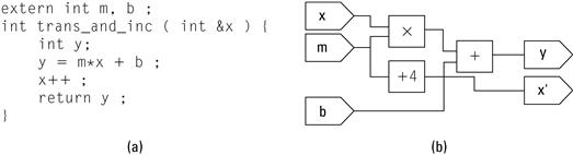
Figure 4.6 Translate and increment.
Trapped State
Unfortunately, the affected state can be quite large (especially if arrays, complex data structures, or pointers are involved). However, when part of the memory hierarchy is shared, not all data have to be explicitly transferred. For example, if all of the affected state currently resides in primary storage (RAM) and both processor and features have access to this part of the memory hierarchy, then there is no reason to explicitly transfer data.
However, modern processor designs are built with significant memory caches that can capture part of the state without updating primary storage. Compilers naturally take full advantage of the processor’s register set to hold state. Likewise, a hardware implementation typically embeds data throughout the design; registers and flip-flops hold intermediate values between clock cycles inside the design.
The state of an application is stored in several parts of a system. In the processor core alone, application data might reside in a general-purpose register, a cache, or (if an MMU is present and enabled) in a translation look-aside buffer. Outside the processor, application state might exist in on-chip Block RAM, in a subsystem buffer, or in external RAM. In order for a feature to implement part of the application, it will need to interact with part of the state. Sometimes this is accomplished easily because the state is in a common location (such as a common memory hierarchy). However, if that state is in a register or in the processor’s cache, it is usually not accessible to units outside the processor. We call this trapped state and it has to be explicitly transmitted across the interface. (The symmetric situation exists as well. Features are not required to be stateless — some of the application’s data may reside in a feature’s internal registers and that too would have to be communicated across the interface.) Figure 4.7 illustrates two places where state can be trapped.
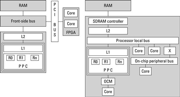
Figure 4.7 Two examples of where state can be trapped (a) traditional and (b) Platform FPGA.
This gives us a general idea of state, but before we begin to formalize the transfer-of-state problem, it is worth interjecting a brief discussion of pointers and the challenges faced in determining affected state. Often pointers are a source of frustration. They often confound automated translation techniques because the translator cannot tell if two pointers might refer to some location. Pointers also have the reputation of frustrating humans trying to analyze a piece of code (either to debug or to extend it). In both cases, it is a matter of intent — what did the original programmer wish to accomplish? In our situation, we can partially sidestep the intent problem without declaring pointers off limits because the sole purpose of a software reference design is to express intent. Pointers tend to obfuscate when used to improve performance in a clever way. But that effort is misspent in a reference design. So, while theoretically it is impossible to determine exactly what the affected state is, we will assume that in practice it is feasible because we have access to the original intent. Applying these manual techniques to “dusty deck” codes (older software that is still in use) may require more effort.
Transfer-of-State Problem
Affected state that is trapped needs to be explicitly communicated. This is done by a process called marshaling. Marshaling groups elements of the application’s affected state into logical records that are explicitly transferred. If we assume that the processor has control initially, there are up to four different kinds of records that may be used. The first two kinds are used to transfer an initial set of elements to the feature (Type-I, for initial) and a final set of elements back to the processor (Type-F, for final). These transfers take place when the feature is loaded and unloaded. Because all of the systems described are statically configured, these records are typically transferred at the very beginning of the application and when the application exits. The other two kinds of marshal records are used repeatedly — one when the feature is invoked (Type-CI, for copy-in), and the other when it completes (Type-CO, for copy-out).
For example, consider an MPEG encoder core. A matrix of quantization parameters is typically specified once for an entire application and those values do not change. Rather than transfer that state every time the encoder is invoked, those values can be transferred once at the beginning. For an example, consider the subroutine described previously in Figure 4.6(a). The Type-CI and Type-CO marshal records are shown in Figure 4.8. As an example of a Type-F record, suppose a core implemented in the configurable logic accumulates a value in a global variable (it may be statistics about its operation or samples it was given). A typical use of a Type-F record would be to read that variable after the last invocation.
![]()
Figure 4.8 Type-CI and Type-CO marshal records.
A translation process may be incorporated with marshaling. For example, floating-point numbers in the processor may be converted to fixed point when transferred to a feature. More complicated transformations, such as converting a linked list into a linear array of values are often appropriate. The grouping of elements is logical because the assembly does not strictly mean that elements are copied to a continuous location of memory. For small transfers, this is often simple and efficient. However, for many high-performance and multimedia applications, this is impractical. We describe a variety of techniques later.
The simplest way to transfer state is to copy the entire record, stop the processor until the feature completes, and then transfer the entire record back. This is considered a push, as the caller transmits data before transferring control. Alternatively, if a transfer record already exists and is in a known location in memory, then the caller can transfer control and the callee pulls data. One practical caveat: if the processor writes data to RAM and there is a cache, it has to also flush the cache.
For example, suppose the core is designed to find one element in an array. Depending on the algorithm, but under most circumstances, only a fraction of the array will be needed to complete the operation. Transferring the whole array when invoked is an expensive and unneeded operation.
Although simple, an instantaneous transfer of state is not always efficient or feasible. For example, oftentimes the size of the potential affected state is large but the actual data used are small. In this case, the data access pattern is random and the logical transfer record is large, but actual data are small. In this case, it is better for the interface to service the feature continuously. This occurs when both the logical record and the actual data record are large. If a large portion of data is expected to be used, then it makes sense to develop a regular access pattern that transmits data continuously. In such a scheme, the feature begins working on part of the transfer record while data are in transit.
In general, the choice of instantaneous versus continuous transfer is determined by the goal of the feature. Instantaneous is used when the feature is designed to reduce the latency of the task and the transfer record is small. Alternatively, continuous is used when the feature is designed to increase the throughput and latency reduction is not possible or not enough to meet performance targets.
Continuous transfer usually involves setting up DMA transfers and the incorporation of FIFO buffers. As such, it can increase the area and sometimes increase the latency. However, for many multimedia, signal processing, and scientific applications, throughput is the most important criterion.
One more fact is important with respect to transferring state. Often the best implementation in hardware uses a different format of data or possibly a different data structure. Translation is often an integral part of marshaling data.
Now that we understand the fundamental concepts of communication — coordination and state — we can take a formal approach to solving the partitioning problem. Armed with a detailed understanding of how to interface hardware and software components, we are now ready to tackle the partitioning problem directly.
4.4 Practical Issues
As mentioned at the beginning of Section 4.2, a mathematical model is suitable for getting us “in the ballpark.” However, there are numerous practical caveats and pitfalls that can confound the analytical approach. In general, experience and a few rule-of-thumb-type guidelines aid the system designer. This section highlights a number of these issues not addressed by the formal analytical solution.
4.4.1 Profiling Issues
A not-so-subtle assumption with analytical formulation is that it uses profile information to approximate the fraction of time that an application spends in a subroutine or basic block. However, a number of situations could generate misleading results.
Data-Dependent Execution
Some applications are stable in the sense that the fraction of time spent in each subroutine does not change substantially when the input is changed. However, for a number of applications — especially when the size of the input data set is changing or when the application responds to external events — a single data set will not be representative. In these cases, it is likely that the importance of various subroutines (based on their fraction of execution time) will change with respect to one another.
To detect this situation automatically is difficult. It requires the system designer to understand the fundamental operation of the application. For example, with applications that use many dense-matrix algorithms, the designer can analyze the complexity of various routines (i.e., “big-Oh” notation). For example, it may be the case, for small data sets, that two subroutines may take a similar fraction of time, but as the ![]() increases, a
increases, a ![]() subroutine will take an increasingly larger fraction of time relative to a
subroutine will take an increasingly larger fraction of time relative to a ![]() subroutine. Harder to analyze, but no less important, are applications that depend on external events. An example of this might be a handheld device: for some users, the phone will be the dominant mode, whereas for others Internet access might be the dominant mode.
subroutine. Harder to analyze, but no less important, are applications that depend on external events. An example of this might be a handheld device: for some users, the phone will be the dominant mode, whereas for others Internet access might be the dominant mode.
There are a number of ways to address these types of situations. One is to manually analyze the algorithms and understand the basic operation of the application. Another important tool is to collect profiling information based on a number of different (size and usage) data sets. A third is to try to separate the application, perhaps along module boundaries, and profile each module independently.
Correlated Behavior
Another subtle issue arises in some applications that explicitly use timed events. That is, many profilers implicitly assume that the application will make steady, asynchronous progress toward a solution. However, some applications are written to specifically incorporate time (such as event-loop and real-time systems). Because many profiling systems use an interval timer to sample the program counter, they rely on the application to be statistically uncorrelated to the timer. However, if the application is also executing operations in a regular, periodic fashion, then this is not true and profiling results may mislead the designer. For example, if events in the application are regular (occuring every 10 ms) and the samples are regular (the program counter sampled every 10 ms), then the profiler will not provide a statistically accurate description of the system. It could either over- or underrepresent a periodic event at the expense of other components in the software reference design.
Phased Behavior
It is well known that applications exhibit phased behavior: over the entirety of their execution, control moves between clusters of related operations. In other words, the execution of an application exhibits locality. Indeed, this characteristic, quantified by Denning & Kahn (1975), is commonly exploited in the design of computing systems. However, because of this, it may be difficult for the designer to identify important features from the summary numbers reported by a profiler.
As an example, consider an application that has three routines, ![]() ,
, ![]() , and
, and ![]() . Assume each account for 33% of the execution time, each has the possibility of being sped up by 50%, and the routines are ordered such that
. Assume each account for 33% of the execution time, each has the possibility of being sped up by 50%, and the routines are ordered such that ![]() runs to completion before
runs to completion before ![]() begins and
begins and ![]() completes before
completes before ![]() begins. If there is only room for one routine in the FPGA resources, then the maximum speedup for the system is 12%. However, if the phased behavior is recognized by the system design, then there are options. One is to look at commonalities among the three cores and try to find commonality. A second approach is to time-multiplex the hardware. No automated approaches exist to do this, but the last chapter of this book discusses how to perform run-time reconfiguration to “share” certain hardware resources.
begins. If there is only room for one routine in the FPGA resources, then the maximum speedup for the system is 12%. However, if the phased behavior is recognized by the system design, then there are options. One is to look at commonalities among the three cores and try to find commonality. A second approach is to time-multiplex the hardware. No automated approaches exist to do this, but the last chapter of this book discusses how to perform run-time reconfiguration to “share” certain hardware resources.
I/O Effects
Unforunately, most profilers do not account for I/O. This means that if the application spends a lot of time waiting for external events (such as network activity, reading/writing to disk, or waiting for user input), then improving the performance of computationally intense parts of the application may not yield the expected overall system performance gain.
For example, suppose an application consists of three subroutines — A, B, and C — and it takes 75 seconds to run. The profiler may report that 80% of the execution time is spent in subroutine C; however, that does not mean subroutine C takes 60 seconds! Why? Another useful utility time will help explain. Running the same application results in an output shown in Figure 4.9.

Figure 4.9 Time utility output.
Note that the “wall clock” (“real”) time is 75 seconds but the user time is only 22 seconds and the system time is 0.5 second. The user and system times represent how much time is actually spent inside of the application (in “user space”), and how much time is spent in the operating system (“kernel space”), respectively. Where’s the ![]() ? This is time that the application spent waiting on some external event. If the application is waiting for a user keystroke, that time is not counted against the user or system time — even though it does contribute to the overall wall clock time. Thus, a better estimate of the time spent in subroutine would be 80% of 22 seconds (17 seconds). Also any performance improvements gained from subroutine C will only improve 17 seconds of the total 75 seconds — not the original estimate of 60 seconds! So, while most profilers exclude I/O time and focus on just the computation time, the analytical formulation presented earlier implicitly assumes that we are trying to improve the computation rate of a compute-bound process.
? This is time that the application spent waiting on some external event. If the application is waiting for a user keystroke, that time is not counted against the user or system time — even though it does contribute to the overall wall clock time. Thus, a better estimate of the time spent in subroutine would be 80% of 22 seconds (17 seconds). Also any performance improvements gained from subroutine C will only improve 17 seconds of the total 75 seconds — not the original estimate of 60 seconds! So, while most profilers exclude I/O time and focus on just the computation time, the analytical formulation presented earlier implicitly assumes that we are trying to improve the computation rate of a compute-bound process.
Number of Calls
gprof and other profilers will also keep track of how often subroutines are called. It is important to note how often a subroutine is called because it can cause the profile information to vary wildly between runs. For example, it is common for applications to handle “special cases” differently. For example,
if( delta_t>MAX_SWING ) {
dim_display();
} else {
compute_accel();
update_display();
}
This code might be used to hide results when certain conditions suggest that data are not useful. Depending on data used to profile the software reference design, it may turn out that compute_accel() is only called once and has a small fraction of execution time. However, in practice, one would expect that the else-part of this code is the dominant path. The number of calls is a major clue to the engineer that perhaps the data set is not describing the behavior of the system accurately.
4.4.2 Data Structures
Software reference designs naturally reflect a bias toward software implementations. This is understandable, as programming is (appropriately) taught within the context of an ordinary sequential computing model. With such a model, the difference between
while( i!=NULL ) {
proc(i);
i = i->next;
}
and
while( i<n ) {
proc(x[i]);
i = i + 1;
}
is negligible: both take ![]() steps. However, with hardware, the latter is much more desirable. At minimum, a large prefetch window is possible. However, as we will learn in the next chapter, if we can determine that, in the various iterations of the loop, each proc(x[i]) is independent, then we could potentially improve the design through pipelining or regular parallelism so that the execution time approaches
steps. However, with hardware, the latter is much more desirable. At minimum, a large prefetch window is possible. However, as we will learn in the next chapter, if we can determine that, in the various iterations of the loop, each proc(x[i]) is independent, then we could potentially improve the design through pipelining or regular parallelism so that the execution time approaches ![]() steps.
steps.
What this example shows is another flaw in the analytical model of the previous section. The software reference design serves extremely well as a specification. However, if we simply profile the execution of the reference design, we do not capture the implementation benefits. Because these benefits come from algorithmic changes, it seems unlikely that automated techniques will reveal these advantages. Consequently, it falls on the system designer to understand both the software algorithm implemented in the reference design and how it might be reimplemented in hardware.
There are several places where common software structures can be rearranged to yield better hardware designs. For example, look for data structures that use pointers (linked lists, trees, etc.) and determine if they can be implemented “flat” structures (such as vectors and arrays). Flat structures produce regular memory accesses that can subsequently be prefetched or pipelined. Another place to look for performance gains is in bit widths. Software programmers generally assume a fixed, standard bit width even though they only use a few bits of information. This is because processors are slow at extracting arbitrary bits from a standard word. However, hardware excels at managing arbitrary bit widths. Finally, software has fixed data paths and (relatively) low bandwidth between components. When possible, consider leveraging the large bandwidth provided by the FPGA’s programmable interconnect.
4.4.3 Manipulate Feature Size
The simplest change involves breaking up subroutines into smaller subroutines. This has the effect of isolating computationally intensive parts of the subroutine (making the hardware feature smaller and easier to implement).
Alternatively, there are times when aggregating subroutines is needed. For example, if two subroutines each account for 25% of the application’s time, then they are strong candidates for hardware. However, if implemented individually, each invocation incurs the cost of interfacing. If these three subroutines are related (for example, one is also invoked after the other), then combining them into a single subroutine saves the cost of invocation. This happens frequently because ordinarily software programmers will break up subroutines to make the code more maintainable and the run-time cost of a subroutine is completely negligible. However, the cost of interfacing is not always negligible and it is worth the designer’s effort to investigate the situation.
Other changes are more substantial. Often the hardware implementation has a significant performance gain because it is better and has application-specific data formats. To make software more efficient in these nonstandard data formats, programmers will frequently employ data structures that do not map well to hardware. Thus, it is worth looking at the intent and considering replacing data structures to better exploit the hardware.
Chapter in Review
The aim of this chapter was to give readers a better understanding of the principles behind partitioning a software design into a more efficient and, if possible, faster hardware implementation. One technique introduced was profiling. We will actually see this tool more in Section 4.A; however, it provides a good indicator to what part(s) of the application may map well to a hardware implementation. Analytically, we built a mathematical formula of the partitioning problem and built a heuristic to maximize the performance.
Practical Expansion
Partitioning
In these gray pages, there are two main learning objectives. First, we describe a few of the practical issues of using profiling and the tool gprof. Then we build on the basic Linux system described in the previous chapter to add kernel modules.
4.A Profiling with Gprof
As mentioned in the white pages, one can get a statistical approximation of how much time a program spends in a subroutine relative to the overall execution time. In this section, we will look at how to use one specific profiler, demonstrate its use for a few applications, and then describe some more advanced tools for analyzing the behavior of a software reference design. Specifically, we will look at an application profiler and a system-wide profiler.
One of the easiest tools to use is the profiler that comes with GCC, called gprof (Graham et al., 1982). Gprof gathers three pieces of information during program execution: the number of times a subroutine is called, the execution time spent in each subroutine, and the dynamic call graph. (The static call graph described earlier in the white pages includes an edge between two vertices if there is the potential for one subroutine to call another. The dynamic call graph is a subset of vertices — excluding edges if a particular subroutine call was not invoked during execution.)
The first step in anlyzing a software reference design is to run it without gprof using the time command. (Time is a stand-alone application but is also built into some command line shells.) For example,
time sort -r /usr/share/dict/words > /dev/null
returns
real 0m0.657s
user 0m0.624s
sys 0m0.012s
What this means is that it took the sort command 0.657 second (wall clock time) to reverse the list of words in a dictionary file. Of the wall clock time, 95% of the time (0.624 second) was spent in the user’s program and 5% was spent outside the user space (either blocked on I/O or executing kernel code). In contrast, if we run
time cat /usr/share/dict/words > /dev/null
the output is
real 0m0.009s
user 0m0.000s
sys 0m0.008s
In this case, most of the time was spent outside of the user application. What is the difference here? In the case of sort, the application has a fair amount of work to do — sorting a bunch of strings, which is substantial compared to the I/O (moving data from the disk to the application). Computationally, the cat command is extremely simple — most of its time is literally spent alternating between the read system call and the write system call.
There are two immediate implications of this information. If the software reference design spends a substantial port of time in the operating systems (waiting on I/O, doing an intense number of system calls), then profiling the application as it is may be worthless. That is, looking for hardware accelerators in an application that is I/O-bound (instead of compute-bound) won’t yield any speedup. Second, the issue may be that, in the rapid prototyping stage, I/O was used to substitute for an instrument in the embedded system. For example, radar data may be the primary input to the system but the radar is not connected to the development machine running the software reference design. To simulate the radar, real data can be collected and stored in a data file. In this case, the software reference design is artificially I/O-bound and it may be possible to tweak the program to better represent its behavior in the embedded system. (A third possibility is that the application will be I/O-bound in the final embedded system. If this is the case, then this analysis tells the designer to shift emphasis from the computation to how the data is delivered. See Chapter 6 for more about managing bandwidth.)
Assuming the basic timing analysis suggests that the application is compute-bound, the next step is to profile the application. This is straightforward with GNU Compiler Collection — it will work even on the cross-development tools. (Of course, to get useful results can be a little more challenging; see next section.) There are three basic steps:
1. Add -pg to the CFLAGS environment variable. With a typical GNU package, this can be accomplished when the package is configured
./configure CFLAGS=-pg
Two potential snags to watch out for: (1) watch for the final link command — if the Makefile calls the ld command directly, you must include the -pg option to that command as well! Add LDFLAGS=-pg to the configure command will do this. (2) If there was a default CFLAGS in the configure (-g or -O2 are common) this overrides the existing options rather than augments them.
2. Run your application with inputs that are representative of what the embedded system will experience. The only catch here is that you have to have write priviledges in the current working directory at the end of the application. As long as the application exits normally, the there will be a gmon.out file with your profiling data. Note that gmon.out is overwritten every time you run the application.
3. The program gprof command interprets this data and produces two reports on the standard output. The command looks like this:
gprof −b myprog > myprog.stats
The -b option suppresses a long summary of the different comments. You may want this initially but after using gprof for a while, this option gives you just the data. (This command, as written, assumes that myprog and gmon.out files are in the current working directory.)
The output consists of two tables. The first table is a “flat profile.” The second shows the dynamic call graph. To understand what a developer can learn from these tables, let’s look at a several examples.
The first example comes from an implementation of an encryption/decryption standard called AES. This was compiled with the -pg option. Then the application was used to encrypt a 217MB CompactDisk image. The output from the profiler was gmon.out, and the gprof command, shown below, was used to convert the data file into a human-readable file.
gprof -b aespipe > data.stats
The first table from data.stats is shown in Figure 4.10. This is either very good news or disappointing news! It is clear from the flat profile that 8.12 seconds of the 8.65 seconds that the program ran was spent inside of one routine, aes_encrypt! If the AES routine was part of a bigger project, then this clearly identifies the routine to implement in hardware. However, if you were trying to partition AES on its own, then the single routine is all you have and none of the mathematical analysis of the white pages will help you.

Figure 4.10 AES flat profile.
Let’s look at another example. The Finite-Difference Time-Domain (FDTD) application simulates the propagation of an electromagnetic wave through some medium. For example, it might be used to simulate signals on the traces of a printed circuit board. After running it with profiling turned on we get the flat profile shown in Figure 4.11. One thing to notice is that six routines get called 20 times. This suggests that these routines are part of the main loop that iterates 20 times — in this case, it was the number of time steps simulated. It also tells you that these routines are the major procedures in the application. In this case, we probably also want to look at the dynamic call graph. Besides simply knowing where the time is spent, we would also like to know the invocation patterns to make sure we don’t spend all of our time marshaling data back and forth. We use a tool called Gprof2dot and the GraphViz package to convert the second table into a dynamic call graph. The resulting graph is shown in Figure 4.12.
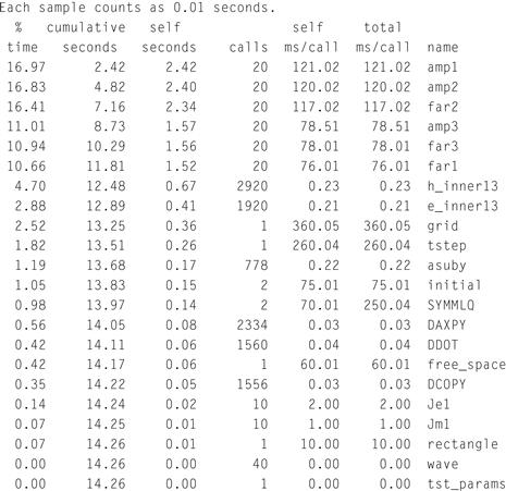
Figure 4.11 Finite-Difference Time-Domain simulation.

Figure 4.12 Finite-Difference Time-Domain dynamic call graph.
The last example, shown in Figure 4.13, presents an interesting case. It converts a PNM format image into a PGX format image. (PGX is a nonstandard format used by the JPEG2000 Verification Model software.) It is interesting to note that 53% of the time is spent decoding the PNM image. If we were to speed up the JPEG2000 encoding side, the best possible speedup would be ![]() and that’s assuming no communication cost and nearly instantaneous execution time in hardware!
and that’s assuming no communication cost and nearly instantaneous execution time in hardware!

Figure 4.13 JPEG2000 example.
We wrap up this discussion with a few final hints about profiling and related software tools. There is an art to profiling that involves figuring out what to profile. For example, sometimes it makes sense to profile a large subsystem in isolation. Most embedded systems would us JPEG2000 as a library, but in order to profile it, we needed a simple application that reads, converts, and writes a single image. Had the entire system been profiled together, a single subroutine may not have been so easy to spot. This was appropriate because we envisioned it being used with a camera that was continously producing data. In another application, it might not be appropriate.
Another issue that one might see with gprof is the presence of a mysterious function called mcount. This is the function that gets linked in when the application is compiled with -pg and it is used to keep track of how many times a subroutine is called. It is very short, so if it takes a large fraction of the run time, that suggests that the application is doing lots of subroutine calls and that the subroutines are short.
Using compiler optimizations requires some special attention as well. On one hand, if the application requires a certain level of optimization (-O3, for example) then one should profile it with optimizations turned on. However, the -O3 will automatically inline small subroutines — a change that will obviously distort the results.
Although we have focused on gprof, an Open Source profiler, there are others. Both AMD and Intel offer profilers that are especially well suited to their processors. AMD’s product is called CodeAnalyst and can be found at this Web site: http://developer.amd.com/cpu/CodeAnalyst. Intel’s product is called VTune and can be found at http://software/intelcom/en-us/intel-vtune. Two other Open Source profilers are called oprofile and Tprof. Part of the oprofile package is integrated with the Linux kernel and offers the ability to dynamically start and stop profiling. Another nice feature of oprofile is that the application does not have to be recompiled. Tprof is part of the Performance Inspector collection of tools (http://perfinsp.sourceforge.net/) and has the ability to run in two modes. Its time-based sampling is similar to gprof (periodically the process is interrupted). The second mode is event-based sampling. In this mode, the sampling interval is determined by how often a specific event occurs. Events that are counted could be cache misses, branches taken, or instructions retired. Increasingly, commercial processors are including counter registers throughout the processor and it seems likely that more event-based profiling will become an important tool to understanding the behavior of applications.
Finally, it is worth mentioning two very useful tools. A Python script called Gprof2dot (http://code.google.com/p/jrfonseca/wiki/Gprof2Dot) converts the output of gprof into a graph language called Dot. GraphViz (www.graphviz.org) reads a graph expressed in Dots and renders it visually in various graphics formats. These tools were used to create the figures in this section.
4.B Linux Kernel
4.B.1 Kernel Modules
There are two ways of extending the functionality of the the Linux kernel. The first is known as the “in-tree” approach. In this case, you get a copy of the kernel, pick a directory in the source code, and begin adding code to existing files or creating new files. The second approach is called “out-of-tree” and as the name suggests, you create new files in a new directory outside of the Linux source directory. The major difference is that with out-of-tree development, one must learn the interface and develop the extension as a kernel module.
It is slightly counterintuitive but the latter approach is usually preferable for first-time Linux developers. Regardless of which approach is used, one still has to learn the kernel build system and usually it will be necessary to learn the kernel module interface anyway. So the disadvantages are few but the big advantage is that an out-of-tree kernel module can be compiled and recompiled on its own. This makes testing easier. When the internal state of the Linux kernel is not corrupted by a bug, then it is possible to remove the kernel module, fix the source and recompile it, and then insert it again into the running system. Not having to reboot the system every time to fix small mistakes is much faster.
To use the kernel build system in the out-of-tree approach, one has to create a simple Makefile. The generic Makefile illustrated in Listing 4.2 is similar to the Makefile described in Corbet et al. (2005): the variable LINUX points to where the Linux source tree is and DRIVER_NAME is the name of the source file. In addition, we include the ARCH and CROSS_COMPILE to cross-compile the kernel.
The minimum components of a kernel module are shown in Listing 4.3. After including the header files, there are four preprocessor macros used to put identifying information into the kernel module’s object file. Next comes two subroutine — one is invoked when the kernel module is inserted, the other when the kernel module is removed. The kernel module does not use a reserved function name (like main in C) to identify the init and exit functions of a kernel module. Instead, the developer chooses them and tells the kernel with the last two preprocessor macros.
At this point, if one wanted to test their kernel module, one would create a base hardware system and compile a Linux kernel for this hardware. Then one uses the Makefile here to compile the hello.c into a “kernel object” called kernel.ko. This file is copied to the root filesystem before a filesystem image is created. Then you follow the steps described in the last chapter to create an ACE file or download the bitstream and kernel.
Once the system is booted, the developer can log in on the console and use the commands insmod ./hello.ko to insert a kernel module. The command rmmod hello removes it. (Note: In the former, the argument is a file name; the argument to rmmod is the name of a module.)
4.B.2 Address Spaces
One of the advantages of using a full-featured operating system is that each process gets its own address space. One of the disadvantages is that every process gets its own address space. In exchange for isolating software faults, it means we have to manage multiple address spaces in our kernel modules. This includes (at minimum) the physical address space (with respect to the system bus), the kernel’s address space, and the current running process’s (virtual) address space. The minimum one needs to know about moving data from one space to another in a device driver are these six routines:
1. request_mem_region(PHY_ADDR,LEN,“mycore”) / release_mem_region(PHY_ADDR,LEN, “mycore”)
2. ioremap_nocache(PHY_ADDR,LEN) / iounmap_nocache(PHY_ADDR,LEN)
The first pair of routines (1) mainly serve to catch misconfiguration errors. They simply alert the kernel that there is a range of physical addresses that this kernel module “knows” about and is claiming exclusive access to. (The third parameter gives a short text description of what is at that memory location.) If the two versions of a kernel module are accidentally installed twice, the second one will get an error when it requests the same memory range — this mechanism gives us a chance to catch that common mistake.
Requesting a range of physical addresses does not mean that the kernel has access to them. Even the kernel’s memory references are translated by the MMU into physical addresses. Consequently, we have to set up the MMU to translate our physical addresses into the kernel’s address space. Fortunately, the kernel provides ioremap_nocache to do this for us. (Whenever we are using physical addresses to communicate with an FPGA core, we want to be absolutely sure that the cache is turned off in that address range.)
The last two operations also protect a kernel module developer from a large degree of complexity. When the kernel is interacting with an application, the application will pass data through the system call interface. If that data is an addresss, then the kernel module will see it as a virtual address in the user process’s address space. Any local variables in the kernel module will be in the kernel’s address space. These two routines make it easy and efficient to move data between these two, distinct address spaces.
If the hardware device that you are trying to access was interfaced to the bus using the Add/Import Peripheral wizard, then the control registers are all going to be adjacent and start from some base physical address. Often the easiest way to keep track of the locations is to use a structure, such as the one below, and a pointer.
typedef struct {
volatile unsigned int reg0;
volatile unsigned int reg1;
volatile unsigned int reg2;
volatile unsigned int reg3;
volatile unsigned int reg4;
volatile unsigned int reg5;
volatile unsigned int reg6;
} mask_regs_t;
mask_regs_t *regs;
Then, assuming base and len are set to the base physical address and length of the memory region, the regs pointer can be set with
regs = (mask_regs_t *)ioremap_nocache(base,len);
To write a 0x00000001 to the third registers, one would write
regs->reg2 = 0x000000001;
Dynamic memory allocation in the kernel is common. However, special care has to be taken because there are significant performance issues when the kernel is responsible depending on how the memory is allocated. For small, infrequent allocations — such as module insertion — then kmalloc is very similar to the C library’s mmaloc. For frequent or large memory allocations, there are several mechanisms, and that is beyond the scope of this section.
4.B.3 Application View
Once the application has been partitioned and some parts now exist as hardware implementations, there needs to be some mechanism for the software and hardware to communicate. Since the application has no way of directly addressing the hardware’s physical address and it cannot update its own MMU page tables, it must rely on an operating system. This functionality is typically provided in the device driver associated with the core. Thus, it is up to the designer to either provide a device driver or find a generic one that is suitable.
Before returning to creating a kernel module to implement a device driver, let’s review how the application can interact with a (char) device driver.
There are two main ways that an application communicates with a kernel (and indirectly with the hardware core). The first is a streaming interface that is appropriate for transferring large data sets or continuous transfers. The second approach is appropriate for small transfers when latency is critical or the transfer is occasional. (There is a third approach that we won’t cover here, which is appropriate if the hardware core resembles a block-oriented storage device — such as a disk drive.)
The first approach uses the open, read, write, and close system calls. Open takes an arbitrary file name and creates a file descriptor. In our case, we are going to pass a special file called a device node. This file is created with the mknod (or with genextfs2) and, by convention, goes in the /dev directory. For example,
ls -l /dev/ttyS0
crw-rw-rw- 1 root uucp 4, 64 Oct 19 11:14 /dev/ttyS0
shows a very common device file. The first character on the line indicates that this is a char device driver (versus a normal file which has -). Notice the numbers “4, 64” where the size of the file is normally found. These are the major and minor device numbers (respectively). This means that the device node was created with the following command.
mknod /dev/ttyS0 c 4 64
The first argument is the name of the file, the second is whether it is a char or block device (we will only discuss char devices), and the last two arguments are the device numbers. The device numbers are used to connect a device file (and the application) to a specific device driver.
In a general-purpose system, there is a protocol for dynamically allocating device numbers that involves a separate process. This is necessary because the total number of hardware devices is growing and there are a fixed number of device numbers. However, in an embedded system we can safely assume we know all of the hardware that will be in our system, so we can make a static assignment and use an operating system call that may disappear in the future (see below).
The way an application accesses the kernel device driver is through this device node, for example,
char buff[100];
fd = open(“/dev/mycore”,O_RDWR);
// fill buff with some data to be sent to the core
write(fd,buff,100);
close(fd)
The operating system will do a number of security checks and then transfer control to a subroutine in the device driver associated with /dev/mycore (typically called mycore_write). The difference between PIO and DMA is how mycore_write processes buff. If the device driver programmatically writes each 32-bit of word of buff to the hardware core, that is PIO. The alternative is for the device driver to copy entire contents of buff to a block of kernel memory and then set up a DMA engine (a dedicated piece of hardware used to transfer the data across the bus, independent of the processor). The former is fast and simple, while the latter frees up the processor for other tasks. However, DMA requires a significant amount of setup and an interrupt to indicate when the transfer is complete. Thus, for small amounts of data (hundreds of words), PIO makes sense. For long transfers (large buffers of thousands of words), DMA can improve overall system performance.
A third I/O option available on Unix-based systems, such as Linux, is called memory-mapped I/O. This mode works by having the device driver manipulate the application’s MMU page tables so the application can read or write to its virtual memory, and the MMU maps those addresses to the core’s physical address, effectively bypassing a system call to the operating system. An example of this mode is shown below.
char *buff;
fd = open(“/dev/mycore”,O_RDWR);
buff = (char *)mmap(0, 4096, PROT_READ|PROT_WRITE, MAP_SHARED, fd, 0);
// fill buff with something for the core
munmap(buff,4096);
close(fd)
Note that the application doesn’t allocate any space for the buffer; the mmap system call simply creates a new virtual page for the application. The arguments to mmap are straightforward. (The reason we use 4096 is simply to emphasize that mmap will map the whole page.) An application can request 100 bytes (as before) but it will get a whole page.
4.B.4 Char Device Driver
In general, the main way of interacting with the Linux kernel is through a registration process that involves passing a data structure with function pointers. In the case of a “char” device driver, this is called the file operations structure and it loosely corresponds to the system calls that the application makes. A simple file operations structure might have four to seven entries. The first entry identifies the device driver; the rest correspond to functions in the device driver. The idea is that whenever a kernel needs some device driver-specific functionality, it calls one of these functions and the device driver is expected to complete the operation.
Our goal here is not to detail all of the function arguments and required functionality. That would simply be repeating what is widely available in books and on the World Wide Web. Rather, our goal here is to highlight the functions that are relevant to an embedded systems developer. To provide a framework, consider the following file_operations structure.
static struct file_operations fops = {
.owner = THIS_MODULE,
.open = mycore_open,
.read = mycore_read,
.write = mycore_write,
.mmap = mycore_mmap,
.llseek = mycore_llseek,
.release = mycore_release,
};
The first field, .owner, is boilerplate — you always include it to identify the device driver to the kernel. The open and release fields roughly correspond to the application’s open and close system calls. The major difference occurs when more than one process might be simultaneously using the device driver. The open file operation is called every time a new process invokes the open system call. The release file operation is called when the last process invokes the close system call.
The read and write file operations are analogs of the system calls by the same names; llseek corresponds to the lseek system call. In short, read is a request from the kernel to move data from the developer’s hardware core to an application’s memory buffer and write is a request to move data from an application’s memory buffer to the hardware device. Both file operations provide a virtual memory address and a length. However, these is the application’s virtual memory address (not a kernel address), so one has to use the copy_from_user and copy_to_user functions to access the application’s buffer. When the hardware is accessed with a char device driver, the kernel treats it like a large sequential file and keeps track of the current position in that stream as an offset from the beginning of the stream. The application can explicitly change the current offset with the lseek system call and the llseek file operation is called to let the device driver know. In all of these file operations, the device driver can reject the request, causing the application to receive an error. If the device driver does not need to do anything — for example, when the application invokes lseek — then that file operation field can be omitted from the stream.
The last file operation, mmap, is often very useful if the application and hardware communicate in small (one- or two- word) transactions. Instead of the device driver acting as an intermediary for every transaction, the application issues the mmap system call to request that the hardware’s physical address region be mapped to the application’s virtual address space. Fortunately, Linux does most of the work — it sets up the MMU page table, checks permissions, and allocates a free range of pages in the application’s virtual memory space. However, the Linux kernal does not know the physical address of mycore, so it calls mycore_mmap to complete the job. It passes the usual file pointer argument and a vm_area_struct that has the application’s virtual memory page table information. Our job is simply to finish setting up the MMU with the core’s base address. This is accomplished with a call to remap_page_range as shown below.
static int mycore_mmap ( struct file *filp, struct vm_area_struct *vma ){
int rc = 0;
![]()
vma->vm_flags |= VM_RESERVED;
if( remap_page_range(vma->vm_start, base,
vma->vm_end-vma->vm_start,
vma->vm_page_prot) ) {
rc = -EAGAIN;
}
return rc;
}
Most of the information (start of virtual address page, length, page protections) has already been taken care of; we simply provide a base physical address.
One important detail to note: here we use remap_page_range, which updates an application’s page table. With PIO or DMA, the device driver often uses the ioremap subroutine call. The difference is that ioremap updates the kernel’s page tables, that is, it maps the kernel’s virtual address space to the core’s physical address space. Use ioremap when you want to make the core visible to the device driver; use remap_page_range when you want to make the core visible to an application.
4.B.5 Summary
A complete example of a simple adder core, a memory-mapped device driver, and an application that uses the core is on the book’s world wide Web site. Using this adder core example (with two inputs and one output), a simple test was set up that invoked the core 6 million times and the rate (transactions/second) measured. The results are shown in Figure 4.14. For simple cores with a handful of arguments, it is clear that the MM is the most efficient mode of transfer. However, for more complex cores — especially ones that include the continuous transfer for state — more complex device drivers are needed. For an example of this, see the RCADE device driver, also on the book’s world wide Web site.
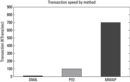
Figure 4.14 Performance of various transfer methods.
Exercises
P4.1. Suppose an application was profiled and it was discovered that the do_work function accounted for 50% of the execution time. If do_work was implemented in hardware, what is the largest speedup one could expect for the codesigned system?
P4.2. Consider the following snippet of a C program.
int x;
int y;
int div ( int m, int n ) {
if( n==2 ) y = m>>1;
else if( n==4 ) y = m>>2;
else y = m/n;
return y;
}
void sub1 ( int a, int b ) {
int t1, t2;
t1 = a−b;
t2 = a+b;
x = div(t1,t2);
}
(a) If div was determined to be a feature implemented in hardware, what is the affected, trapped state when it is invoked?
(b) Suppose div was merged into sub1 and together, implemented in as a hardware feature. Does it change the affected, trapped state?
P4.3. Consider subroutine fmul below.
float fmul ( float a, float b ) {
return a*b;
}
Give a practical explanation of why fmul might not be considered a candidate feature.
P4.4. Suppose subroutine crc below is a candidate feature,
int crc ( int input ) {
return ….;
}
Name three quantitative reasons it may not end up mapped to hardware.
P4.5. A software reference design has one main loop that takes 600 seconds to complete. The loop was executed on the target processor and each subroutine was timed. Table 4.1 shows this data. Each subroutine is called once and ![]() is the time it takes in seconds. The time to perform the same functions in hardware and the marshaling costs (in seconds) are also shown in the table. The resource usage of CLBs, BRAMs, and DSP blocks are also shown.
is the time it takes in seconds. The time to perform the same functions in hardware and the marshaling costs (in seconds) are also shown in the table. The resource usage of CLBs, BRAMs, and DSP blocks are also shown.
(a) Calculate the expected performance gains, ![]() , and rank the subroutines.
, and rank the subroutines.
(b) If all four subroutines are implemented in hardware, what is the overall expected improvement in speed, ![]() ?
?
(c) Ignoring routing concerns and assuming the target device has
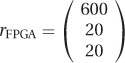
resources, what hardware/software partition yields the maximum speedup?
Table 4.1
Profile information for item 5.
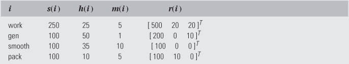
P4.6. Suppose a scientific application was profiled using gprof. The data for the top fifteen functions was collected and is shown in Table 4.2. (You may want to consult with gprof manual page to answer these questions.)
(a) Approximately how long did this application run?
(b) What is the difference between “self ms/call” and “total ms/call”? If these numbers are identical, what does this suggest?
(c) Suppose amp1 can be implemented in deeply pipelined core that takes 220 clock cycles to complete. It takes an additional 40 clock cycles to copy the data in and another 40 clock cycles to copy the data out. If the frequency is 100 MHz, what is the expected gain if amp1 is implemented in hardware?
(d) Suppose the same hardware function can be used to accelerate amp1, amp2, and amp3? What would be the overall expected system gain?
Table 4.2
Flat profile information for item 6.
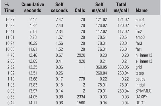
P4.7. Subroutine C consumes 85% of the execution time of an application. However, an engineer refactored the application so that a portion of subroutine C is moved into a new subroutine, C1 and then subroutine C calls C1. In this arrangement, subroutine, C1 accounts for only 80% of the execution time. C1 is mapped to hardware. How does a change like this impact expected system gain?
P4.8. Suppose the performance metric of interest was to cost savings so long as a minimum execution rate was met.
(a) How does this effect the formal framework presented in Section 5.2?
(c) Describe a heuristic to replace the one described in this chapter to maximize this performance metric (i.e. minimize cost).
P4.9. Suppose the performance metric of interest was energy consumption.
(a) What information is relevant at profiling to build a performance gain metric?
(b) Rework the performance gain metrics ![]() and
and ![]() with this information.
with this information.
(c) Will the heuristic described in this chapter be appropriate?
References
1. Adams MD. The jasper project home page 2007; http://www.ece.uvic.ca/mdadams/jasper/; 2007; last accessed May 2010.
2. Corbet J, Rubini A, Kroah-Hartman G. Linux device drivers 3rd ed. Sebastopol, CA, USA: O’Reilly & Associates, Inc. 2005; URL http://lwn.net/Kernel/LDD3; 2005.
3. Denning PJ, Kahn KC. A study of program locality and lifetime functions. In: SOSP ’75: Proceedings of the Fifth ACM Symposium on Operating Systems Principles. New York, NY, USA: ACM Press; 1975;207–216.
4. Graham SL, Kessler PB, McKusick MK. Gprof: A call graph execution profiler. In: SIGPLAN ’82: Proceedings of the 1982 SIGPLAN Symposium on Compiler Construction. New York, NY, USA: ACM; 1982;120–126.
1We are using a C++ shortcut here; alternatively int *x and (*x) could be substituted for int &x and x in the body.