Chapter 9
Sizing Software Deliverables

Up until this point our discussion of software cost estimating has dealt primarily with surface issues that are not highly complex. We are now beginning to deal with some of the software cost-estimating issues that are very complex indeed.

It will soon be evident why software cost-estimating tools either must be limited to a small range of software projects or else must utilize hundreds of rules and a knowledge base of thousands of projects in order to work well.

It is easier to build software estimating tools that aim at specific domains, such as those aimed only at military projects or at management information systems projects, than to build estimating tools that can work equally well with information systems, military software, systems and embedded software, commercial software, web applets, object-oriented applications, and the myriad of classes and types that comprise the overall software universe.

In this section we will begin to delve into some of the harder problems of software cost estimating that the vendors in the software cost-estimating business attempt to solve, and then we will place the solutions into our commercial software cost-estimating tools.

General Sizing Logic for Key Deliverables

One of the first and most important aspects of software cost estimating is that of sizing, or predicting the volumes of various kinds of software deliverable items. Sizing is a very complex problem for software cost estimating, but advances in sizing technology over the past 30 years have been impressive.

Software cost-estimating tools usually approach sizing in a sequential or cascade fashion. First, the overall size of the application is determined, using source code volumes, function point totals, use cases, stories, object points, screens, or some other metric of choice. Then the sizes for other kinds of artifacts and deliverable items are predicted based on the primary size in terms of LOC, function points, or whatever metric was selected.

TABLE 9.1 Software Artifacts for Which Size Information Is Useful

Before discussing how sizing is performed, it is useful to consider some 30 examples of the kinds of software artifacts for which sizing may be required. The main software artifacts are shown in Table 9.1.

Although this list is fairly extensive, it covers only the more obvious software artifacts that need to be dealt with. Let us now consider the sizing implications of these various software artifacts at a somewhat more detailed level.

Sizing Methods Circa 2007

One of the major historical problems of the software engineering world has been the need to attempt to produce accurate cost estimates for software projects before the requirements are fully known.

The first step in software cost estimating requires a knowledge of the size of the application in some tangible measurement such as lines of code, function points, object points, use cases, story points, or some other alternative.

The eventual size of the application is, of course, derived from user requirements of the application. Thus sizing and understanding user requirements are essentially the same problem.

Empirical data from hundreds of measured software projects reveals that a full and perfect understanding of user requirements is not usually possible to achieve at one time. User requirements tend to unfold and grow over time. In fact, the measured rate of this growth of user requirements averages 2 percent per calendar month, from the end of the nominal “requirements phase” through the subsequent design and coding phases.

The total accumulated growth in requirements averages about 25 percent more than initially envisioned, but the maximum growth in requirements has exceeded 100 percent. That is, the final application ends up being about twice as large as initially envisioned.

Historically, the growth in requirements after the formal requirements phase has led to several different approaches for dealing with this phenomenon, such as the following:

Improved methods of requirements gathering such as joint application design (JAD), where clients work side by side with designers using formal methods that are intended to gather requirements with few omissions.

Freezing requirements for the initial release at some arbitrary point. Additional requirements are moved into subsequent releases.

Including anticipated growth in the initial cost estimates. Often the first estimate will include an arbitrary “contingency factor” such as an additional 35 percent for handling unknown future requirements that occur after the estimate is produced.

Various forms of iterative development, where pieces of the final application are developed and used before starting to build the next set of features.

Various forms of Agile development, where development commences when only the most important and obvious features are understood. As experiences with using the first features accumulate, additional features are planned and constructed. The features for the final application may not be understood until a number of versions have been developed and used. For some of the Agile approaches, clients are part of the team and so the requirements evolve in real time.

Software applications are a different kind of engineering problem from designing a house or a tangible object such as an automobile. Before construction starts on a house, a full set of design blueprints are developed by the architect, using inputs from the owners. It does happen that the owners may make changes afterwards, but usually the initial blueprint is more than 95 percent complete.

Unfortunately for the software world, clients usually demand cost estimates for 100 percent of the final application at a point in time where less than 50 percent of the final features are understood. A key challenge to software estimating specialists and software project managers is to find effective methods for sizing applications in the absence of full knowledge of their final requirements.

Some of the methods that have developed for producing software application size and cost estimates in the absence of full requirements include the following:

Pattern matching, or using historical data from similar projects as the basis for both predicting the final size and costs of a new project.

Using historical data on the average rate of requirements growth to predict the probable amount of growth from the time of the first estimate to the end of the project.

Using various mathematical or statistical methods to attempt a final size prediction from partial requirements.

Using arbitrary rules of thumb to add “contingency” amounts to initial estimates to fund future requirements.

Attempting to limit requirements growth by freezing requirements at a specific point, and deferring all additions to future versions that will have their own separate cost estimates.

Producing formal cost estimates only for the features and requirements that are fully understood, and delaying the production of a full cost estimate until later when the requirements are finally defined.

Let us consider the pros and cons of these six methods for dealing with sizing software applications in the absence of full requirements.

Pattern Matching from Historical Data

In 2007, about 70 percent of all software applications are repeats of legacy applications that have lived past their prime and need to be retired. However, only about 15 percent of these legacy applications have reasonably complete historical data available in terms of schedules, costs, and quality. What the legacy applications do have available is a known size. However this size data may only be available in terms of source code. Also, the programming language for the legacy software is probably not going to be the same as that of the new replacement application.

For example, if you are replacing a legacy order entry system circa 1990 with a new application, the size of the legacy application might be 5000 function points and 135,000 COBOL source statements in size.

The new version will probably include all of the existing legacy features, and some new features as well. You might also be planning to use an object-oriented method of developing the new version and the Smalltalk programming language.

You can assume that the set of features for the new application will be larger than the old but the source code volume might not be. Using the legacy application as the starting point, and some suitable conversion rules, you might predict that the new version will be about 6000 object points in size. The volume of code in the Smalltalk programming language might be about 36,000 Smalltalk statements since Smalltalk is a much more powerful language than COBOL.

As an additional assumption since you are using OO methods and code, you probably will have about 50 percent reusable code so you will only be developing about 3000 object points and 18,000 new Smalltalk statements.

Of course, this is not a perfect approach to sizing, but if you do happen to have historical size information available from one or more similar legacy applications, you can be reasonably sure that you will not under-state the size of the new application. The new application will almost certainly be somewhat larger than the old in terms of features.

If you have access to a large volume of historical data from a consulting company or benchmark group you might be able to evaluate a number of similar legacy applications. Doing this requires a benchmark database and a good taxonomy of application nature, class, scope, and type in order to ensure appropriate matches.

Pattern matching from legacy applications is the only method that can be used before requirements gathering is started. Thus, pattern matching provides the earliest chronology for creating a cost estimate that does not depend almost exclusively on guesswork.

Using Historical Data to Predict Growth in Requirements

It is a proven fact that for large software applications, the requirements are never fully defined at the end of the nominal requirements phase. It is also a proven fact that requirements typically grow at a rate of about 2 percent per calendar month assuming a standard waterfall development model and a normal requirements gathering and analysis process.

This growth continues during the subsequent design and coding phases, but stops at the testing phase. For an application with a six-month design phase and a nine-month coding phase, the cumulative growth will be about 30 percent in new features.

(However, if you are using one of the Agile methods that concentrates exclusively on the most obvious and important initial requirements, the monthly rate of growth in new requirements will be about 15 percent per calendar month. For an Agile application with a one-month design phase and four months of sprints or iterations, the cumulative growth in requirements will be about 75 percent in new features.)

Thus, historical data from past projects that show the rate at which requirements evolve and grow during the development cycle can be used to estimate the probable size of the entire application. Incidentally, predicting the growth of requirements over time is a useful adjunct to the method of “earned value” costing.

Several commercial software cost-estimating tools include features that attempt to predict the volume of growth of requirements after the requirements phase. The actual calculations, of course, are somewhat more complex than the simple examples discussed here.

Mathematical or Statistical Attempts to Extrapolate Size from Partial Requirements

Recall from Chapters 6, 7, and 8 that the taxonomy of nature, class, type, and scope places a software application squarely among similar applications. In fact, once an application has been placed in this taxonomy, simply raising the sum to the 2.35 power will yield a rough approximation of the function point total for the application as illustrated in Chapter 8. Similar rules can be applied to predict the number of object points, use case points, or other metrics.

One of the characteristics of applications that occupy the same place in a taxonomy is that such applications often have very similar distributions of function point values for the five elements: inputs, outputs, inquiries, logical files, and interfaces.

Assume that the taxonomy of your new application matches a legacy application that had 50 inputs, 75 outputs, 50 inquiries, 15 logical files, and 10 interfaces. When analyzing early requirements for the new application, you will probably start with “outputs” since that is the most common starting place for understanding user needs.

If you ascertain that your new application will have 80 outputs, then you have enough information to make a mathematical prediction of likely values for the missing data on inputs, inquiries, logical files, and interfaces. Thus, you can predict about 53 inputs, 80 outputs, 53 inquiries, 17 logical files, and 11 interfaces.

We started with knowledge only of the outputs, and used mathematical extrapolation to predict the missing values.

Similar kinds of predictions could also be made with object points or use case points. However, there is comparatively little historical data available that is expressed in terms of either object points or use case points.

Some commercial software cost-estimating tools do include extrapolation features from partial knowledge. It should be noted that there are two drawbacks to sizing using this approach: (1) you need firm knowledge of the size of at least one factor, and (2) you need access to historical data from similar projects.

Also, from time to time new applications will not actually match the volumes of inputs, outputs, inquiries, etc., from legacy or historical projects. Thus, this method occasionally will lead to erroneous sizing.

Arbitrary Rules of Thumb for Adding Contingency Factors

The oldest and simplest method for dealing with incomplete requirements is to add a contingency factor to each cost estimate. These contingency factors are usually expressed as simple percentages of the total cost estimate. For example, back in the 1970s IBM used the following sliding scale of contingency factors for software cost estimates:

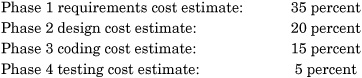
The rationale for these contingency factors is that the extra money would be used to fund requirements that had not been understood or present at the time of each cost estimate. In other words, although expressed in terms of dollars, contingency factors are inserted to deal with the growth of unknown requirements and to handle the increase in size that these requirements will cause.

While the contingency factors were moderately successful in the 1970s, they gradually ran into technical difficulties. As typical IBM applications grew in size from less than 1000 function points in the 1970s to more than 10,000 function points in the 1990s, the contingency factors needed to be increased. This is because for large systems, less is known early and more growth occurs later on.

To use simple percentage contingency factors on applications in the 10,000–function point range, the values would have to approximate the following:

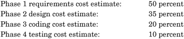
However, such large contingency factors are psychologically unsettling to executives and clients. They feel uncomfortable with estimates that are based on such large adjustment factors.

Freezing Requirements at Fixed Points in Time

Since the 1970s some large corporations such as AT&T, IBM, and Microsoft have had firm cut-off dates for all features that were intended to go out in a specific releases. After the initial release of a large system such as the AT&T ESS5 switching system, IBM’s MVS operating system, and Microsoft’s Windows XP operating system, future releases are planned at fixed intervals.

For example, IBM would plan a maintenance release for bug repairs six months after the initial release of an application, and then add new features 12 months after the initial release. Maintenance releases and new-feature releases would then continue to alternate on those schedules for about five calendar years. After about 36 months there would be a “mid-life kicker” or a release with quite a lot of interesting new features.

New features would be targeted for a specific release, but if there were problems that made a feature miss its planned release, it had to wait for another 12 months before going out. This sometimes led to rushing and poor quality in order to meet the deadline for an important new feature.

It also happens that for very large systems in the 10,000–function point range (equivalent to 500,000 Java statements or 1,250,000 C statements) the initial release usually contains only about 80 percent of the features that were originally intended. An analysis of large IBM applications by the author in the 1970s found that 20 percent of planned features missed the first release. However, about 30 percent of the features in the first release were not originally planned, but occurred later in the form of creeping requirements. This is a fairly typical pattern.

For large applications that are likely to last for five or ten years once deployed, having fixed release intervals is a fairly effective solution. Development teams soon become comfortable with fixed release intervals and can plan accordingly.

Also, customers or clients usually prefer a fixed release interval because it makes their maintenance and support planning easier and helps keep costs level over time. The one exception to the advantages of fixed release intervals is the case of high-severity defects, which need to be fixed and released as quickly as possible.

For example, users of Microsoft Windows receive very frequent updates from Microsoft when security breaches or other critical problems are found in Windows XP or Microsoft Office.

Producing Formal Cost Estimates Only for Subsets of the Total Application

Some of the Agile approaches attempt to avoid the problems of complete sizing and cost estimating in the absence of full requirements by producing cost estimates only for the next iteration or sprint that will be produced. The overall or final cost for the application is not attempted, on the grounds that it is probably unknowable until customers have used the early releases and decided what they want next.

This method does avoid large errors in sizing and cost estimating. But that is because the predictions of the final size and final costs are not attempted initially. Currently in 2007, this approach is used mainly for internal projects where the costs and schedule are not subject to contractual requirements. It is not currently the method of choice for fixed-price contracts or for other software applications where the total cost must be known for legal or corporate reasons.

The approach of formal estimates only for the next sprint or iteration does fit in reasonably well with the “earned value” approach, although not very many Agile projects have reported using earned value measurements to date.

However, as more and more Agile projects are completed there will be a steady accumulation of historical data. Within a few years, there should be enough information to know the total numbers of stories, story points, use cases, sprints, and other data from hundreds of Agile projects.

Within perhaps five or ten years, pattern matching approaches will begin to be widely available in an Agile context. Once there is a critical mass of completed Agile projects with historical data available, then it will be possible to use this information to predict overall sizes and costs for new applications.

This means that the Agile development teams will have to record historical information, which will add slightly to the effort for developing the applications.

The same kinds of patterns are starting to be developed for object-oriented projects. At some point in the near future, pattern matching will begin to be effective not only for the technical features of OO applications, but also for predicting costs, schedules, staffing, quality, and other business features as well.

Function Point Variations Circa 2007

Over and above the function point metric defined by IFPUG, there are close to 40 other variants that do not give the same results as the IFPUG method. Further, many of the function point variants have no published conversion rules to standard IFPUG function points or much data of any kind in print.

This means that the same application can appear to have very different sizes, based on whether the function point totals follow the IFPUG counting rules, the British Mark II counting rules, COSMIC function point counting rules, object-point counting rules, the SPR feature point counting rules, the Boeing 3D counting rules, or any of the other function point variants. Thus, application sizing and cost estimating based on function point metrics must also identify the rules and definitions of the specific form of function point being utilized.

These variants have introduced serious technical challenges into software benchmarks and economic analysis. Suppose you were a metrics consultant with a client in the telecommunications industry who wanted to know what methods and programming languages gave the best productivity for PBX switching systems. This is a fairly common kind of request.

You search various benchmark data bases and find 21 PBX switching systems that appear to be relevant to the client’s request. Now the problems start:

Three of the PBXs were measured using “lines of code.” One counted physical lines, one counted logical statements, and one did not define which method was used.

Three of the PBXs were object-oriented. One was counted using object points and two were counted with use case points.

Three of the PBXs were counted with IFPUG function points.

Three of the PBXs were counted with COSMIC function points.

Three of the PBXs were counted with NESMA function points.

Three of the PBXs were counted with Feature points.

Three of the PBXs were counted with Mark II function points

As of 2007, there is no easy technical way to provide the client with an accurate answer to what is really a basic economic question. You cannot average the results of these 21 similar projects nor do any kind of useful statistical analysis because of the use of so many different metrics.

Prior to this book there have been no published conversion rules from one metric variant to another. Although this book does have some tentative conversion rules, they are not viewed by the author as being accurate enough to use for serious business purposes such as providing clients with valid comparisons between projects counted via different approaches.

In the author’s opinion, the developers of alternate function point metrics have a professional obligation to provide conversion rules from their new metrics to the older IFPUG function point metric. It is not the job of IFPUG to evaluation every new alternative.

Also, IFPUG itself introduced a major change in function point counting rules in 1994, when Version 4 of the rules was published. The Version 4 changes eliminated counts of some forms of error messages (over substantial protest, it should be noted) and, hence, reduced the counts from the prior Version 3.4 by perhaps 20 percent for projects with significant numbers of error messages.

The function point sizes in this book are based on IFPUG counts, with Version 4.1 being the most commonly used variant. However, from time to time points require that the older Version 3.4 form be used. The text will indicate which form is utilized for specific cases.

Over and above the need to be very clear as to which specific function point is being used, there are also some other issues associated with function point sizing that need to be considered.

The rules for counting function points using most of the common function point variants are rather complex. This means that attempts to count function points by untrained individuals generally lead to major errors. This is unfortunate, but is also true of almost any other significant metric.

Both the IFPUG and the equivalent organization in the United Kingdom, the United Kingdom Function Point (Mark II) Users Group, offer training and certification examinations. Other metrics organizations, such as the Australian Software Metrics Association (ASMA) and the Netherlands Software Metrics Association (NESMA) may also offer certification services. However, most of the minor function point variants have no certification examinations and have very little published data.

When reviewing data expressed in function points, it is important to know whether the published function point totals used for software cost estimates are derived from counts by certified function point counters, from attempts to create totals by untrained counters, or from four other common ways of deriving function point totals:

Backfiring from source code counts, either manually or using tools such as those marketed by ViaSoft

Automatic generation of function points from requirements and design, using tools

Deriving function points by analogy, such as assuming that Project B will be the same size as Project A, a prior project that has a function point size of known value

Counting function points using one of the many variations in functional counting methods (i.e., SPR feature points, Boeing 3D function points, COSMIC function points, Netherlands function points, etc.)

(Of course it is also important to know whether data expressed in lines of code is based on counts of physical lines or logical statements, just as it is important to know whether distance data expressed in miles refers to statute miles or nautical miles, or whether volumetric data expressed in terms of gallons refers to U.S. gallons or Imperial gallons.)

As a result of the lack of written information for legacy projects, the method called “backfiring,” or direct conversion from source code statements to equivalent function point totals, has become one of the most widely used methods for determining the function point totals of legacy applications. Since legacy applications far outnumber new software projects, this means that backfiring is actually the most widely used method for deriving function point totals.

Backfiring is highly automated, and a number of vendors provide tools that can convert source code statements into equivalent function point values. Backfiring is very easy to perform, so that the function point totals for applications as large as 1 million source code statements can be derived in only a few minutes of computer time.

The downside of backfiring is that it is based on highly variable relationships between source code volumes and function point totals. Although backfiring may achieve statistically useful results when averaged over hundreds of projects, it may not be accurate by even plus or minus 50 percent for any specific project. This is due to the fact that individual programming styles can create very different volumes of source code for the same feature. Controlled experiments by IBM in which eight programmers coded the same specification found variations of about 5 to 1 in the volume of source code written by the participants.

Also, backfiring results will vary widely based upon whether the starting point is a count of physical lines, or a count of logical statements. In general, starting with logical statements will give more accurate results. However, counts of logical statements are harder to find than counts of physical lines.

In spite of the uncertainty of backfiring, it is supported by more tools and is a feature of more commercial software estimating tools than any other current sizing method. The need for speed and low sizing costs explains why many of the approximation methods, such as backfiring, sizing by analogy, and automated function point derivations, are so popular: They are fast and cheap, even if they are not as accurate. It also explains why so many software-tool vendors are actively exploring automated rule-based function point sizing engines that can derive function point totals from requirements and specifications, with little or no human involvement.

Since function point metrics have splintered in recent years, the family of possible function point variants used for estimation and measurement include at least 38 choices (see Table 9.2).

Note that this listing is not stated to be 100 percent complete. The 38 variants shown in Table 9.2 are merely the ones that have surfaced in the software measurement literature or been discussed at metrics conferences. No doubt, at least another 20 or so variants may exist that have not yet published any information or been presented at metrics conferences.

TABLE 9.2 Function Point Counting Variations Circa 2007

With some reluctance, the author is providing a table of conversion factors between some of the more common function point variants and standard IFPUG function points (see Table 9.3). The accuracy of the conversion ratios is questionable in 2007. Hopefully, even the publication of incorrect conversion rules will lead to refinements and more accurate rules in the future. This is an area that needs a great deal of research.

TABLE 9.3 Approximate Conversion Ratios to IFPUG Function Points (Assumes Version 4.1 of the IFPUG Counting Rules)

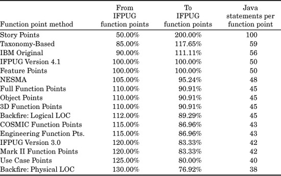
Table 9.3 uses IFPUG 4.1 as its base. If you want to convert 100 IFPUG function points to COSMIC function points, use the “From IFPUG...” column. The result would be about 115 COSMIC function points. Going the other way, if you start with 100 COSMIC function points and want to convert to IFPUG, use the “To IFPUG...” column. The result would be about 87 IFPUG function points.

If you want to perform conversions among the other metrics, you will need to do a double conversion. For example, if you want to convert use case points into COSMIC function points, you will have to convert both values into IFPUG first. If you start with 100 use case points, that is equal to about 80 IFPUG function points. Then you would use the “From IFPUG...” value of 115 percent for COSMIC, and the result would be about 92 COSMIC function points.

The software industry has long been criticized for lacking good historical data and for inaccurate sizing and estimating of many applications. Unfortunately, the existence of so many different metrics is exacerbating an already difficult challenge for software estimators.

Reasons Cited for Creating Function Point Variations

The reasons why there are at least 38 variations in counting function points deserve some research and discussion. First, it was proven long ago in the 1970s that the lines-of-code-metrics cannot measure software productivity in an economic sense and is harmful for activity-based cost analysis. Therefore, there is a strong incentive to adopt some form of functional metric because the older LOC method has been proven to be unreliable.

However, the mushrooming growth of function point variations can be traced to other causes. From meetings and discussions with the developers of many function point variants, the following reasons have been noted as to why variations have been created.

First, a significant number of variations were created due to a misinterpretation of the nature of function point metrics. Because the original IBM function points were first applied to information systems, a belief grew up that standard function points don’t work for real-time and embedded software. This belief is caused by the fact that productivity rates for real-time and embedded software are usually well below the rates for information systems of the same size measured with function points.

Almost all of the function point variants yield larger counts for real-time and embedded software than do standard IFPUG function points.

The main factors identified as differentiating embedded and real-time software from information systems applications include the following:

Embedded software is high in algorithmic complexity.

Embedded software is often limited in logical files.

Embedded software’s inputs and outputs may be electronic signals.

Embedded software’s interfaces may be electronic signals.

The user view for embedded software may not reflect human users.

These differences are great enough that the real-time and systems community has been motivated to create a number of function point variations that give more weight to algorithms, give less weight to logical files, and expand the concept of inputs and outputs to deal with electronic signals and sensor-based data rather than human-oriented inputs and outputs, such as forms and screens. Are these alternative function point methods really useful? There is no definitive answer, but from the point of view of benchmarking and international comparisons they have caused more harm than they have created value.

Another phenomenon noted when exploring function point variations is the fact that many function point variants are aligned to national borders. The IFPUG is headquartered in the United States, and most of the current officers and committee chairs are U.S. citizens.

There is a widespread feeling in Europe and elsewhere that in spite of the association having international in its name, IFPUG is dominated by the United States and may not properly reflect the interests of Europe, South America, the Pacific Rim, or Australia. Therefore, some of the function point variants are more or less bounded by national borders, such as the Netherlands function point method and the older British Mark II function point method.

If function points are to remain viable into the next century, it is urgent to focus energies on perfecting one primary form of functional metric rather than dissipating energies into the creation of scores of minor function point variants, many of which have no published data and have only a handful of users.

Even worse, while many months of effort have been spent developing 38 function point variants, some major measurement and metrics issues are almost totally unexamined. As will be pointed out later in this chapter, the software engineering community lags physics and engineering in understanding and measuring complexity. Also, there are no effective measurements for database volumes or database quality. There are no effective measurements or metrics that can deal with intangible value. There are no good measurements or metrics for customer service. It would be far more useful for software engineering if metrics research began to concentrate on important topics that are beyond the current measurement state of the art, rather than dissipating energies on scores of minor function point variants.

Regardless of the reasons, the existence of so many variations in counting function points is damaging to the overall software metrics community and is not really advancing the state of the art of software measurement.

As the situation currently stands, the overall range of apparent function point counts for the same application can vary by perhaps two to one, based on which specific varieties of function point metrics are utilized. This situation obviously requires that the specific form of function point be recorded in order for the size information to have any value.

Although the large range of metric choices all using the name “function points” is a troublesome situation, it is not unique to software. Other measurements outside the software arena also have multiple choices for metrics that use the same name. For example, it is necessary to know whether statute miles or nautical miles are being used; whether American dollars, Australian dollars, or Canadian dollars are being used; and whether American gallons or Imperial gallons are being used. It is also necessary to know whether temperatures are being measured in Celsius or Fahrenheit degrees. There are also three ways of calculating the octane rating of fuel, and several competing methods for calculating fuel efficiency or miles per gallon. There are even multiple ways of calculating birthdays.

However, the explosion of the function point metric into 38 or so competitive claimants must be viewed as an excessive number of choices. Hopefully, the situation will not reach the point seen among programming languages, where 600 or more languages are competing for market share.

Volume of Function Point Data Available

The next table is an attempt to quantify the approximate number of software projects that have been measured using various forms of metrics. IFPUG Version 4.1 is in the majority, but due to the global preponderance of aging legacy applications, various forms of backfiring appear to be the major sources of global function point data for maintenance projects.

The information in Table 9.4 is derived from discussions with various benchmarking companies, from the software metrics literature, and from informal discussions with function point users and developers during the course of software assessment and benchmarking studies. The table has a high margin of error and is simply a rough attempt to evaluate the size of the universe of function point data and lines of code data when all major variations are included.

TABLE 9.4: Approximate Numbers of Projects Measured

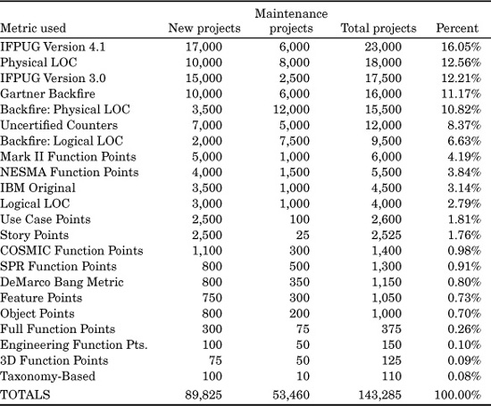
Because aging legacy applications comprise the bulk of all software projects in the world, the various forms of backfiring, or direct conversion between source code statements and function points, is the most widely utilized method for enumerating function points, especially for legacy applications. All of the major software benchmarking companies (e.g., Davids, Gartner Group, SPR, etc.) utilize backfiring for their client studies and, hence, have substantial data derived from backfiring.

Curiously, none of the major function point groups, such as IFPUG, the United Kingdom Function Point Users Group, or the Netherlands Software Metrics Association, have attempted any formal studies of backfiring, or even made any visible contribution to this popular technology. The great majority of reports and data on backfiring come from the commercial benchmark consulting companies, such as the David’s Consulting Company, Gartner Group, Rubin Systems, and Software Productivity Research.

As stated, the margin of error with Table 9.4 is very high, and the information is derived from informal surveys at various function point events in the United States, Europe, and the Pacific Rim. However, there seems to be no other source of this kind of information on the distribution of software projects among the various forms of function point analysis.

It is also curious that none of the function point user associations, such as IFPUG or the United Kingdom Function Point Users Group, have attempted to quantify the world number of projects measured using function points. IFPUG has attempted some benchmarking work, but only in the context of projects measured using the IFPUG Version 4 counting rules.

Unfortunately, the major function point associations, such as IFPUG in the United States, the British Mark II users group, NESMA, ASMA, and others, tend to view each other as political rivals and, hence, ignore one another’s data or sometimes even actively disparage one another.

Consider yet another issue associated with function point metrics. The minimum weighting factors assigned to standard IFPUG function points have a lower limit or cut-off point. These limits mean that the smallest practical project where such common function point metrics as IFPUG and Mark II can be used is in the vicinity of 10 to 15 function points. Below that size, the weighting factors tend to negate the use of the function point metric.

Because of the large number of small maintenance and enhancement projects, there is a need for some kind of micro–function point that can be used in the zone that runs from a fraction of a single function point up to the current minimum level where normal function points apply.

Since it is the weighting factors that cause the problem with small projects, one obvious approach would be to use unadjusted function point counts for small projects without applying any weights at all. However, this experimental solution would necessitate changes in the logic of software estimating tools to accommodate this variation.

The huge numbers of possible methods for counting function points are very troublesome for software cost-estimating tool vendors and for all those who build metrics tools and software project management tools. None of us can support all 38 variations in function point counting, so most of us support only a subset of the major methods.

Software Complexity Analysis

The topic of complexity is very important for software cost estimation because it affects a number of independent and dependent variables, such as the following:

High complexity levels can increase bug or defect rates.

High complexity levels can lower defect-removal efficiency rates.

High complexity levels can decrease development productivity rates.

High complexity levels can raise maintenance staffing needs.

High complexity levels can lengthen development schedules.

High complexity levels increase the number of test cases needed.

High complexity levels affect the size of the software application.

High complexity levels change backfiring ratios.

Unfortunately, the concept of complexity is an ambiguous topic that has no exact definition agreed upon by all software researchers. When we speak of complexity in a software context, we can be discussing the difficulty of the problem that the software application will attempt to implement, the structure of the code, or the relationships among the data items that will be used by the application. In other words, the term complexity can be used in a general way to discuss problem complexity, code complexity, and data complexity.

The scientific and engineering literature encompasses no fewer than 30 different flavors of complexity, some or all of which may be found to be relevant for software applications. Unfortunately, most of the forms of scientific complexity are not even utilized in a software context. The software engineering community is far behind physics and other forms of engineering in measuring and understanding complexity.

In a very large book on software complexity, Dr. Horst Zuse (Software Complexity: Measures and Methods; Walter de Gruyter, Berlin 1990) discusses about 50 variants of structural complexity for programming alone. It is perhaps because of the European origin—functional metrics are not as dominant there as in the United States—but in spite of the book’s large size and fairly complete treatment, Zuse seems to omit all references to function point metrics and to the forms of complexity associated with functional metrics.

When software sizing and estimating tools utilize complexity as an adjustment factor, the methods tend to be highly subjective. Some of the varieties of complexity encountered in the scientific literature that show up in a software context include the following:

Algorithmic complexity concerns the length and structure of the algorithms for computable problems. Software applications with long and convoluted algorithms are difficult to design, to inspect, to code, to prove, to debug, and to test. Although algorithmic complexity affects quality, development productivity, and maintenance productivity, it is utilized as an explicit factor by only a few software cost-estimating tools.

Code complexity concerns the subjective views of development and maintenance personnel about whether the code they are responsible for is complex or not. Interviewing software personnel and collecting their subjective opinions is an important step in calibrating more formal complexity metrics, such as cyclomatic and essential complexity. A number of software estimating tools have methods for entering and adjusting code complexity based on ranking tables that run from high to low complexity in the subjective view of the developers.

Combinatorial complexity concerns the numbers of subsets and sets that can be constructed out of N components. This concept sometimes shows up in the way that modules and components of software applications might be structured. From a psychological vantage point, combinatorial complexity is a key reason why some problems seem harder to solve than others. However, this form of complexity is not utilized as an explicit estimating parameter.

Computational complexity concerns the amount of machine time and the number of iterations required to execute an algorithm. Some problems are so high in computational complexity that they are considered to be noncomputable. Other problems are solvable but require enormous quantities of machine time, such as cryptanalysis or meteorological analysis of weather patterns. Computational complexity is sometimes used for evaluating the performance implications of software applications, but not the difficulty of building or maintaining them.

Cyclomatic complexity is derived from graph theory and was made popular for software by Dr. Tom McCabe (IEEE Transactions on Software Engineering, Vol SE2, No. 4 1976). Cyclomatic complexity is a measure of the control flow of a graph of the structure of a piece of software. The general formula for calculating cyclomatic complexity of a control flow graph is edges − nodes + unconnected parts × 2. Software with no branches has a cyclomatic complexity level of 1. As branches increase in number, cyclomatic complexity levels also rise. Above a cyclomatic complexity level of 20, path flow testing becomes difficult and, for higher levels, probably impossible.

Cyclomatic complexity is often used as a warning indicator for potential quality problems. Cyclomatic complexity is the most common form of complexity analysis for software projects and the only one with an extensive literature. At least 20 tools can measure cyclomatic complexity, and these tools range from freeware to commercial products. Such tools support many programming languages and operate on a variety of platforms.

Data complexity deals with the number of attributes associated with entities. For example, some of the attributes that might be associated with a human being in a typical medical office database of patient records could include date of birth, sex, marital status, children, brothers and sisters, height, weight, missing limbs, and many others. Data complexity is a key factor in dealing with data quality. Unfortunately, there is no metric for evaluating data complexity, so only subjective ranges are used for estimating purposes.

Diagnostic complexity is derived from medical practice, where it deals with the combinations of symptoms (temperature, blood pressure, lesions, etc.) needed to identify an illness unambiguously. For example, for many years it was not easy to tell whether a patient had tuberculosis or histoplasmosis because the superficial symptoms were essentially the same. For software, diagnostic complexity comes into play when customers report defects and the vendor tries to isolate the relevant symptoms and figure out what is really wrong. However, diagnostic complexity is not used as an estimating parameter for software projects.

Entropic complexity is the state of disorder of the component parts of a system. Entropy is an important concept because all known systems have an increase in entropy over time. That is, disorder gradually increases. This phenomenon has been observed to occur with software projects because many small changes over time gradually erode the original structure. Long-range studies of software projects in maintenance mode attempt to measure the rate at which entropy increases and determine whether it can be reversed by such approaches as code restructuring. Surrogate metrics for evaluating entropic complexity are the rates at which cyclomatic and essential complexity change over time, such as on an annual basis. However, there are no direct measures for software entropy.

Essential complexity is also derived from graph theory and was made popular by Dr. Tom McCabe (IEEE Transactions on Software Engineering, Vol SE2, No. 4 1976). The essential complexity of a piece of software is derived from cyclomatic complexity after the graph of the application has been simplified by removing redundant paths. Essential complexity is often used as a warning indicator for potential quality problems. As with cyclomatic complexity, a module with no branches at all has an essential complexity level of 1. As unique branching sequences increase in number, both cyclomatic and essential complexity levels will rise. Essential complexity and cyclomatic complexity are supported by a variety of software tools.

Fan complexity refers to the number of times a software module is called (termed fan in) or the number of modules that it calls (termed fan out). Modules with a large fan-in number are obviously critical in terms of software quality, since they are called by many other modules. However, modules with a large fan-out number are also important, and they are hard to debug because they depend upon so many extraneous modules. Fan complexity is relevant to exploration of reuse potentials. Fan complexity is not used as an explicit estimating parameter, although in real life this form of complexity appears to exert a significant impact on software quality.

Flow complexity is a major topic in the studies of fluid dynamics and meteorology. It deals with the turbulence of fluids moving through channels and across obstacles. A new subdomain of mathematical physics called chaos theory has elevated the importance of flow complexity for dealing with physical problems. Many of the concepts, including chaos theory itself, appear relevant to software and are starting to be explored. However, the application of flow complexity to software is still highly experimental.

Function point complexity refers to the set of adjustment factors needed to calculate the final adjusted function point total of a software project. Standard U.S. function points as defined by the IFPUG have 14 complexity adjustment factors. The British Mark II function point uses 19 complexity adjustment factors. The SPR function point and feature point metrics use three complexity adjustment factors. Function point complexity is usually calculated by reference to tables of known values, many of which are automated and are present in software estimating tools or function point analysis tools.

Graph complexity is derived from graph theory and deals with the numbers of edges and nodes on graphs created for various purposes. The concept is significant for software because it is part of the analysis of cyclomatic and essential complexity, and also is part of the operation of several source code restructuring tools. Although derivative metrics, such as cyclomatic and essential complexity, are used in software estimating, graph theory itself is not utilized.

Halstead complexity is derived from the software-science research carried out by the late Dr. Maurice Halstead (Elements of Software Science, Elsevier North Holland, New York, 1977) and his colleagues and students at Purdue University. The Halstead software science treatment of complexity is based on four discrete units: (1) number of unique operators (i.e., verbs), (2) number of unique operands (i.e., nouns), (3) instances of operator occurrences, and (4) instances of operand occurrences.

The Halstead work overlaps linguistic research, in that it seeks to enumerate such concepts as the vocabulary of a software project. Although the Halstead software-science metrics are supported in some software cost-estimating tools, there is very little recent literature on this topic.

Information complexity is concerned with the numbers of entities and the relationships between them that might be found in a database, data repository, or data warehouse. Informational complexity is also associated with research on data quality. Unfortunately, all forms of research into database sizes and database quality are handicapped by the lack of metrics for dealing with data size, or for quantifying the forms of complexity that are likely to be troublesome in a database context.

Logical complexity is important for both software and circuit design. It is based upon the combinations of AND, OR, NOR, and NAND logic conditions that are concatenated together. This form of complexity is significant for expressing algorithms and for proofs of correctness. However, logical complexity is utilized as an explicit estimating parameter in only a few software cost-estimating tools.

Mnemonic complexity is derived from cognitive psychology and deals with the ease or difficulty of memorization. It is well known that the human mind has both temporary and permanent memory. Some kinds of information (i.e., names and telephone numbers) are held in temporary memory and require conscious effort to be moved into permanent memory. Other kinds of information (i.e., smells and faces) go directly to permanent memory.

Mnemonic complexity is important for software debugging and during design and code inspections. Many procedural programming languages have symbolic conventions that are very difficult to either scan or debug because they oversaturate human temporary memory. Things such as nested loops that use multiple levels of parentheses—that is, (((...)))—tend to swamp human temporary memory capacity.

Mnemonic complexity appears to be a factor in learning and using programming languages, and is also associated with defect rates in various languages. However, little information is available on this potentially important topic in a software context, and it is not used as an explicit software estimating parameter.

Organizational complexity deals with the way human beings in corporations arrange themselves into hierarchical groups or matrix organizations. This topic might be assumed to have only an indirect bearing on software, except for the fact that many large software projects are decomposed into components that fit the current organizational structure rather than the technical needs of the project. For example, many large software projects are decomposed into segments that can be handled by eight-person departments, whether or not that approach meets the needs of the system’s architecture.

Although organizational complexity is seldom utilized as an explicit estimating parameter, it is known that large software projects that are well organized will outperform similar projects with poor organizational structures.

Perceptional complexity is derived from cognitive psychology and deals with the arrangements of edges and surfaces that appear to be simple or complex to human observers. For example, regular patterns appear to be simple while random arrangements appear to be complex. This topic is important for studies of visualization, software design methods, and evaluation of screen readability. Unfortunately, the important topic of the perceptional complexity of various software design graphics has only a few citations in the literature, and none in the cost-estimating literature.

Problem complexity concerns the subjective views of people asked to solve various kinds of problems about their difficulty. Psychologists know that increasing the number of variables and the length of the chain of deductive reasoning usually brings about an increase in the subjective view that the problem is complex. Inductive reasoning also adds to the perception of complexity. In a software context, problem complexity is concerned with the algorithms that will become part of a program or system. Determining the subjective opinions of real people is a necessary step in calibrating more objective complexity measures.

Process complexity is mathematically related to flow complexity, but in day-to-day software work it is concerned with the flow of materials through a software development cycle. This aspect of complexity is often dealt with in a practical way by project management tools that can calculate critical paths and program evaluation and review technique (PERT) diagrams of software development processes.

Semantic complexity is derived from the study of linguistics and is concerned with ambiguities in the definitions of terms. Already cited in this book are the very ambiguous terms quality, data, and complexity. The topic of semantic complexity is relevant to software for a surprising reason: Many lawsuits between software developers and their clients can be traced back to the semantic complexity of the contract when both sides claim different interpretations of the same clauses. Semantic complexity is not used as a formal estimating parameter.

Syntactic complexity is also derived from linguistics and deals with the grammatical structure and lengths of prose sections, such as sentences and paragraphs. A variety of commercial software tools are available for measuring syntactic complexity, using such metrics as the FOG index. (Unfortunately, these tools are seldom applied to software specifications, although they would appear to be valuable for that purpose.)

Topologic complexity deals with rotation and folding patterns. This topic is often explored by mathematicians, but it also has relevance for software. For example, topological complexity is a factor in some of the commercial source code restructuring tools.

As can be seen from the variety of subjects included under the blanket term complexity, this is not an easy topic to deal with. From the standpoint of sizing software projects, 6 of the 24 flavors of complexity stand out as being particularly significant:

Cyclomatic complexity

Code complexity

Data complexity

Essential complexity

Function point complexity

Problem complexity

Each of these six forms tends to have an effect on either the function point total for the application, the volume of source code required to implement a set of software requirements, or both. Although not every software estimating tool uses all six of these forms of complexity, the estimating tools that include sizing logic utilize these complexity methods more often than any of the others.

If these six aspects of complexity are rated as high, based on either the subjective opinions of the technical staff who are building the software or on objective metrics, then application sizes are likely to be larger than if these topics are evaluated as being of low complexity.

These same topics also affect software quality, schedules, and costs. However, many other aspects of complexity affect the effort to build software. For estimating the costs and schedules associated with software projects, all 24 of the forms of complexity can be important, and the following 12 of them are known to affect project outcomes in significant ways:

Algorithmic complexity

Cyclomatic complexity

Code complexity

Data complexity

Entropic complexity

Essential complexity

Function point complexity

Mnemonic complexity

Organizational complexity

Problem complexity

Process complexity

Semantic complexity

It has been known for many years that complexity of various forms tends to have a strong correlation with application size, elevated defect levels, reduced levels of defect-removal efficiency, elevated development and maintenance costs, lengthened schedules, and the probability of outright failure or cancellation of a software project.

The correlations between complexity and other factors are not perfect, but are strong enough so that best-in-class companies utilize automated tools for measuring the complexity of source code. As complexity rises, the probability of errors also tends to rise, although the data on the correlations between complexity and defect rates has some exceptions.

Complexity analysis is an intermediate stage of another software technology, too. Most of the commercial code restructuring tools begin with a complexity analysis using cyclomatic complexity or essential complexity, and then automatically simplify the graph of the application and rearrange the code so that cyclomatic and essential complexity are reduced.

Although complexity analysis itself works on a wide variety of programming languages, the code restructuring tools were originally limited to COBOL. In recent years, C and FORTRAN have been added, but there are many hundreds of languages for which automatic restructuring is not possible.

Complexity analysis plays a part in backfiring, or direct conversion from lines-of-code (LOC) metrics to function point metrics. Because the volume of source code needed to encode one function point is partly determined by complexity, it is useful to have cyclomatic and essential complexity data available when doing backfiring. In principle, the complexity-analysis tools could generate the equivalent function point totals automatically, and some vendors are starting to do this.

Much of the literature on software complexity concentrates only on code, and sometimes concentrates only on the control flow or branching sequences. While code complexity is an important subject and well worthy of research, it is far from the only topic that needs to be explored.

Software Productivity Research uses multiple-choice questions to elicit information from software development personnel about their subjective views of several kinds of complexity. SPR normally interviews half a dozen technical personnel for each project and questions their perceptions of the factors that influenced the project, using several hundred multiple-choice questions.

It is relevant to show how perceived complexity increases with some tangible examples. Five plateaus for problem complexity, code complexity, and data complexity are shown in Table 9.5, illustrating examples of the factors at play in the ranges between simple and highly complex in the three domains.

Over the years thousands of software development personnel have been interviewed using this form of complexity questionnaire, and data has also been collected on schedules, costs, defect levels, and defect-removal efficiency levels.

As might be suspected, software projects where the answers are on the high side of the scale (4s and 5s) for problem, code, and data complexity tend to have much larger defect rates and much lower defect-removal efficiency levels than projects on the lower end of the scale (1s and 2s).

However, some interesting exceptions to this rule have been observed. From time to time highly complex applications have achieved remarkably good quality results with few defects and high levels of defect-removal efficiency. Conversely, some simple projects have approached disastrous levels of defects and achieved only marginal levels of defect-removal efficiency.

The general reason for this anomaly is because software project managers tend to assign the toughest projects to the most experienced and capable technical staff, while simple projects are often assigned to novices or those with low levels of experience.

The SPR complexity factors also play a key role in the logic of backfiring or direct conversion from logical source code statements into equivalent function points. For the purposes of backfiring, the sum of the problem, code, and data complexity scores are used to provide a complexity adjustment multiplier (see Table 9.6).

TABLE 9.5 Examples of Software Complexity Analysis Questions

For example, a COBOL application of average complexity with a sum of 9 for the individual complexity scores will probably require approximately 107 source code statements in the procedure and data divisions to encode 1 function point.

A low-complexity application with a sum of 3 for the complexity factors might require only about 75 source code statements in the procedure and data divisions to encode 1 function point.

A high-complexity application with a sum of 15 for the factors might require as many as 140 source code statements in the procedure and data divisions to encode 1 function point.

Complexity is a very important topic for software. Indeed, the complexity of some software applications appears to be as great as that of almost any kind of product constructed by the human species.

TABLE 9.6 SPR Backfire Complexity Adjustments

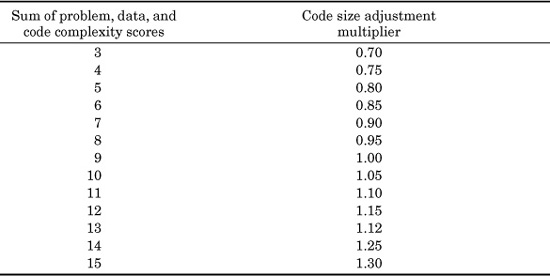
A great deal more research is needed on all forms of software complexity, and particularly on complexity associated with algorithms, visualization, software requirements, specifications, test cases, and data complexity.

Software Sizing with Reusable Components

As the second edition is being drafted, an increasingly large number of software projects are being constructed using reusable components of various kinds. The topic of reuse is very large and includes many more artifacts than source code alone. For example, it is possible to reuse any or all of the following software artifacts:

Reusable architectures

Reusable requirements

Reusable use cases or stories

Reusable designs

Reusable class libraries

Reusable source code modules

Reusable source code components

Reusable cost estimates

Reusable project plans

Reusable data

Reusable user manuals

Reusable graphics

Reusable test plans

Reusable test cases

To facilitate subsequent reuse, every reusable object should have its measured size included as part of the basic information that accompanies the reused artifact. However, as of 2007 the majority of reusable objects and artifacts lack accurate size information.

Sizing methods for dealing with reusable artifacts are not yet perfected as this book is being written, but they are starting to evolve. The eventual solution will probably be to enumerate function point totals, object point totals, or totals in some other metric for all major reusable artifacts, so that when software projects are constructed from reusable components their overall size can be summed from the function point sizes of the individual components.

Thus, it might be possible in the future to estimate a project that consists of 7 reusable components, each of 100 function points in size, plus a separate portion that must be developed uniquely that is 300 function points in size. Thus, the overall project as delivered will be 1000 function points, but it will be constructed from 700 function points of reusable components and one unique component of 300 function points.

A basic difficulty of this approach is the fact that generic reusable components may have features that are not needed or used by a specific application. For example, suppose that for a reusable component of 100 function points, only half of these, or 50 function points, are actually going to be utilized in the application being estimated.

The current solution to this problem is to assign a size label to the overall reusable component, and then use percentages to deal with the portions being used. For example, in the case just cited the gross size of the component is 100 function points, and if 50 percent of these features are to be utilized, then the net size in the current application would be 50 function points.

However, the introduction of percentages is intellectually unsatisfying and lacks precision. As this book is being written, there are no other available methods for dealing with partial utilization of reusable artifacts. Of course, improvements in the development of reusable objects might also minimize the quantities of included material that is not actually utilized.

Since functional metrics reflect the user’s view of the features needed or desired, it is obvious that if 1000 users are going to utilize portions of the same artifact, their personal needs will vary widely.

Consider a basic application, such as a modern Windows-based word processor, whose total size in terms of all features is perhaps 5000 function points. Modern word processors are so feature-rich that it is doubtful if any single user utilizes more than a fraction of their available capacity. For example, in writing this book using Microsoft Word it is unlikely that the author utilized more than about 10 percent of the total feature set of this product, or perhaps 500 function points out of a possible 5000 function points.

However, on any given business day millions of people are using Microsoft Word simultaneously, so all of us together probably exercise every known feature of this product on a daily basis, even though no single user needs more than a small fraction of the total capabilities.

This simple example illustrates a key point when dealing with software reusability. It is important to keep separate records for what is delivered to clients, what is developed by the project team, and what is reused from component or class libraries.

In the past, the size of what got delivered and the size of what was developed were close to being the same, and reuse usually amounted to less than 15 percent by volume. As component reuse, patterns, frameworks, object-oriented class libraries, and other forms of reuse become common there will be a marked transformation in the ratios of reused material to custom development. It is not impossible to envision future software projects where close to 100 percent of the major artifacts are reused and custom development hovers below 1 percent.

Incidentally, the use of ratios and percentages to distinguish the proportion of reused material for any given artifact is now a feature of the sizing logic of several commercial software cost-estimating tools. Users can now specify the percentage of reuse for such key artifacts as specifications, source code, user manuals, test cases, and so forth. The estimating tools will suggest default values based on empirical data, but users are free to modify the default assumptions for each artifact.

Overview of the Basic Forms of Software Sizing Metrics

The first edition of this book included a tutorial section on counting function points using the general rules from IFPUG. However, counting rules from IFPUG and other metrics groups tend to change annually. Also, many other function point variants exist and it is not possible to discuss the counting rules for all of these in less than about 500 pages.

For this second edition, a different approach is being used. Instead of a primer on IFPUG function point analysis, there are short discussions and pointers to sources of information about both IFPUG function points and other common sizing metrics. For those who actually wish to learn to count function points or the other metrics, taking a formal course followed by a certification examination is the best path. Tutorial books are also a good option. Because of rapid changes in counting rules and measurement technology, it is also useful to search the web for recent information.

It should be noted that actually counting functional metrics is not a trivial task. Usually, several days of training, numerous case studies, and guidance from a certified expert are needed to do this job well. Once a candidate has learned to count function points, passing a certification examination is the next step before actually attempting to count function points for clients or for situations where accuracy is needed. Counting function points is not a task for partly trained amateurs.

A controlled study found that certified function point counters who had passed the IFPUG exam had only about a 3 percent variation when counting the trial applications used for the study. Uncertified counters, on the other hand, can vary by more than 30 percent when counting the same application. Thus, certification is an important step in dealing with function point metrics with acceptable accuracy.

Following are short discussions of the more common metrics used for sizing circa 2007:

3D Function Points This variant was developed inside the Boeing corporation and published circa 1995. The 3D approach was intended for counting function points in a real-time environment. The 3D method produces larger counts for real-time software than standard IFPUG function points. Current usage circa 2007 is not known.

Backfiring from Physical LOC Backfiring is a method of converting the size of an application from source code volumes into an approximate number of function points. It is used primarily for legacy applications where code exists but no supporting specifications, so that conventional function point counting is impossible. Backfiring is as old as the function point metric itself. Allan Albrecht and his colleagues in IBM measured both source code volumes and function points while function point metrics were being developed and calibrated in the early 1970s. The starting point for backfiring can either be physical lines or logical statements. The Software Engineering Institute (SEI) has endorsed counts of physical lines of code as a metric for software projects. However, depending upon the programming language, there can be ranges of more than 3 to 1 between counts of physical lines of code and counts of logical statements. Backfiring from physical lines of code may sometimes come close actual counts of function points, but this form of backfiring can be off by more than 50 percent.

Backfiring from Logical Statements Mathematical conversion from source code volumes to function point metrics can start using counts of physical lines of code or counts of logical statements. Because some languages (such as Quick Basic) allow multiple statements to be placed on a single physical line, there are often major differences between counts of physical lines of code and counts of logical statements. In other languages (such as COBOL), a single logical statement can span several physical lines, such as might be found in case statements or “if . . . then” statements. Because of the random and uncertain nature of physical lines, backfiring from counts of logical statements is more consistent and often yields results that are closer to actual counts of function points. Unfortunately, it is harder to get accurate counts of logical statements. When used for backfiring purposes, conversion from logical statements often matches actual function point counts within about 20 percent. The main source of information on backfiring from logical statements is a large catalog of programming languages published by Software Productivity Research LLC (SPR). As of 2007, this catalog contains more than 600 languages and dialects. This catalog includes information on the number of logical source code statements for every known programming language. It also contains information on the ranges, since programmers tend to code in different styles. As might be expected, the observed range is directly proportional to the numbers of programmers who use a particular language. Common languages such as C and Java have very large ranges.

Complexity Metrics Complexity is an important topic that can affect the sizes of applications, their defect rates, their schedules, and their costs. Unfortunately, the software engineering community uses only fairly primitive methods for dealing with complexity. For sizing purposes, a subjective evaluation of complexity is part of the calculations for counting function point metrics. For evaluating software quality and defect levels, Tom McCabe’s cyclomatic and essential complexity metrics have long been used. The actual impact of various kinds of complexity on software size, costs, and error rates remains ambiguous circa 2007.

COSMIC Function Points Cosmic function points are one of the newer and more important variants to IFPUG function points. The word “COSMIC” stands for “Common Software Measurement Consortium,” which is an organization centered in Europe and the United Kingdom. The COSMIC function point method evolved from Dr. Alain Abran’s older “full function point” method coupled with some aspect of Charles Symon’s Mark II function point method. Members of the COSMIC group come mainly from Europe and the United Kingdom, although Canada, Japan, and Australia also have members. There are few if any members of the COSMIC organization from the United States. As with most function point variants, COSMIC function points produce larger totals for real-time software than do IFPUG function points. The COSMIC organization offers training and certification examinations. However, the COSMIC organization has not dealt with backfiring in a formal way, nor have they published conversion rules between IFPUG function points and COSMIC function points. The COSMIC approach is one of four methods certified by the International Standards Association.

Engineering Function Points This function point variant was published circa 1994 by Donald Ulmholtz and Arthur Leitgab. This metric starts with the usual IFPUG method but adds a new data element—algorithms. Therefore, engineering function points actually overlap the older feature point metric from 1986 that also added algorithms to the function point rules. There are few recent citations about engineering function points. Usage as of 2007 is unknown.

Feature Points The feature point metric was developed by the author circa 1986, in collaboration with Allan Albrecht, the inventor of function points. (Albrecht worked for Software Productivity Research for several years after retiring from IBM.) Feature points differed from IFPUG function points in several respects. A new parameter, “algorithms,” was introduced. The weight assigned to the “logical file” parameter was reduced. The method was developed to solve a psychological problem rather than an actual measurement problem. There was a misapprehension that function point measurements only applied to information systems. By using the name “feature points” and by introducing the algorithm parameter, a metric was introduced that appealed to the telecommunications and real-time domain. For more than 90 percent of all applications function points and feature points generated the same totals. Only for a few applications with a great many algorithms would feature points yield higher totals. Feature points were one of the few function point variants to offer conversion rules to standard IFPUG counts. After standard IFPUG function points began to be used for real-time and telecommunications software, there was no need for feature points. The primary citation and examples of feature points were in the author’s book Applied Software Measurement (McGraw-Hill publisher, 1996). Usage as of 2007 is unknown.

Full Function Points This metric was developed by Dr. Alain Abran of the University of Quebec. As with many function point variations, full function points yield higher counts for real-time software than standard IFPUG function points. Full function points had some usage in Canada, the United Kingdom, and Europe. The method had few if any users in the United States. The full function point metric was one of the precursors to the new COSMIC function point. The full function point method evolved over several years and had several different sets of counting rules. Conversion from full function points to IFPUG function points is not precise, but it has been observed that full function points create larger totals than IFPUG for real-time software by perhaps 15 percent. Full function points were publicized circa 1998. Now that the COSMIC approach has been released, usage of full function points circa 2007 is unknown.

IFPUG Function Points IFPUG stands for “International Function Point Users Group.” This is the oldest and largest software metrics association, with about 3000 members in perhaps 25 countries. IFPUG is a non-profit organization. Their web site is www.IFPUG.org. As background, function points were invented by Allan Albrecht and his IBM colleagues circa 1975. IBM was the keeper of function point counting rules from 1975 until 1986 when IFPUG was formed in Toronto, Canada. IFPUG moved to the United States in 1998. IFPUG publishes and updates the counting rules for function points (the current version is 4.1) and also runs training courses and certification exams. As of 2007, about 1500 people have passed the IFPUG certification exam. IFPUG function points consist of the totals of five external attributes of software: inputs, outputs, inquiries, logical files, and interfaces. Totals of these attributes are summed, and then adjusted for complexity. This sounds quite simple, but the actual counting rules are more than 100 pages long. It usually takes from two to three days of training before the certification exam can be successfully passed. As of 2007, IFPUG function points are in use for information systems, embedded software, real-time software, weapons systems, expert systems, and essentially all other forms of software. In side-by-side trials with some of the other function point variants, IFPUG tends to create somewhat lower totals than the other variants for real-time software. The IFPUG approach is one of four methods certified by the International Standards Organization.

ISO Standard 19761 for Functional Sizing The International Organization of Standards (ISO) has defined an overall standard for sizing software. This is ISO 19761, which was published in 2003. Currently, four function point methods have received ISO certification: COSMIC function points, IFPUG function points, Mark II function points, and NESMA function points. As this book is written, none of the object-oriented metrics such as object points, web object points, and use case points have been certified by ISO, nor have any of the lines-of-code-metrics. Backfiring has not been certified either. It should be noted that ISO certification does not guarantee accuracy of counts, nor consistency among unlike counting methods. However, ISO certification does indicate that a specific metric has followed a reasonable set of rules and is theoretically capable of being used to create fairly accurate size data.

Mark II Function Points The Mark II function point method is the oldest variant to standard IFPUG function points. The Mark II approach was first announced in London by Charles Symons in 1983. The Mark II approach was also documented in Symon’s book, Software Sizing and Estimating Mk II FPA (function point analysis) (John Wiley & Sons publisher, 1991). As with the other function point variants, the Mark II approach tends to produce higher totals than IFPUG function points for real-time and embedded software. Usage of the Mark II approach was most widespread in the United Kingdom, but there was also usage in other countries with historical ties to the U.K. such as Hong Kong, Ireland, and Australia. The Mark II method for evaluating complexity does contain some interesting extensions to the IFPUG approach. Some of these methods have migrated into the newer COSMIC function point approach. The Mark II approach is one of four methods certified by the International Standards Organization.

NESMA Function Points The acronym “NESMA” stands for the Netherlands Software Metrics Association. NESMA originated under a different name: Netherlands Function Point Users Group, or NEFPUG, in 1989. They changed their name circa 1995. The NESMA organization has about 120 member companies, almost 1000 individual members, and is a major European source for metrics information and function point certification. NESMA produces a function point standards manual that is based on IFPUG 4.1, but has some extensions and differences. As a result, the NESMA method for counting function points and the IFPUG method come fairly close to producing the same totals, but NESMA typically generates large totals for real-time software. The NESMA method is one of four approaches certified by the International Standards Organization.

Object Points There are several metrics that use the name “object points.” One of these was defined by D.R. Banker in 1994; there are also object points supported by Dr. Barry Boehm’s COCOMO II cost-estimating tool. Another method termed “web object points” was defined by the well-known software consultant, Donald Riefer, in 2002. Banker’s version of object points uses screens and reports to generate a kind of function point. This method is not actually derived from the object-oriented programming method. The second method, by Reifer, includes parameters based on multimedia files, scripts, links, hypertext, and other attributes of modern web-based applications. The Reifer approach adds these new parameters to standard IFPUG function points. As might be expected from the new parameters, it will produce larger counts than IFPUG function points for web-based applications. The Reifer approach also includes and supports back-firing, which is a rare feature among the function point variants. In spite of using the term “object points,” neither the Banker nor Reifer methods are actually derived from the canons of object-oriented programming. Usage of object points as of 2007 is unknown. However, the Reifer method was intended to operate in a COCOMO II environment, which is a widely used software cost-estimating tool. Therefore, the Reifer variant may have several hundred users.

SPR Function Points Software Productivity Research developed a minor function point variation in 1986 to simplify and speed up calculations. The SPR function point metric was developed in conjunction with Allan Albrecht, the inventor of function points. The main difference between SPR function points and standard function points was in simplifying the complexity adjustments. The SPR approach used three factors for complexity, each of which could be evaluated via a five-point scale: problem complexity, data complexity, and code complexity. The last factor, “code complexity,” was used to adjust the results when backfiring. It was not used for forward function point estimation. The SPR approach was designed to come as close as possible to the standard IFPUG method. However, the method in use at the time was IFPUG 3.0. The SPR approach was not updated to match IFPUG 4.0 or 4.1 because other methods supplanted it. The primary publication of the SPR approach was in the author’s book Applied Software Measurement, Second Edition (McGraw-Hill publisher, 1996). There were several hundred users of SPR function points in the 1990s, and some still use the method in 2007.

Story Points The term “story points” stems from a method used by the Agile development approach and by extreme programming (XP) in gathering requirements. User requirements are documented in the form of “user stories,” which are roughly analogous to use cases but more informal. Because user stories can range from very small to rather large, there was a need to have some form of metric for judging the relative size of a user story. The purpose of story points was to facilitate estimating the schedules and resources needed to develop the code for the story. Currently, story points are a subjective metric without certification or formal counting rules. In fact, one way of ascertaining the number of story points in a user story is called the “poker game” because team members open with their estimate of the number of story points, and other team members can check or raise. Because of the popularity of Agile and XP, there are hundreds or even thousands of users of story points circa 2007. However, the literature on story point sizes is sparse. Needless to say, story points are not certified by the International Standards Organization (ISO). From examining some stories and looking at story points, it can be hypothesized that a story point is more or less equivalent to two function points. An entire story is more or less equivalent to about 20 function points.

Use Case Points Use cases are one of the methods incorporated into the unified modeling language (UML), although they can be used separately if desired. Because of the widespread deployment of UML for object-oriented (OO) software, use cases have become quite popular since about 2000. A use case describes what happens to a software system when an actor (typically a user) sends a message or causes a software system to take some action. Use case points start with some of the basic factors of IFPUG function points, but add new parameters such as “actor weights.” Use case points also include some rather subjective topics such as “lead analyst capability” and “motivation.” Since both use case points and IFPUG function points can be used for object-oriented software, some side-by-side results are available. As might be expected from the additional parameters added, use case points typically generate larger totals than IFPUG function points by about 25 percent. One critical problem limits the utility of use case points. Use case points have no relevance for software projects where use cases are not being utilized. Thus, for dealing with economic questions such as the comparative productivity of OO projects versus older procedural projects that don’t capture requirements with use cases, the use case metric will not work at all. Because of the popularity of UML and use cases, the use case metric probably has several hundred users circa 2007. However, the use case metric is not one of those certified by the International Standards Organization. There are currently no certification exams for measuring the proficiency of metrics specialists who want to count with use cases. The approach is growing in numbers, but would benefit from more training courses, more text books, and either creating a user association or joining forces with an existing user group such as IFPUG, NESMA, or one of the others. Since use case metrics are irrelevant for older projects that don’t deploy use cases, the lack of conversion rules from use case metrics to other metrics is a major deficiency.

There are many complicated metrics used in daily life that we have learned to utilize and often take for granted, although few of us actually know how these metrics are counted or derived. For example, in the course of a normal day we may use the metrics of horsepower, octane ratings, and perhaps British thermal units (BTUs). We might discuss caloric content or cholesterol levels in various kinds of food. We may also discuss wind-chill factors. For day-to-day purposes, it is only sufficient that we know how to use these metrics and understand their significance. Very few people actually need to know how to calculate octane ratings or horsepower, so long as we feel fairly confident that published data is calculated honestly.

In the same vein, very few people need to understand how to count function points, but every software project manager and technical staff member should understand how to use them and should know ranges of productivity and quality results.

For example, every project manager should understand the following generic ranges of software productivity levels:

Projects of less than 5 function points per staff month (more than 26 work hours per function point) indicate performance that is below U.S. averages for all software projects.

Projects between 5 and 10 function points per staff month (13 to 26 work hours per function point) approximate the normal range for U.S. software projects.

Projects between 10 and 20 function points per staff month (7 to 13 work hours per function point) are higher than U.S. averages for software projects. Many object-oriented OO projects are in this range.

Projects above 20 function points per staff month (7 work hours per function point) are significantly better than U.S. averages for software projects. Many Agile projects are in this range, in part because many Agile projects are quite small.

Of course, this kind of generic information needs to be calibrated for the specific class of software being considered, and also for the size of specific applications. Small projects of less than 100 function points in size often top 20 function points per staff month, but for larger projects above 1000 function points in size such results are extremely rare.

Function point metrics are difficult to calculate but easy to understand. The basic range of performance using function point metrics should be known by all software practitioners even if they only know such generalities as the following:

A delivered defect rate of more than 1.50 bugs per function point is very bad.

A delivered defect rate of less than 0.75 bugs per function point is normal.

A delivered defect rate of less than 0.10 bugs per function point is very good.

Understanding productivity and quality data expressed in terms of function points should be part of the training of every software manager. Knowing how to count function points is a skill that is needed only by a comparatively few specialists.

In summary, the main strengths of function point metrics are the following:

Function points stay constant regardless of the programming languages used.

Function points are a good choice for full-life-cycle analysis.

Function points are a good choice for software reuse analysis.

Function points are a good choice for object-oriented economic studies.

Function points are supported by many software cost-estimating tools.

Function points can be mathematically converted into logical code statements for many languages.

The main weaknesses of function point metrics are the following:

Accurate counting requires certified function point specialists.

Function point counting can be time-consuming and expensive.

Function point counting automation is of unknown accuracy.

Function point counts are erratic for projects below 15 function points in size.

Function point variations have no accurate conversion rules to IFPUG function points.

Many function point variations have no backfiring conversion rules.

Although the technical strengths of function points are greater than their weaknesses, the politics and disputes among the function point splinter groups is distressing. The multiplicity of function point variants is confusing to non-specialists and somewhat embarrassing to the function point community itself.

On the other hand, the problems of using lines-of-code-metrics for sizing and estimating are even greater than those of functional metrics. The most effective strategy would probably be to concentrate on developing one or more standard functional metrics with rigorous conversion logic between the standard and older alternatives.

Source Code Sizing

Source code sizing is the oldest sizing method for software and has been part of the feature sets of software cost-estimating tools since the 1970s. In general, for such common programming languages as COBOL or C, automated software cost-estimating tools can now do a very capable job of source code size prediction as early as the requirements phase, and often even before that, by using some of the approximation methods discussed earlier.

However, sizing for modern visual programming languages has added some complexity and some ambiguity to the source code sizing domain. For such languages as Visual Basic, Realizer, Forte, PowerBuilder, and many others, some of the “programming” does not utilize source code statements at all.

Sizing source code when the language utilizes button controls, pull-down menus, or icons in order to create functionality is a difficult task that taxes software cost-estimating tools. But the usage of such controls for programming development is a fast-growing trend that will eventually dominate the software language world. It is also a trend that basically negates the use of source code metrics for some of the languages in question, although function points work perfectly well.

When the software industry began in the early 1950s, the first metric developed for quantifying the output of a software project was the metric termed lines of code (LOC). Almost at once some ambiguity occurred, because a line of code could be defined as either of the following:

A physical line of code

A logical statement

Physical lines of code are simply sets of coded instructions terminated by pressing the ENTER key of a computer keyboard. For some languages physical lines of code and logical statements are almost identical, but for other languages there can be major differences in apparent size based on whether physical lines or logical statements are used.

Table 9.7 illustrates some of the possible code counting ambiguity for a simple COBOL application, using both logical statements and physical lines.

TABLE 9.7 Sample COBOL Application Showing Sizes of Code Divisions Using Logical Statements and Physical Lines of Code

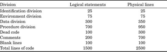
As can be seen from this simple example, the concept of what actually comprises a line of code is surprisingly ambiguous. The size range can run from a low of 700 LOC if you select only logical statements in the procedure division to a high of 2500 LOC if you select a count of total physical lines. Almost any intervening size is possible, and most variations are in use for productivity studies, research papers, journal articles, books, and so forth.

Bear in mind that Table 9.7 is a simple example using only one programming language for a new application. The SPR catalog of programming languages contains more than 600 programming languages, and more are being added on a daily basis. Furthermore, a significant number of software applications utilize two or more programming languages at the same time. For example, such combinations as COBOL and SQL, Ada and Jovial, and Java and HTML are very common. SPR has observed one system that actually contains 12 different programming languages.

There are other complicating factors, too, such as the use of macro instructions and the inclusion of copybooks, inheritance, class libraries, and other forms of reusable code. There is also ambiguity when dealing with enhancements and maintenance, such as whether to count the base code when enhancing existing applications.

Obviously, with so many variations in how lines of code might be counted, it would be useful to have a standard for defining what should be included and excluded. Here we encounter another problem. There is no true international standard for defining code counting rules. Instead, there are a number of published local standards which, unfortunately, are in conflict with one another.

Citing just two of the more widely used local standards, the SPR code-counting rules published in 1991 are based on logical statements while the SEI code-counting standards are based on physical lines of code. Both of these conflicting standards are widely used and widely cited, but they differ in many key assumptions.

As an experiment, the author carried out an informal survey of code-counting practices in such software journals as American Programmer, Byte, Application Development Trends, Communications of the ACM, IBM Systems Journal, IEEE Computer, IEEE Software, Software Development, and Software Magazine.

About a third of the published articles using LOC data used physical lines, and another third used logical statements, while the remaining third did not define which method was used and, hence, were ambiguous in results by several hundred percent. While there may be justifications for selecting physical lines or logical statements for a particular research study, there is no justification at all for publishing data without stating which method was utilized!

To summarize, the main strengths of physical LOC are as follows:

The physical LOC-metrics is easy to count.

The physical LOC-metrics has been extensively automated for counting.

The physical LOC-metrics is used in a number of software estimating tools.

The main weaknesses of physical LOC are as follows:

The physical LOC-metrics may include substantial dead code.

The physical LOC-metrics may include blanks and comments.

The physical LOC-metrics is ambiguous for mixed-language projects.

The physical LOC-metrics is ambiguous for software reuse.

The physical LOC-metrics is a poor choice for full-life-cycle studies.

The physical LOC-metrics does not work for some visual languages.

The physical LOC-metrics is erratic for direct conversion to function points.

The physical LOC-metrics is erratic for direct conversion to logical statements.

The main strengths of logical statements are as follows:

Logical statements exclude dead code, blanks, and comments.

Logical statements can be mathematically converted into function point metrics.

Logical statements are used in a number of software estimating tools.

The main weaknesses of logical statements are as follows:

Logical statements can be difficult to count.

Logical statements are not extensively automated.

Logical statements are a poor choice for full-life-cycle studies.

Logical statements are ambiguous for some visual languages.

Logical statements may be ambiguous for software reuse.

Logical statements may be erratic for direct conversion to the physical LOC-metrics.

Although not as exotic as the modern visual programming languages, a number of important business applications have been built with spreadsheets such as Excel and Lotus. The mechanics of entering a spreadsheet formula are more or less equivalent to using a statement in a programming language. The spreadsheet macro languages actually are programming languages, if not very elegant ones. However, using the built-in spreadsheet facilities for creating graphs from numeric tables is not really programming as it is traditionally defined.

Even more troublesome in the context of sizing are some of the add-on features associated with spreadsheets, such as templates, backsolving features, functions for statistical operations, for “what you see is what you get” printing, and a host of others.

For example, Case Study A earlier in this book illustrated a cost estimate for a small personal travel expense program that was to be created in Visual Basic. Several commercial spreadsheets already have travel expense templates available, so that if the application were intended for a spreadsheet rather than for Visual Basic, little or no programming would even be needed.

Indeed, even in the context of Visual Basic, travel expense controls are available from commercial vendors, which would cut down on the amount of procedural code that might have to be created.

Of course, reused software code in any fashion adds complexity to the task of software sizing also. Spontaneous reuse by programmers from their own private libraries of algorithms and routines has been part of programming since the industry began.

More extensive, formal reuse of software artifacts from certified libraries or commercial sources is not as common as private reuse, but is rapidly becoming a trend of significant dimensions.

As mentioned previously, there are more than 500 variations and dialects of commercial programming languages in existence, and perhaps another 200 or so proprietary “private” languages have been developed by corporations for their own use.

Also, many software applications utilize multiple languages concurrently. About one-third of U.S. software projects contain at least two programming languages, such as COBOL and SQL. Perhaps 10 percent of U.S. software applications contain three or more languages, and a few may contain as many as a dozen languages simultaneously.

The technology of source code size prediction for traditional procedural programming languages has been eased substantially by the advent of function point metrics. Because function points are normally calculated or derived during requirements definition, and because source code volumes can be predicted once function point totals are known, it is now possible to create reasonably accurate source code size estimates much earlier in the development cycle than ever before.

However, even with the help of function points source code sizing has some problems remaining, as shown in Table 9.8.

TABLE 9.8 Software Sizing Problems Circa 2007

The same application can vary by as much as 500 percent in apparent size depending upon which code counting method is utilized. Consider the following example in the BASIC programming language:

   BASEPAY = 0: BASEPAY5HOURS*PAYRATE: PRINT BASEPAY

This example is obviously one physical line of code. However, this example contains three separate logical statements. The first statement sets a field called BASEPAY to zero value. The second statement performs a calculation and puts the result in the field called BASE-PAY. The third statement prints out the results of the calculation.

It is clearly important to know whether physical lines or logical statements are implied when using the phrases lines of code (LOC), 1000 lines of code (KLOC), and 1000 source lines of code (KSLOC). (There is no difference numerically between KLOC and KSLOC.)

As a general rule, sizing source code volumes lends itself to rule-based parsing engines that can examine large volumes of source code quickly. While such engines are commercially available for such common languages as COBOL and C, the organizations that utilize proprietary or obscure languages often build their own counting tools.

Unfortunately, there is little or no consistency in the rules themselves, and almost every conceivable variation can be and has been utilized. The wide variations in methods for enumerating source code volumes cast severe doubts on the validity of large-scale statistical studies based on LOC-metrics.

If one-third of the journal articles use physical lines of code, one-third use logical statements, and one-third don’t state which method is used, then it is obvious that the overall data based on LOC-metrics needs some serious scrubbing before any valid conclusions might be derived from it.

Once the primary size of a software project is determined using function points, source code statements, or both, then a host of other software artifacts can be sized in turn. Let us now consider some of the sizing ranges for such derivative software artifacts as paper documents, test cases, and bugs or defects.

Sizing Object-Oriented Software Projects

The object-oriented (OO) paradigm has been expanding rapidly in terms of numbers of projects developed. The OO paradigm presents some interesting challenges to software cost-estimating and sizing tool vendors, since OO development methods are not perfectly congruent with the way software is developed outside of the OO paradigm.

The OO community has been attempting to quantify the productivity and quality levels of OO projects. To this end, several OO metrics have been developed including use case points and several flavors of object points. Because of the special needs of the OO paradigm the traditional LOC-metric was not a suitable choice.

Although function point metrics can actually demonstrate the productivity advantages of the OO paradigm and have been used for OO economic analysis knowledge of functional metrics remains comparatively sparse among the OO community even in 2007.

Curiously, the function point community is very knowledgeable about the OO paradigm, but the reverse is not true. For example, Software Engineering Management Research Lab at the University of Montreal has produced an interesting report that mapped the older Jacobsen OO design method into equivalent function point analysis and generated function point sizes from Jacobsen’s design approach.

A fairly extensive form of software research has started among OO metrics practitioners to develop a new and unique kind of sizing and estimating for OO projects, based on a specialized suite of metrics that are derived from the OO paradigm itself. For example, research at the University of Pittsburgh has attempted to build a complete OO metrics suite.

Similar research is ongoing in Europe, and a suite of OO metrics termed MOOD has been developed in Portugal. There are also object point metrics, which attempt to build a special kind of function point keyed to the OO paradigm. Use case points and web object points are also used by OO practitioners.

In the United States the work of Chidamber and Kemerer is perhaps the best known. Some of the OO metrics suggested by Chidamber, Darcy, and Kemerer include the following:

Weighted Methods per Class (WMC) This metric is a count of the number of methods in a given class. The weight portion of this metric is still under examination and is being actively researched.

Depth of Inheritance Tree (DIT) This is the maximum depth of a given class in the class hierarchy.

Number of Children (NOC) This is the number of immediate subclasses of a given class.

Response for a Class (RFC) This is the number of methods that can execute in response to a message sent to an object within this class, using up to one level of nesting.

Lack of Cohesion of Methods (LCOM) This metric is a count of the number of disjoint method pairs minus the number of similar method pairs. The disjoint methods have no common instance variables, while the similar methods have at least one common instance variable.

As this edition is being written, the OO metrics are still somewhat experimental and unstandardized. None of the OO metrics, for example, have been certified by the International Standards Organization nor do they follow the guidelines of the ISO standard for functional sizing.

In the past, both LOC and function point metrics have splintered into a number of competing and semi-incompatible metric variants. There is some reason to believe that the OO metrics community will also splinter into competing variants, possibly following national boundaries. The main strengths of OO metrics are as follows:

The OO metrics are psychologically attractive within the OO community.

The OO metrics appear to be able to distinguish simple from complex OO projects.

The OO metrics can measure productivity and cost within the OO paradigm.

The OO metrics can measure quality within the OO paradigm.

The main weaknesses of OO metrics are as follows:

The OO metrics do not support studies outside of the OO paradigm.

The OO metrics do not deal with full-life-cycle issues.

The OO metrics have not yet been applied to testing.

The OO metrics have not yet been applied to maintenance.

The OO metrics have no conversion rules to LOC-metrics.

The OO metrics have no conversion rules to other function point metrics.

The OO metrics lack automation.

The OO metrics lack certification.

The OO metrics do not adhere to the ISO standards for functional sizing.

The OO metrics are not supported by software estimating tools.

Because of the rapid growth of the OO paradigm, the need for sizing and estimating metrics within the OO community is fairly urgent. Upon examination, use case points, web object points, object points, metrics for object-oriented software engineering (MOOSE) and metrics for object-oriented design (MOOD) metrics suites have some interesting technical features. Unfortunately, the OO metrics researchers have lagged in creating conversion rules between OO metrics and older metrics. This means that none of the OO metrics are able to deal with side-by-side comparisons between OO projects and procedural projects. This limits the usefulness of OO metrics to operating purely within an OO context, and bars them from dealing with larger economic and quality issues where statistical analysis of many kinds of projects are part of the analysis.

Sizing Text-Based Paper Documents

Software is a very paper-intensive occupation and tends to put out massive quantities of paper materials. In fact, for large military software projects the creation and production of paper documents is actually the major cost element; it is more expensive than the source code itself and is even more expensive than testing and defect removal.

For civilian projects, paperwork is not quite as massive as for military projects, but it can still run up to many thousands of pages for large systems above 5000 function points in size. Indeed, it is the high cost of software paperwork that was the impetus in creating some of the Agile development approaches. Extensive paperwork in the form of large and possibly ambiguous requirements documents and formal specifications are viewed by the Agile community as barriers to effective development rather than necessary precursors to coding.

Some of the major categories of paper documents produced for software projects include but are not limited to the following ten categories:

Planning documents

Requirements

Specifications

User manuals

Training materials

Marketing materials

Defect reports

Financial documents

Memos and correspondence

Contracts and legal documents

Sizing paper deliverables is a major feature of software cost-estimating tools and is a major topic for real-life software projects.

Sizing paper documents is especially important in a military software context, because military standards trigger the production of more paper than any other triggering factor in human history. The classic DoD 2167 standard has probably caused the creation of more pages of paper than any other technical standard in the world. Even the newer DoD 498 standard tends to generate significant volumes of paper materials.

Interestingly, the newer ISO 9000–9004 quality standards are giving DoD 2167 quite a good race for the record for most paperwork produced for a software project.

Curiously, many of these required military software documents were not really needed for technical reasons, but are there because the Department of Defense has a long-standing distrust of its many vendors. This distrust has manifested itself in the extensive oversight requirements and the massive planning, reporting, and specification sets mandated by such military standards as DoD 2167 or DoD 498.

The same sense of distrust is also found in the ISO 9000–9004 standard set and in ISO 9001 in particular. For an activity as common as performing software inspections and testing software applications, it should not be necessary to create huge custom test plans for every application. What the ISO standards and the DoD standards might have included, but did not, are the skeleton frameworks of review, inspection, and test plans with an assertion that special test-plan documentation would be needed only if the standard plans were not followed.

For commercial software projects, the internal specifications are not as bulky as for military or for systems software, but the external user manuals and the tutorial information are both large and sometimes even elegant, in terms of being produced by professional writers and professional graphics artists.

Among our civilian client organizations paperwork production ranks as the second most expensive kind of work on large systems, and is outranked only by the costs of defect removal, such as testing.

(Coding, by the way, is often as far down the list of software elements as fourth place. Coding expenses on large systems often lag behind paperwork costs, defect-removal costs, and meetings and communications costs.)

A minor but tricky issue for sizing software paperwork volumes is that of adjusting the size estimate to match the kind of paper stock being used.

For example, a normal page of U.S. office paper in the 8.5-by 11-inch format holds about 500 English words, although the inclusion of graphics and illustrations lowers the effective capacity to around 400 words. However, the common European A4 page size holds about 600 English words, while legal paper holds about 675 English words.

By contrast, the smaller page size used by the U.S. civilian government agencies only holds about 425 words. Thus, in order to predict the number of pages in specifications and user manuals, it is obvious that the form factor must be known.

Of course, the full capacity of a printed page for holding text is seldom utilized, because space is often devoted to the inclusion of graphical materials, which will also be discussed as an interesting sizing problem.

Table 9.9 illustrates how function point metrics are now utilized for producing size estimates of various kinds of paper documents. The table assumes normal 8.5-by 11-inch U.S. paper and IFPUG Version 4.1 function point rules.

Table 9.9 and the following illustrate a major benefit of function point metrics in the context of software sizing and cost estimating. Because the function point total for an application stays constant regardless of which programming language or languages are utilized, function points provide a very stable platform for sizing and estimating non-code artifacts, such as paper documents.

In fact, some of the LOC-based estimating tools don’t deal with paper deliverables or non-coding work at all.

Table 9.9 shows selected size examples, drawn from systems, MIS, military, and commercial software domains. In this context, systems software is that which controls physical devices, such as computers or telecommunication systems.

TABLE 9.9 Number of Pages Created per Function Point for Software Projects

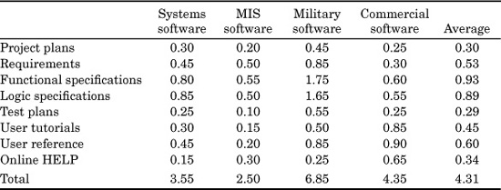
MIS stands for management information systems software and refers to the normal business software used by companies for internal operations.

Military software constitutes all projects that are constrained to follow various military standards.

Commercial software refers to ordinary packaged software, such as word processors, spreadsheets, and the like.

This kind of sizing for software documentation is now a standard feature of several commercial software cost-estimating tools. Indeed, as many as 50 discrete document types may be found on very large software projects. Table 9.10 is a summary list of the various kinds of paper documents associated with software projects.

TABLE 9.10 Examples of Paper Documents Associated with Software Projects

Although few projects will produce all of the kinds of information listed in Table 9.10, many software projects will create at least 20 discrete kinds of paper and online documentation. Given the fact that between 20 percent and more than 50 percent of software project budgets can go to the production of paper and online documents, it is obvious that paperwork sizing and cost estimating are important features of modern software cost-estimating tools.

Several commercial software estimating tools can even predict the number of English words in the document set, as well as the numbers of diagrams that are likely to be present, and can change the page-count estimates based on type size or paper size.

Since the actual sizing algorithms for many kinds of paper documents are proprietary, Table 9.11 is merely derived by assuming a ratio of 500 words per page, taken from Table 9.11.

As can easily be seen from Tables 9.10 and 9.11, software is a very paper-intensive occupation, and accurate software cost estimating cannot ignore the production of paper documents and achieve acceptable accuracy. Far too great a percentage of overall software costs are tied up in the creation, reviewing, and updating of paper documents for this cost factor to be ignored.

To illustrate the overall magnitude of software paperwork, the author has worked on several large systems in the 10,000–function point category where the total volume of pages in the full set of design and specification documents exceeded 60,000 pages.

TABLE 9.11 Number of English Words per Function Point for Software Projects

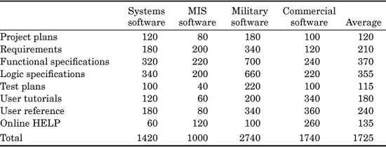
As a more extreme case, the sum of the paper documents for a proposed new operating system that IBM was considering would have totaled more than 1 million pages. The specifications would have been so large that reading them would exceed the lifetime reading speed of normal adults if they read steadily for eight hours every day for an entire career!

Should it have gone to completion, the full set of paper documents for the “Star Wars” strategic defense initiative, following normal military standards, would have exceeded 1 billion pages, and the sum of the English words would have exceeded 500 billion.

Although the document size information in this book is based on U.S. paper sizes and English words, software is an international discipline. Some software cost-estimating tools can deal with the same problems as they might be encountered in France, Germany, Japan, or other countries that both use different languages and have different conventions for paper sizes.

In addition, some kinds of software, such as commercial packages, need to be nationalized, or translated into multiple languages. For example, the author’s own KnowledgePlan cost-estimating tool is available in English, Japanese, and French versions. Large commercial software vendors, such as Computer Associates, IBM, and Microsoft, may have software materials translated into more than a dozen languages.

Another tricky but important aspect of dealing with software paperwork costs is producing estimates for multinational projects, where the primary specifications are in a single language, such as English, but the development team may comprise personnel from France, Japan, Russia, the Ukraine, and many other countries as well. Although the developers may be able to deal with English-language specifications, there may be a need for supplemental materials created in other languages.

Some cost-estimating tools can also estimate the added costs for translating tutorial materials, HELP screens, and even source code comments from one natural language to another.

Translation costs can be a rather complicated topic for languages that do not use the same kinds of symbols for representing information. For example, translating materials from English into Japanese or Chinese written forms is a great deal more costly than merely translating English into French or Spanish. Indeed, automated translation tools are available that can facilitate bidirectional translations between English and many European languages.

Another critical aspect of sizing software paperwork volumes is the fact that the volumes are not constant, but grow during the development cycle (and afterwards) in response to creeping user requirements.

Thus, software paperwork sizing algorithms and predictive methods must be closely linked to other estimating capabilities that can deal with creeping user requirements, deferrals of features, and other matters that cause changes in the overall size of the application.

It is obvious why visualization is such an important technology for software, and why software cost-estimating tools need to be very thorough in sizing and estimating paperwork for large software applications. Indeed, for almost all large systems in excess of 1000 function points in size, the total effort devoted to the construction of paper documents is actually greater than the effort devoted to coding. In the case of large military systems, the effort devoted to the creation of paper documents can be more than twice as costly as coding.

Sizing Graphics and Illustrations

Software specifications, software user manuals, software training materials, and sometimes online software tutorials often make extensive use of graphics and visual information. The kinds of graphical materials associated with software projects include but are not limited to the following categories:

Application design graphics

Planning and scheduling graphics

Charts derived from spreadsheets

Illustrations in user manuals

Graphical user interfaces (GUIs)

Photographs and clip art

Graphics sizing is a complicated undertaking because there are so many possibilities. In the modern world of web-based applications, graphics are the primary user interface. Indeed, some of the graphical elements are dynamic in the form of video or animation. For example, in just the software design category alone there are at least 50 major dialects of graphical software specification methods in existence, such as those listed in Table 9.12.

Not only are there many different dialects or flavors of graphics-based software specification methods, but many projects use combinations of these diverse approaches rather than a single pure approach. For example, it is very common to see a mixture of flowcharts, one or more of the object-oriented specification methods, and some kind of entity-relationship charts all in the specifications for a single project.

Even more difficult from the standpoint of software sizing and cost estimating, a significant number of companies have developed unique and proprietary variants of common design methods that only they utilize. For example, the ITT corporation used the structured analysis and design technique (SADT) in both its pure form, and also in the form of a customized ITT variation created for switching software projects.

TABLE 9.12 Forms of Graphical Software Design Representations

Table 9.13 illustrates the approximate volumes of graphic items per function point in various document types. A graphic item can be any of the following:

A flowchart page

An entity-relationship chart

A data-flow diagram

A control-flow diagram

A use case diagram

A UML diagram (in about 13 flavors)

A Gantt chart

A PERT chart

A Kiviat graph

A graph from a spreadsheet, such as Excel or Lotus

An illustration from a graphics package, such as PowerPoint

A photograph

Needless to say, Table 9.13 has a significant margin of error and should be used only to gain an understanding of the significant volumes of graphical materials that are likely to be produced for software projects.

The ability of modern software cost-estimating tools to deal with the size ranges of both text and graphics is one of the features that makes such tools useful.

Too often, manual estimates by software project managers tend to ignore or understate the non-coding portions of software projects, because the managers have comparatively little familiarity with the paper and graphics side of software.

TABLE 9.13 Number of Graphics Items per Function Point for Software Projects

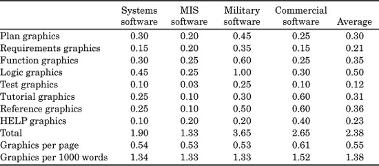
Sizing Bugs or Defects

As software projects grow from less than 1000 function points to more than 10,000 function points in size, the costs, effort, and schedules associated with defect-removal operations tend to become the largest and costliest component of the entire project.

Also, when software projects miss their schedules (as in the case of the Denver airport) it is almost always due to a quality problem that keeps the software from running well enough to go into full production.

Of all of the factors that need to be estimated carefully, the number of bugs or errors is the most critical. Two major aspects of bug or defect prediction are now features of several software cost-estimating tools:

Predicting the number of bugs by origin point and severity levels

Predicting the efficiency of various inspections and tests in removing bugs

Software defect prediction is another area where commercial software cost-estimating tools can outperform even experienced human managers. The reason is that software cost-estimating tools are operating from the basis of several thousand projects, while human managers may see fewer than 50 projects in their entire careers.

The function point metric has expanded the ability to create accurate quality estimates and defect predictions. Prior to the advent of function point metrics, much of the software quality literature and most of the defect-prediction algorithms dealt only with coding defects. Now that function points are widely used, the ability to measure and predict software defects has expanded to include five significant categories:

Requirements defects

Design and specification defects

Coding defects

User documentation defects

Bad fixes, or secondary defects

Three new kinds of software defect prediction capabilities are not yet found in commercial software cost-estimating tools, but research is nearing the stage where predictive algorithms can be developed:

Test-case defects

Data and database defects

Web content defects

All three of these new categories of software defects have cost and schedule implications. Research performed at IBM indicates that software test cases sometimes contain more defects or errors than the software the test cases have been created to test!

The whole topic of data quality is becoming increasingly important. Research into data quality has suffered from the fact that there is no known metric for normalizing database volumes or data defects. In other words, there is no data point metric that is the logical equivalent to the function point metric.

Now that web projects are exploding in numbers and business importance, errors in web content are increasing in both number and economic consequences.

The well-known aphorism that “you can’t manage what you can’t measure” has long been true for software quality. For about 50 years, less than 5 percent of U.S. companies had measurement programs for software quality. Similar proportions have been noted in the United Kingdom and in Europe. Therefore, attempts to improve software quality tended to resemble the classic probability example called the drunkard’s walk. Quality improvements would lurch erratically in different directions and not actually get very far from the origin point.

When exploring why software quality measurements have seldom been performed, a basic issue has always been that the results were not very useful. A deeper analysis of this problem shows that an important root cause of unsuccessful quality measurement can be traced to the use of the flawed LOC-metrics.

Quality measurements based on lines of code have tended to ignore quality problems that originate in requirements and design and are of no use at all in measuring defects in related documents, such as user manuals. LOC-metrics have no relevance for databases and web content either. When the problems and errors of non-code software deliverables were accumulated, it was discovered that more than half of all software errors or defects were essentially invisible using LOC-metrics.

Historically, software quality was measured in terms of defects per 1000 source code statements, or 1000 lines of code (KLOC).

Unfortunately, the KLOC metric contains a built-in paradox that causes it to give erroneous results when used with newer and more powerful programming languages, such as Ada, object-oriented languages, or program generators.

The main problem with the KLOC metric is that this metric conceals, rather than reveals, important quality data. For example, suppose a company has been measuring quality in terms of defects per KLOC. A project coded in FORTRAN might require 10,000 LOC, and might contain 200 bugs, for a total of 20 defects per KLOC.

Now, suppose the same project could be created using a more powerful language, such as C++, which would require only 2000 lines of code and contain only 40 bugs. Here, too, there are 20 defects per KLOC, but the total number of bugs is actually reduced by 80 percent.

In the preceding FORTRAN and C++ examples, both versions provide the same functions to end users, and so both contain the same number of function points. Assume both versions contain 100 function points.

When the newer defects per function point metric is used, the FORTRAN version contains 2.00 defects per function point, but the C++ version contains only 0.40 defects per function point. With the function point metric, the substantial quality gains associated with more powerful high-level languages can now be made clearly visible.

Another problem with LOC-metrics is the difficulty of measuring or exploring defects in non-code deliverables, such as requirements and specifications. Here, too, function point metrics have illuminated data that was previously invisible.

Based on a study published in the author’s book Applied Software Measurement (McGraw-Hill, 1996, the average number of software errors in the United States is about five per function point. Note that software defects are not found only in code, but originate in all of the major software deliverables, in approximately the quantities shown in Table 9.14.

These numbers represent the total numbers of defects that are found and measured from early software requirements definitions throughout the remainder of the life cycle of the software. The defects are discovered via requirement reviews, design reviews, code inspections, all forms of testing, and user problem reports.

Unmeasured and practically unmeasurable in 2007 are defects found in test cases, in databases, and in web content. From the author’s attempts to quantify these, some very preliminary numbers are now possible:

Test case errors approximate 2.0 defects per function point.

Database errors approximate 6.0 defects per function point.

Web content errors approximate 4.0 defects per function point.

TABLE 9.14 U.S. Averages in Defects per Function Point Circa 2007

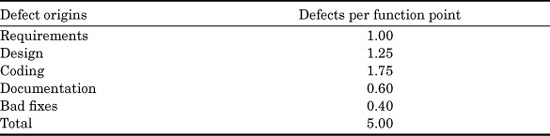
In other words, the volume of “invisible” defects that have not yet been measured because of a lack of suitable metrics is possibly more than twice as large as the volume of defects that are currently being measured.

U.S. averages using function points lend themselves to graphical representation. The graph in Figure 9.1 shows defect-potentials and defect-removal efficiency levels as the two axes. The graph also identifies three zones of some significance:

The central zone of average performance, where most companies can be found.

The zone of best-in-class performance, where top companies can be found.

The zone of professional malpractice, where companies that seem to know nothing at all about quality can be found.

It is very revealing to overlay a sample of an enterprise’s software projects on this graph. Note that the defects per FP axis refers to the total defect potential, which includes errors in the requirements, specifications, source code, user manuals, and bad fix categories.

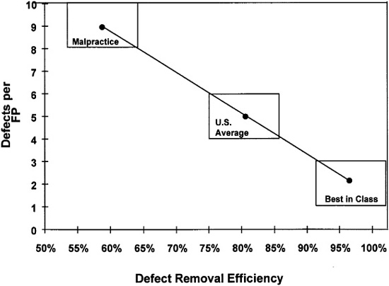
Figure 9.1 U.S. software quality performance ranges.

Complementing the function point metric are measurements of defect-removal efficiency, or the percentages of software defects removed prior to delivery of the software to clients.

The U.S. average for defect-removal efficiency, unfortunately, is currently only about 85 percent, although top-ranked projects in such leading companies as AT&T, IBM, Motorola, Raytheon, and Hewlett-Packard achieve defect-removal efficiency levels well in excess of 99 percent on their best projects and average close to 95 percent.

All software defects are not equally easy to remove. Requirements errors, design problems, and bad fixes tend to be the most difficult. Thus, on the day when software is actually put into production, the average quantity of latent errors or defects still present tends to be about 0.75 per function point, distributed as shown in Table 9.15, which also shows approximate ranges of defect-removal efficiency by origin point of software defects.

Note that at the time of delivery, defects originating in requirements and design tend to far outnumber coding defects. Data such as this can be used to improve the upstream defect-prevention and defect-removal processes of software development.

The best results in terms of defect removal are always achieved on projects that utilize formal pretest inspections of design, code, and other major deliverables, such as user manuals, and even test cases.

It is obvious that no single defect-removal operation is adequate by itself. This explains why best-in-class quality results can be achieved only from synergistic combinations of defect prevention, reviews or inspections, and various kinds of test activities.

The best software projects within the organizations that constitute roughly the upper 10 percent of the groups that SPR has assessed have achieved remarkably good quality levels. Following are software quality targets derived from best-in-class software projects and organizations:

Defect potentials of less than 2.5 defects per function point. (Sum of defects found in requirements, design, code, user documents, and bad fixes.)

TABLE 9.15 Defect-Removal Efficiency by Origin of Defect (Expressed in defects per function point)

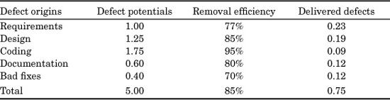
Cumulative defect-removal efficiency averages higher than 95 percent. (All defects found during development, compared to first year’s customer-reported defects.)

Average less than 0.025 user-reported defects per function point per year. (Measured against valid, unique defects.)

Achieve 90 percent excellent ratings from user-satisfaction surveys. (Measured on topics of product quality and service.)

Allow zero error-prone modules in released software. (Modules receiving more than 0.8 defects per function point per year.)

Improve software quality via defect prevention and defect removal at more than 40 percent per year. (Baseline is the current year’s volume of customer-reported defects.)

If your organization is approaching or achieving these results, then you are part of a world-class software production organization.

There are thousands of ways to fail when building software applications, and only a very few ways to succeed. It is an interesting phenomenon that the best-in-class companies in terms of quality all use essentially similar approaches in achieving their excellent results. The 12 attributes of the best-in-class quality organizations are listed in Table 9.16.

The similarity of approaches among such companies as AT&T, Bellcore, Hewlett-Packard, IBM, Microsoft, Motorola, Raytheon, and so forth is quite striking when side-by-side benchmark comparisons are performed.

The SEI maturity level concept is one of the most widely discussed topics in the software literature. SPR was commissioned by the U.S. Air Force to perform a study on the economic impact of various SEI capability maturity levels (CMM). Raw data was provided to SPR on levels 1, 2, and 3 by an Air Force software location.

TABLE 9.16 Common Attributes Noted in Best-in-Class Software Organizations

In terms of quality, the data available indicated that for maturity levels 1, 2, and 3 average quality tends to rise with CMM maturity level scores. However, this study had a limited number of samples. By contrast, the U.S. Navy has reported a counterexample, and has stated that at least some software produced by a level 3 organization was observed to be deficient.

There is clearly some overlap among the various SEI levels. Some of the software projects created by organizations at SEI level 2 are just as good in terms of quality as those created by SEI level 3. Indeed, there are even good-to excellent-quality projects created by some SEI level 1 organizations. Table 9.17 shows some suggested quality targets for the five plateaus of the SEI capability maturity model.

Above level 3 these targets are somewhat hypothetical, but from observations of organizations at various CMM levels the results would seem to be within the range of current technologies through level 4.

For level 5, the hardest part of the target would be dropping the potential defect level down to 1 per function point. Achieving a 99 percent cumulative defect-removal efficiency level is actually possible with current technologies for projects using formal inspections, testing specialists, and state-of-the-art testing tools.

As can be seen, the combination of function point metrics and defect-removal efficiency metrics are beginning to clarify quality topics that have long been ambiguous and intangible. Some of the examples shown here are now standard features of software cost-estimating tools.

It cannot be overemphasized that quality estimates and cost estimates are closely coupled, because the costs and schedule time required for defect-removal operations make up the largest component of software expense elements.

Software quality measurement and estimation should not be limited only to source code. Every major software deliverable should be subject to careful quality analysis, including but not limited to software requirements, specifications, planning documents, and user manuals. However, the LOC-metrics is not effective in dealing with non-code software deliverables.

TABLE 9.17 SEI CMM Software Quality Targets for Each Level (Expressed in defects per function point)

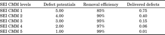
The combination of function point metrics coupled with direct measurement of defect-removal efficiency levels is making software quality results tangibly demonstrable. Now that software quality can be measured directly and predicted accurately, significant improvements are starting to occur.

Sizing Test Cases

The effort, costs, and schedule time devoted to testing software can, in some cases, exceed the effort, costs, and time devoted to coding the software. This situation means that test case sizing and testing estimation are critical features of software cost-estimating tools.

Fortunately, the function point metric has made a useful contribution to the ability to predict test case volumes. Recall the fundamental structure of function points:

Inputs

Outputs

Logical files

Inquiries

Interfaces

These factors are the very aspects of software that need to be tested and, hence, the function point metric is actually one of the best tools ever developed for predicting test case volumes, because derivation from function points is an excellent way of dealing with a problem that was previously quite difficult.

An emerging and very important topic in the context of test estimating is that of predicting the number of bugs or errors in test cases themselves. As many commercial software vendors have come to realize, the error density of software test cases may actually exceed the error density of the software being tested. As previously noted, the defect volume in test libraries approximates 2.0 defects per function point. This means that there may be more defects in test cases than in the code being tested!

Because function points can be derived during both the requirements and early design stages, this approach offers a method of predicting test case numbers fairly early. The method is still somewhat experimental, but the approach is leading to interesting results and its usage is expanding.

Table 9.18 shows preliminary data for 18 kinds of testing on the number of test cases that have been noted among SPR’s clients, using test cases per function point as the normalizing metric.

TABLE 9.18 Range of Test Cases per Function Point for 18 Forms of Software-Testing Projects in the United States

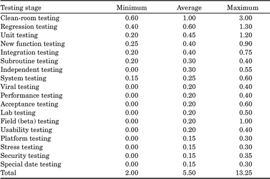
This table has a high margin of error, but as with any other set of preliminary data points, it is better to publish the results in the hope of future refinements and corrections than to wait until the data is truly complete.

It should be noted that no project in our knowledge base has utilized all 18 forms of testing concurrently. The maximum number of test stages that the author has observed has been 16.

Much more common is a series of about half a dozen discrete forms of testing, which would include the following:

Subroutine testing

Unit testing

New function testing

Regression testing

System testing

Acceptance or field testing

Another way of looking at test case sizing is in terms of the patterns of testing by industry, rather than simply examining all 18 kinds of testing (see Table 9.19).

As can be seen, the numbers of test cases produced will vary widely, but quite a bit of this variance can be reduced by utilizing the typical patterns found in the class and type of software application.

TABLE 9.19 Number of Test Cases Created per Function Point

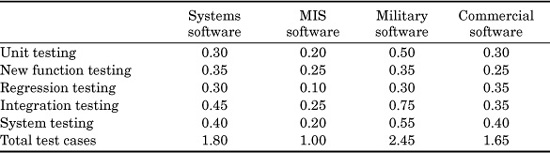
To a very significant degree, modern software cost-estimating tools operate as pattern-matching engines. Once the nature, scope, class, and type parameters are known to the software cost-estimating tool, it can begin to extract and utilize similar projects from its built-in knowledge base or from the portfolio of projects stored by users.

Of course, there is always a finite probability that any given project will deviate from the normal patterns of its class and type. This is why software cost-estimating tools allow users to override many predictions and make adjustments to the estimating assumptions.

Although functional metrics are not perfect, the advent of function points has expanded the number of software artifacts that can be sized, and has greatly simplified the tasks of sizing multiple deliverables.

The Event Horizon for Sizing Software Artifacts

We are now approaching the event horizon for software sizing technology. Beyond this horizon are a number of software artifacts where sizing is outside the scope of current software estimation capabilities.

Sizing Database Volumes

The technology for sizing database volumes is far less sophisticated than the technology for sizing other artifacts, such as documents, source code, test cases, and defects. The reason for this is because there are no current metrics for enumerating either the size of a database or for normalizing the number of errors that a database may contain.

Sizing Multimedia Artifacts

Modern software packages distributed and executed via CD-ROM are no longer severely limited by storage constraints and storage costs. As a result, software packages are no longer restricted to static displays of graphics and to the use of alphanumeric information for tutorial information.

These very modern multimedia artifacts are currently the edge of the event horizon for software cost-estimating tools. Recall that before accurate cost-estimating algorithms can be developed, it is necessary to have a solid body of empirical data available from accurate project measurements.

Since many of the advanced multimedia applications are being produced by the entertainment segment of the software industry, such as game vendors, these companies have seldom commissioned any kind of measurement or benchmarking studies. Therefore, there is an acute shortage of empirical data available on the effort associated with the creation of multimedia applications.

Some of these exotic technologies will move into business software. The business software community does tend to commission benchmarking and measurement studies, so in the future enough empirical data may become available to create estimating algorithms for software projects that feature multimedia, animation, music and voice soundtracks, and three-dimensional graphics.

It is entirely possible to build business software applications with features that were quite impossible ten years ago, including but not limited to the following:

Audio soundtracks with instruction by human voices

Music soundtracks

Full animation for dynamic processes

Three-dimensional graphics

Photographs or video clips

Neural-net engines that change the software’s behavior

As this edition is being written, these multimedia artifacts are outside the scope of current software cost-estimating tools and are also outside the scope of software-measurement technology.

There are a few other topics that are also outside the event horizon for commercial estimating tools, but are probably known by those with a need for this kind of information. Many military, defense, and intelligence software packages utilize very sophisticated protective methods, such as encryption and multiple redundancy of key components.

Some of these critical applications may even execute from read-only memory (ROM) in order to minimize the risks of viral intrusion, so the software may have to be burned into special secure ROM devices. For obvious reasons of security, these methods are not widely discussed, and the specific approaches utilized are not covered by normal commercial software estimating tools and methods.

Suffice it to say that software applications with significant national security implications will include activities and forms of representation that are beyond the event horizon of standard estimating methods, and this is by reason of deliberate policy.

What Is Known as a Result of Sizing Software Projects

Because the main work of software estimating requires some kind of size information in order to proceed; sizing is a very important preliminary stage of constructing software cost estimates.

When using an automated estimating tool, users supply quite a bit of data by means of checklists or multiple-choice questions that enable the estimating tools to produce size predictions and later to produce full estimates.

Assuming that a user is working with one of the many commercial estimating tools, the list in Table 9.20 shows the kinds of information that are normally used to prime the estimating engine and allow the estimating tool to perform sizing and estimating tasks.

Note that much of the information is optional or the estimating tools include default values, which the users can either accept or override by substituting their own values.

TABLE 9.20 Project Information Normally Provided by Users

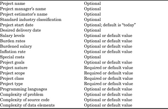
If the estimating tool includes sizing logic, it can produce project size estimates that the users can either accept or adjust as appropriate. However, in order to generate an accurate cost estimate, the commercial software estimating tools utilize the kinds of size information shown in Table 9.21, regardless of whether the information is generated by the tool itself, is supplied by the user, or both in some cases (the tool predicts a suggested value and the user may adjust or replace the value if desired).

Software projects have many different kinds of deliverable artifacts besides the code itself, and accurate software cost estimates must include these non-code deliverables in order to ensure that the estimate is complete and useful.

Similar kinds of information are required for estimating other types of projects besides software projects. For example, if you were working with an architect on designing and building a custom home, you would have to provide the architect with some basic information on how many square feet you wanted the house to be. A luxury house with 6000 square feet of living space and a three-car garage will obviously be more expensive to construct than a starter home with 1500 square feet and a one-car carport.

TABLE 9.21 Predicted Size Information or User-Supplied Size Information

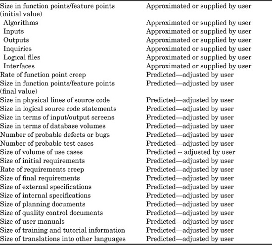
Strengths and Weaknesses of Software Size Metrics

Unfortunately, the current conflict between rival metrics enthusiasts is slowing down progress in software sizing and estimating technology. In fact, the conflicts are so sharp that it often escapes notice that none of the currently available metrics can measure every important aspect of software.

The LOC-metrics have major problems for dealing with non-coding activities and for comparisons between unlike programming languages. Also, for certain languages, such as Visual Basic and its competitors, coding is only one way of developing applications. The LOC-metric has no relevance for software constructed using button control and pull-down menus.

The function point metrics in all varieties have problems with counting precision for any specific variant, and even larger problems with converting data between variants. There are also severe problems across all function point variants for very small projects where certain constants in the counting rules tend to artificially inflate the results below about 15 function points.

The object-oriented (OO) metrics are totally devoid of relevance for non-OO projects, and do not seem to deal with OO quality or defect rates. The OO metrics are also lacking the ability to predict the non-code aspects of software development. There are no known conversion rules between the OO metrics and the other size metrics.

The more obscure size metrics, such as the Halstead software-science metrics, are yet additional variants. The original studies for software science appear to have methodological flaws, and the volume of published data for software-science metrics is only marginally greater than zero.

In addition to basic size metrics, there are also metrics that are used for size adjustments, such as complexity. Of the 24 known forms of complexity that influence software projects, only two (cyclomatic and essential complexity) have significant literature. Unfortunately, many of the more critical complexity metrics have no literature in a software context, although psychologists and linguists deal with them.

There are also attempts to use “natural” metrics, such as number of pages of specifications or number of staff hours. Here, too, there are problems with accuracy and with data conversion from these metrics to any other known metric.

There are no known metrics of any form that can deal with the topic of the size of databases, nor with the important topic of data quality. Fundamental metrics research is needed in the database arena.

The explosive growth of web-based applications brings up another metrics gap: the ability to measure web content in terms of size, cost, and quality.

The literature on metrics conversion between the competing function point methods, the competing LOC methods, and the other methods (object-oriented metrics, software-science metrics, etc.) is only marginally better than a null set.

The following would be advantageous to the software industry overall:

A complete analysis of the strengths and weaknesses of all current metrics

A concerted effort to develop industrial-strength function metrics that can support all software activities

Development of a standard activity table for the major software activities, so that such terms as requirements or design have the same general meaning and include the same task sets

The elimination of the scores of minor function point variants with few users and little published data or, at the very least, publication of conversion rules between minor variants and major function point forms

A consistent set of source code counting rules that could be applied to all programming languages, including visual languages

Development of a data point metric derived from the structure of function point metrics, but aimed at quantifying the sizes of databases, repositories, data warehouses, and flat files

Development of metrics for dealing with the size and quality of web content in the forms of images, sounds, animation, links, etc.

If multiple and conflicting metrics continue to be used, then metrics-conversion tools should be added to the software management toolkit to facilitate international comparisons when the data originates using multiple metrics.

The eventual goal of metrics research would be to facilitate the sizing and estimating of complex hybrid systems where software, microcode, hardware, data, and service components all contribute to the final constructed artifact.

What would probably be of immediate use to the software industry would be to publish formal rules for conversion logic between the major competing metrics. Even better would be automated metrics conversion tools that could handle a broad range of current metrics problems, such as the following:

Rules for size conversion between IFPUG Versions 3.4 and 4.1 counting methods

Rules for size conversion between IFPUG, COSMIC, NESMA, and Mark II counting methods

Rules for size conversion between source code and function point metrics

Rules for code size conversion between SPR and SEI code counting methods

Rules for size conversion between object-oriented metrics and any other metric

Rules for size conversion between two unlike programming languages

As an experiment, the author has constructed a prototype metric conversion tool that can handle some of these conversion problems, such as conversion between the SPR logical statement counts and the SEI physical line counts for selected programming languages.

While the prototype demonstrates that automatic conversion is feasible, the total number of variations in the industry is so large that a full-scale metric-conversion tool that can handle all common variants would be a major application in its own right. For such a tool to stay current, it would be necessary to keep it updated on an almost monthly basis, as new languages and new metrics appear.

Summary and Conclusions

Software sizing is a critical but difficult part of software cost estimating. The invention of function point metrics has simplified the sizing of non-code artifacts, such as specifications and user documents, but sizing is still a complicated and tricky undertaking.

While function points in general have simplified and improved software sizing, the unexpected fragmentation of function point metrics into more than 38 variants has added an unnecessary amount of confusion to the task of sizing, without contributing much in terms of technical precision.

The most accurate and best method for software sizing is to keep very good historical data of the sizes of software project deliverables. This way it will be possible to use the known sizes of artifacts from completed projects as a jumping-off place for predicting the sizes of similar artifacts for projects being estimated.

References

Abran, A., and P. N. Robillard: “Function Point Analysis: An Empirical Study of Its Measurement Processes,” IEEE Transactions on Software Engineering, 22(12):895–909 (1996).

Abrieu, Fernando Brito e: “An email information on MOOD,” Metrics News, Otto-von-Guericke-Univeersitaat, Magdeburg, 7(2):11 (1997).

Albrecht, A. J.: “Measuring Application Development Productivity,” Proceedings of the Joint IBM/SHARE/GUIDE Application Development Symposium, October 1979, reprinted in Programming Productivity—Issues for the Eighties by Capers Jones, IEEE Computer Society Press, New York, 1981.

Artow, J. and I Neustadt: UML and the Unified Process, Addison-Wesley, Boston, Mass., 2000.

———: AD/M Productivity Measurement and Estimate Validation, IBM Corporation, Purchase, N.Y., 1984.

Boehm, Barry: Software Engineering Economics, Prentice-Hall, Englewood Cliffs, N.J., 1981.

Booch, Grady, Ivar Jacobsen, and James Rumbaugh: The Unified Modeling Language User Guide, Second Edition, Addison-Wesley, Boston, Mass., 2005.

Bogan, Christopher E., and Michael J. English: Benchmarking for Best Practices, McGraw-Hill, New York, 1994.

Brown, Norm (ed.): The Program Manager’s Guide to Software Acquisition Best Practices, Version 1.0, U.S. Department of Defense, Washington, D.C., 1995.

Chidamber, S. R., D. P. Darcy, and C. F. Kemerer: “Managerial Use of Object Oriented Software Metrics,” Working Paper no. 750, Joseph M. Katz Graduate School of Business, University of Pittsburgh, Pittsburgh, Pa., November 1996.

———, and C. F. Kemerer: “A Metrics Suite for Object Oriented Design,” IEEE Transactions on Software Engineering, 20:476–493 (1994).

Cockburn, Alistair: Agile Software Development, Addison-Wesley, Boston, Mass., 2001.

Cohn, Mike: Agile Estimating and Planning, Prentice-Hall PTR, Englewood Cliffs, N.J., 2005.

———: User Stories Applied: For Agile Software Development, Addison-Wesley, Boston, Mass., 2004.

DeMarco, Tom: Controlling Software Projects, Yourdon Press, New York, 1982.

———: Why Does Software Cost So Much?, Dorset House, New York, 1995.

Department of the Air Force: Guidelines for Successful Acquisition and Management of Software Intensive Systems, vols. 1 and 2, Software Technology Support Center, Hill Air Force Base, Utah, 1994.

Dreger, Brian: Function Point Analysis, Prentice-Hall, Englewood Cliffs, N.J., 1989.

Fenton, Norman, and Shari Lawrence Pfleeger: Software Metrics—A Rigorous and Practical Approach, Second Edition, IEEE Press, Los Alamitos, Calif., 1997.

Fetchke, Thomas, Alain Abran, Tho-Hau Nguyen: Mapping the OO-Jacobsen Approach into Function Point Analysis, University du Quebec a Montreal, Software Engineering Management Research Laboratory, 1997.

Fuqua, Andrew M.: Using Function Points in XP—Considerations, Springer Berlin/Heidelberg, 2003.

Galea, R. B.: The Boeing Company: 3D Function Point Extensions, V2.0, Release 1.0, Boeing Information Support Services, Seattle, Wash., June 1995.

Gamma, Erich, Richard Helm, Ralph Johnson, and John Vlissides: Design Patterns: Elements of Reusable Object Oriented Design, Addison-Wesley, Boston Mass., 1995.

Garmus, David, and David Herron: Measuring the Software Process: A Practical Guide to Functional Measurement, Prentice-Hall, Englewood Cliffs, N.J., 1995.

Grady, Robert B.: Practical Software Metrics for Project Management and Process Improvement, Prentice-Hall, Englewood Cliffs, N.J., 1992.

———, and Deborah L. Caswell: Software Metrics: Establishing a Company-Wide Program, Prentice-Hall, Englewood Cliffs, N.J., 1987.

Halstead, Maurice H.: Elements of Software Science, Elsevier North Holland, NY, 1977.

Howard, Alan (ed.): Software Metrics and Project Management Tools, Applied Computer Research (ACR), Phoenix, Ariz., 1997.

IFPUG Counting Practices Manual, Release 3, International Function Point Users Group, Westerville, Ohio, April 1990.

———, Release 4, International Function Point Users Group, Westerville, Ohio, April 1995.

International Organization for Standards, ISO 9000 / ISO 14000 (http://www.iso.org/iso/en/iso9000-14000/index.html).

Jones, Capers: SPQR/20 Users Guide, Software Productivity Research, Cambridge, Mass., 1986.

———: Critical Problems in Software Measurement, Information Systems Management Group, 1993a.

———: Software Productivity and Quality Today—The Worldwide Perspective, Information Systems Management Group, 1993b.

———: Assessment and Control of Software Risks, Prentice-Hall, Englewood Cliffs, N.J., 1994.

———: New Directions in Software Management, Information Systems Management Group,

———: Patterns of Software System Failure and Success, International Thomson Computer Press, Boston, 1995.

———: Applied Software Measurement, Second Edition, McGraw-Hill, New York, 1996a.

———: Table of Programming Languages and Levels (8 Versions from 1985 through July 1996), Software Productivity Research, Burlington, Mass., 1996b.

———: The Economics of Object-Oriented Software, Software Productivity Research, Burlington, Mass., April 1997a.

———: Software Quality—Analysis and Guidelines for Success, International Thomson Computer Press, Boston, 1997b.

———: The Year 2000 Software Problem—Quantifying the Costs and Assessing the Consequences, Addison-Wesley, Reading, Mass., 1998.

Kan, Stephen H.:, Addison-Wesley Longman, Boston, Mass., 2003.

Kemerer, C. F.: “Reliability of Function Point Measurement—A Field Experiment,” Communications of the ACM, 36:85–97 (1993).

Love, Tom: Object Lessons, SIGS Books, New York, 1993.

McCabe, Thomas J.; A Complexity Measure; IEEE Transactions on Software Engineering; Vol. SE-2, No. 4; 1976; pg. 308-318.

McConnell, Steve: Software Estimating: Demystifying the Black Art, Microsoft Press, Redmond, WA; 2006.

Marciniak, John J. (ed.): Encyclopedia of Software Engineering, vols. 1 and 2, John Wiley & Sons, New York, 1994.

McCabe, Thomas J.: “A Complexity Measure,” IEEE Transactions on Software Engineering, (December 1976) pp. 308–320.

Muller, Monika, and Alain Abram (eds.): Metrics in Software Evolution, R. Oldenbourg Vertag GmbH, Munich, 1995.

Oman, Paul, and Shari Lawrence Pfleeger (eds.): Applying Software Metrics, IEEE Press, Los Alamitos, Calif., 1996.

Pressman, Roger: Software Engineering – A Practitioner’s Approach, Sixth Edition, McGraw-Hill, New York, 2005.

Putnam, Lawrence H.: Measures for Excellence—Reliable Software on Time, Within Budget, Yourdon Press/Prentice-Hall, Englewood Cliffs, N.J., 1992.

———, and Ware Myers: Industrial Strength Software—Effective Management Using Measurement, IEEE Press, Los Alamitos, Calif., 1997.

Rethinking the Software Process, CD-ROM, Miller Freeman, Lawrence, Kans., 1996. (This CD-ROM is a book collection jointly produced by the book publisher, Prentice-Hall, and the journal publisher, Miller Freeman. It contains the full text and illustrations of five Prentice-Hall books: Assessment and Control of Software Risks by Capers Jones; Controlling Software Projects by Tom DeMarco; Function Point Analysis by Brian Dreger; Measures for Excellence by Larry Putnam and Ware Myers; and Object-Oriented Software Metrics by Mark Lorenz and Jeff Kidd.)

Shavisprasad Koirala: “How to Prepare Quotations Using Use Case Points” (http://www.codeproject.com/gen/design//usecasepoints.asp).

Shepperd, M.: “A Critique of Cyclomatic Complexity as a Software Metric,” Software Engineering Journal, 3:30–36 (1988).

St-Pierre, Denis, Marcela Maya, Alain Abran, and Jean-Marc Desharnais: Full Function Points: Function Point Extensions for Real-Time Software, Concepts and Definitions, TR 1997-03, University of Quebec, Software Engineering Laboratory in Applied Metrics (SELAM), March 1997.

Stukes, Sherry, Jason Deshoretz, Henry Apgar, and Ilona Macias: Air Force Cost Analysis Agency Software Estimating Model Analysis—Final Report, TR-9545/008-2, Contract F04701-95-D-0003, Task 008, Management Consulting & Research, Inc., Thousand Oaks, Calif., September 1996.

Symons, Charles R.: Software Sizing and Estimating—Mk II FPA (Function Point Analysis), John Wiley & Sons, Chichester, U.K., 1991.

———: “ISMI—International Software Metrics Initiative—Project Proposal” (private communication), June 15, 1997.

———: “Software Sizing and Estimating: Can Function Point Methods Meet Industry Needs?” (unpublished draft submitted to the IEEE for possible publication), Guild of Independent Function Point Analysts, London, U.K., August 1997.

Whitmire, S. A.: “3-D Function Points: Scientific and Real-Time Extensions to Function Points,” Proceedings of the 1992 Pacific Northwest Software Quality Conference, June 1, 1992.

Zuse, Dr. Horst; Software Complexity: Measures and Methods; Walter de Gruyter, Berlin, 1990.