You can make your PivotTable chores quicker and easier by taking advantage of the buttons on the PivotTable toolbar. Most of these buttons give you one-click access to the most PivotTable features. You can also click the PivotTable button to display a list of commands available for your PivotTables.

Normally the PivotTable toolbar appears automatically when you create a PivotTable. When you click a cell outside the PivotTable, the PivotTable toolbar disappears, and it reappears when you click a cell within the PivotTable. However, you can also turn the PivotTable toolbar on and off by hand. For example, if your PivotTable report takes up all or most of the screen, you may prefer to turn off the PivotTable toolbar to prevent it from covering any data.

Here is a summary of the most useful PivotTable toolbar buttons; each button is described in more detail elsewhere in the book:

Button	Description
	Displays the AutoFormat dialog box (Chapter 6)
	Creates a PivotChart (Chapter 9)
	Hides the detail in a group (Chapter 4)
	Shows the detail in a group (Chapter 4); shows the underlying detail for a field or data value (Chapter 3)
	Refreshes the PivotTable (Chapter 3)
	Includes hidden data in totals (Chapter 8)
	Displays unique field values as you add items to the PivotTable (Chapter 2)
	Displays the PivotTable Field dialog box (Chapter 5)
	Toggles the PivotTable Field List on and off (Chapter 2)

Turn the PivotTable Toolbar On and Off

TURN OFF THE PIVOTTABLE TOOLBAR

Note

This chapter uses the Orders.xls and PivotTables.xls spreadsheets, available at www.wiley.com/go/pivottablesvb, or you can create your own sample database.

You can also click View→Toolbars→PivotTable, or right-click any toolbar or menu and then click PivotTable.

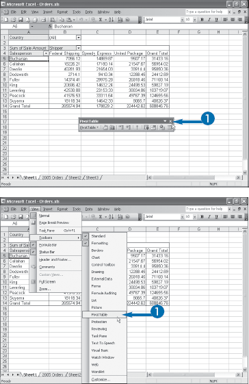
Excel turns off the PivotTable toolbar.

TURN ON THE PIVOTTABLE TOOLBAR

You can also right-click any toolbar or menu and then click PivotTable.

Excel turns on the PivotTable toolbar.

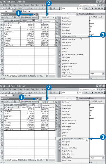
The buttons on the default PivotTable toolbar are very useful, but you may find that you do not use some of them very often. For example, if you never group your PivotTable data, then you will never need the Hide Detail and Show Detail buttons; see Chapter 4. You can make the PivotTable toolbar easier to work with by removing those buttons you do not use.

On the other hand, there may be PivotTable features that you use quite often, but the PivotTable does not offer a button. For example, if you often use the PivotTable and PivotChart Wizard, you have to click PivotTable→PivotTable Wizard to run it. You can save a click by adding a button for this command directly to the toolbar.

Here is a summary of the most useful extra PivotTable toolbar buttons that you can add; each button is described in more detail elsewhere in the book:

Button	Description
	Ungroups PivotTable data (Chapter 4)
	Groups PivotTable data (Chapter 4)
	Starts the PivotTable and PivotChart Wizard (Chapter 2)
	Shows pages in separate worksheets (Chapter 4)
	Refreshes all PivotTables in the current workbook (Chapter 3)
	Automatically generates GETPIVOTDATA() formulas (Chapter 10)
	Displays properties associated with an OLAP cube (Chapter 11)

Customize the PivotTable Toolbar

REMOVE A BUTTON FROM THE PIVOTTABLE TOOLBAR

Excel displays a list of all the available PivotTable toolbar buttons.

Excel removes the check mark from beside the button and updates the toolbar.

ADD A BUTTON TO THE PIVOTTABLE TOOLBAR

Excel displays a list of all the available PivotTable toolbar buttons.

Excel displays a check mark beside the button and updates the toolbar.

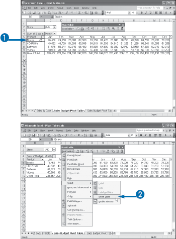
In many of the tasks in this book, you will apply formatting or settings to some or all of the PivotTable's cells, or you will perform some action on some or all of the PivotTable's cells. Before you can do any of this, however, you must first select the cell or cells you want to work with. You can speed up your PivotTable work considerably by becoming familiar with the various methods that Excel offers for selecting elements in a PivotTable report.

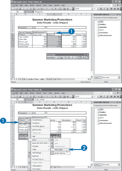
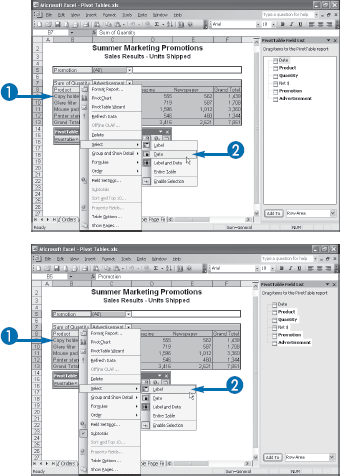
If you are familiar with Excel, then you probably already know the basic techniques for selecting cells. For example, you select a single cell by clicking it, and you select a range by dragging your mouse from the top-left corner of the range to the bottom-right corner. You can also select random cells by holding down Ctrl and clicking the cells you want. You can use all the standard techniques to select cells within a PivotTable report. However, Excel also offers several methods that are unique to PivotTables. For example, you can select one or more row or column fields, just the PivotTable labels, just the PivotTable data, or the entire table. Excel also offers handy toolbar buttons for most of these techniques, so you can customize the PivotTable toolbar for one-click access to PivotTable selection techniques.

Select PivotTable Items

SELECT A ROW OR COLUMN FIELD

The mouse pointer changes to a black, downward-pointing arrow.

For a row, move the mouse pointer just to the left of the row label. The mouse pointer changes to a right-pointing arrow.

Excel selects the column.

From the keyboard, use the arrow keys to move the cursor into the label of the column or row.

SELECT THE ENTIRE PIVOTTABLE

You can also move the mouse pointer to the top or left edge of the upper-left PivotTable cell (the pointer changes to

Excel selects the entire table.

To select all the row and column fields, click any cell in a row or column field and then press Ctrl+Shift+8.

SELECT DATA ONLY

Excel selects just the PivotTable's data area.

If you select a field instead of the entire table, click PivotTable→Select→Data to select just that field's data.

SELECT LABELS ONLY

Excel selects just the PivotTable's labels.

If you select a field instead of the entire table, click PivotTable→Select→Label to select just that field's label.

Extra

You can make your PivotTable selection chores even easier by incorporating one or more extra toolbar buttons on the PivotTable toolbar. Excel offers extra buttons for the Data, Label, and Label and Data commands that appear when you click PivotTable→Select in the PivotTable toolbar.

Select View→Toolbars→Customize to display the Customize dialog box. Click the Commands tab and then click Data in the Categories list. Scroll down the Commands list until you see the following buttons:

Button	Description
	Selects the PivotTable labels.
	Selects the PivotTable data.
	Selects a field's label and data when the field's label or data is currently selected.

Drag the button you want and drop it on the PivotTable toolbar. When you are finished, click Close to shut down the Customize dialog box.

After you have completed your PivotTable, the resulting report is not set in stone. You will see in Chapter 4 and in other parts of this book that you can change the PivotTable view, format the PivotTable cells, add custom calculations, and much more. You can also remove fields from the PivotTable report, as you learn in this task.

Removing a PivotTable field comes in handy when you want to work with a less detailed report. For example, suppose your PivotTable report shows the sum of sales data from four items in the Region field — East, Midwest, South, and West — that appear in the row area. This data is broken down by fiscal quarter, where each item in the Quarter field appears in the column area. If you decide you want to simplify the report to show just the total for each region, then you need to remove the Quarter field from the PivotTable.

Remove a field from a PivotTable only if you are sure you will not need the field again in the future. You can always add fields back into the PivotTable report, but deleting a field and then adding it back again is inefficient. If you only want to take a field out of the PivotTable report temporarily, consider hiding the field; see the task "Hide Items in a Row or Column Field," in Chapter 4.

Similarly, you do not need to go through the process of removing a field if you know that the field has been removed from the original data source. Instead, refresh the PivotTable and Excel will remove the deleted field for you automatically; see the task "Refresh PivotTable Data," later in this chapter.

Remove a PivotTable Field

REMOVE A FIELD FROM THE PIVOTTABLE REPORT

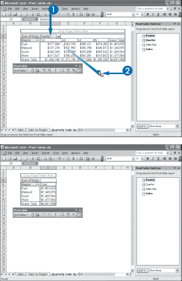
The mouse pointer changes to

Excel removes the field from the PivotTable report.

REMOVE A FIELD USING THE PIVOTTABLE WIZARD

Note

To learn how to display the Layout dialog box, see the task "Add Fields Using the PivotTable Wizard" in Chapter 2.

The mouse pointer changes to

Excel removes the field from the PivotTable diagram.

Excel removes the field from the PivotTable report.

Apply It

Removing fields is particularly handy when you work with multiple fields in a single area, as described in the tasks "Add Multiple Fields to the Row or Column Area," "Add Multiple Fields to the Data Area," and "Add Multiple Fields to the Page Area," later in this chapter. If you find that a PivotTable with multiple fields in one area is too confusing or too cumbersome to manipulate, removing one or more of those fields can simplify the layout and help you get more out of your PivotTable.

It is worth noting here, as well, that you cannot delete part of a field. For example, if you have a Region field, you cannot delete the Midwest item. If you select a cell, row, or column within the PivotTable and press Delete, Excel displays an error message telling you that you cannot delete part of the PivotTable report. Again, it is possible to hide individual rows and columns within a PivotTable; see the task "Hide Items in a Row or Column Field" in Chapter 4.

Whether your PivotTable is based on financial results, survey responses, or a database of collectibles such as books or DVDs, the underlying data is probably not static. That is, the data changes over time as new results come in, new surveys are undertaken, and new items are added to the collection. You can ensure that the data analysis represented by the PivotTable remains up to date by refreshing the PivotTable, as shown in this task.

Refreshing the PivotTable means rebuilding the report using the most current version of the source data. However, this is not the same as running the PivotTable and PivotChart Wizard over again, as described in Chapter 2 in the task "Re-create an Existing PivotTable." Instead, when you refresh a PivotTable, Excel keeps the report layout as is and simply updates the data area calculations with the latest source data. Also, depending on the type of source data you are using, Excel will remove from the report any fields that have been deleted from the source data, and it will display in the PivotTable Field List any new fields that have been added to the source data.

Excel offers two methods for refreshing a PivotTable: manually and automatically. A manual refresh is one that you perform yourself, usually when you know that the source data has changed, or if you simply want to be sure that the latest data is reflected in your PivotTable report. An automatic refresh is one that Excel handles for you. For PivotTables based on Excel ranges or lists, you can tell Excel to refresh a PivotTable every time you open the workbook that contains the report.

Refresh PivotTable Data

REFRESH DATA MANUALLY

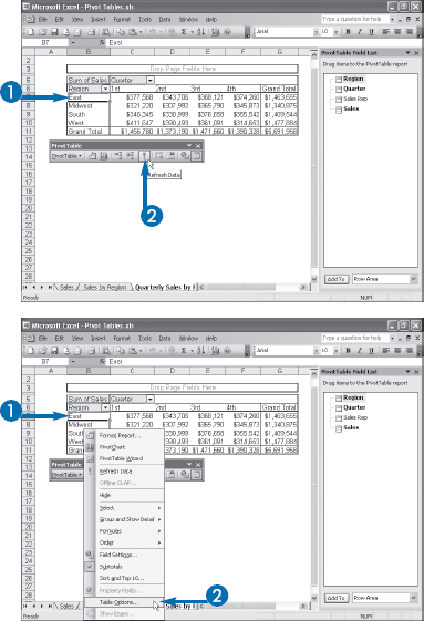
You can also select PivotTable→Refresh Data on the PivotTable toolbar. Alternatively, click Data→Refresh Data.

To update every PivotTable in the current workbook, click the Refresh All button (

Excel updates the PivotTable data.

REFRESH DATA AUTOMATICALLY

The PivotTable Options dialog box appears.

Excel applies the refresh options.

Apply It

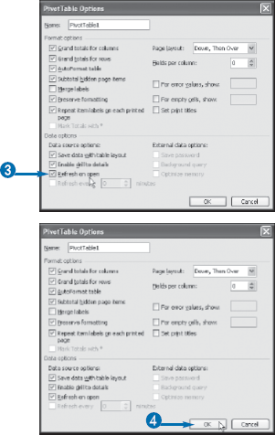
For certain types of source data, you can set up a schedule that automatically refreshes the PivotTable at a specified interval. This is useful when you know the source data changes frequently and you do not want to be bothered with constant manual refreshes.

Click any cell inside the PivotTable, and then click PivotTable→Table Options. In the PivotTable Options dialog box, examine the "Refresh every" check box. If this check box is not enabled, it means your source data does not support automatic refreshing at preset intervals. For example, this check box is not enabled when you use an Excel range or list as the data source. However, for data that comes from other types of data sources, particularly external data, this check box is enabled. See Chapter 10 to learn how to build a PivotTable from data sources other than Excel ranges and lists. If you want to refresh the PivotTable automatically at a specified interval, select "Refresh every" (

Note, however, that you might prefer not to have the source data updated too frequently. Depending on where the data resides and how much data you are working with, the refresh could take some time, which will slow down the rest of your work.

The main advantage to using PivotTables is that they give you an easy method for summarizing large quantities of data into a succinct report for data analysis. PivotTables show you the forest instead of the trees. However, there may be times when you need to see some of the trees that comprise the forest. For example, if you are studying the results of a marketing campaign, your PivotTable may show you the total number of mouse pads sold as a result of a direct marketing piece. However, what if you want to see the details underlying that number? If your source data contains hundreds or thousands of records, you would need to filter the data in some way to see just the records you want.

Fortunately, Excel gives you an easier way to do this by allowing you to directly view the details that underlie a specific data value. This is called drilling down to the details. When you drill down into a specific data value in a PivotTable, Excel returns to the source data, extracts the records that comprise the data value, and then displays the records in a new worksheet. For a PivotTable based on a range or list, this extraction takes but a second or two, depending on how many records there are in the source data.

This task shows you how easy it is to drill down into your PivotTable data. In fact, it is so easy and so useful, that many people find themselves frequently drilling down to peek behind the data. Unfortunately, because Excel creates a new worksheet each time, this often results in a workbook that is cluttered with many extra worksheets. Therefore, this task also shows you how to delete the detail worksheets.

Display the Details Behind PivotTable Data

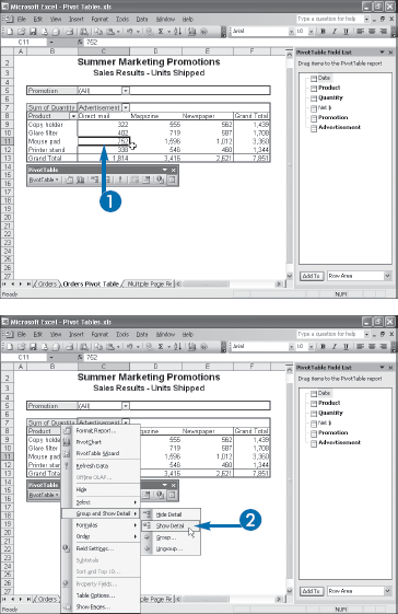
You can also double-click the data value or click the Show Detail button (

Excel displays the underlying data in a new worksheet.

DELETE THE DETAIL WORKSHEET

Excel displays a dialog box asking you to confirm the deletion.

Excel deletes the worksheet.

Extra

When you attempt to drill down to a data value's underlying details, Excel may display the error message "Cannot change this part of a PivotTable report." This error means that the feature that normally enables you to drill down has been turned off. To turn this feature back on, click PivotTable→Table Options to display the PivotTable Options dialog box. Select "Enable drill to details" (

The opposite situation occurs when you distribute the workbook containing the PivotTable and you do not want the other users drilling down and cluttering the workbook with detail worksheets. In this case, click PivotTable→Table Options to display the PivotTable Options dialog box, deselect "Enable drill to details" (

There may be times when you want to see all of a PivotTable's underlying source data. If the source data is a range or list in another worksheet, then you need only display that sheet. If the source data is not so readily available, however, then Excel gives you an easy way to view all the underlying data. Click the PivotTable's Grand Total cell and then click PivotTable→Group and Show Detail→Show Detail.

Excel charts are a great way to analyze data because they enable you to visualize the numbers and see the relationships between different aspects of the data. This is particularly useful in a PivotTable because it is often necessary to visualize the relationship between different columns or different rows. In Chapter 9, you learn how to create a PivotChart. However, if you just need a simple chart, or if you avoid the limitations that are inherent with a PivotChart, you can create a regular chart using the PivotTable data, as you learn in this task.

If you try to create a chart directly from a PivotTable, Excel will create a PivotChart. To create a regular chart from a PivotTable, you must first copy the PivotTable data that you want to graph, and then paste the data into another part of the worksheet. You can then build your chart using this copied data. In this case, you run through the various steps provided by the Chart Wizard to specify the chart type, chart options, and chart location.

Note, though, that this method produces a static chart. This means that if your PivotTable data changes, your chart does not change automatically. Instead, you need to re-create your chart from scratch. However, it is possible to create a dynamic chart that changes whenever your PivotTable does. See the tip on page 39 for details.

Create a Chart from PivotTable Data

CREATE A COPY OF THE PIVOTTABLE DATA

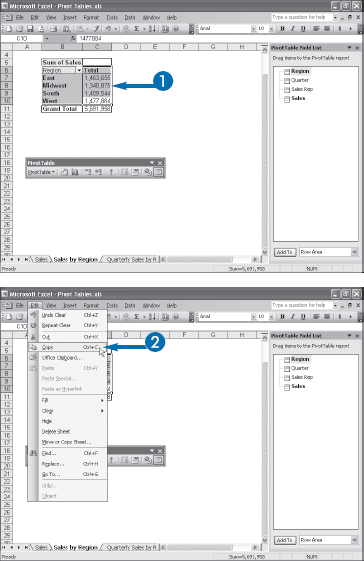
You can also press Ctrl+C or click the Copy button (

Excel copies the PivotTable data.

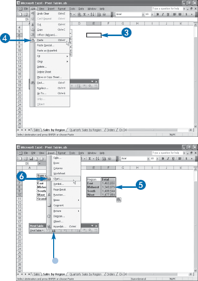
You can also press Ctrl+V or click the Paste button (

Excel pastes the copied PivotTable data.

CREATE THE CHART

The Chart Wizard's first dialog box appears.

Extra

PivotTables often result in large workbooks because Excel must keep track of a great deal of extra information to keep the PivotTable performance acceptable. In Chapter 4, you learn how to pivot the data, which means moving a field to a different area of the PivotTable; see the task "Move a Field to a Different Area". To ensure that the recalculation involved in pivoting happens quickly and efficiently, Excel maintains a copy of the source data in a special memory area called the pivot cache.

When you copy a PivotTable and then paste it, Excel also pastes the pivot cache. This is wasteful because the pasted data does not and can not make use of the pivot cache. To avoid this, you should tell Excel to paste only the values from the PivotTable. To do this, follow the steps in the task "Convert a PivotTable to Regular Data," later in this chapter.

As you learn in Chapter 9, a PivotChart, although very similar to a regular Excel chart, comes with a number of limitations on chart types, layout, and formatting; see the section "Understanding PivotChart Limitations". A PivotChart also comes with its own pivot cache, a concept you learned about in the tip on the previous page. This means that PivotCharts can use up a great deal of memory and can greatly increase the size of a workbook.

If you simply want to visualize your data, you can avoid the limitations and resource requirements of a PivotChart by creating a regular chart, instead. You do this by running the Chart Wizard on your copied PivotTable data. With a regular chart, you have access to all the available charting features, so you can use all the options presented by the Chart Wizard to construct your graph.

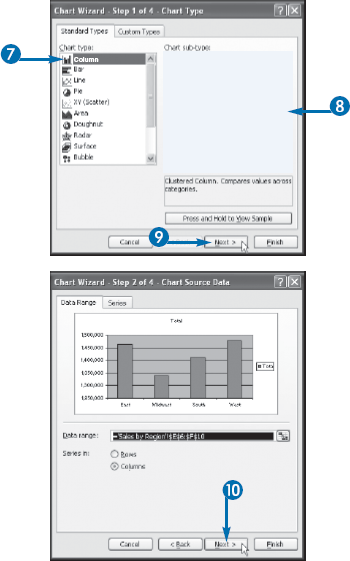
The second Chart Wizard dialog box appears.

The third Chart Wizard dialog box appears.

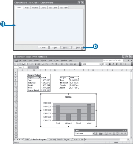
If you want to create the chart on a separate worksheet, click Next and then click "As new sheet."

Excel creates the chart.

Apply It

The chart you learn how to create in this task is static, so whenever your PivotTable gets new values, you must re-create the chart from scratch. This is useful for PivotTables that do not change fields, items, or data. However, if you have a PivotTable that changes frequently, you might prefer to create a dynamic chart that updates automatically when changes occur in your PivotTable data.

To create a dynamic chart, use formulas instead of copy and paste to create a replica of the PivotTable data. That is, for each cell in the PivotTable that you want to use in your chart, create a formula in another cell that references the PivotTable cell. For example, in cell E6, enter the formula =B6 to reference the Region label; similarly, in cell F6, enter the formula =C6 to reference the Total label. Do the same for the data values. For example, in cell F7, enter the formula =C7. When you are done, you should have the same labels and values in a replica of the PivotTable. You can then base your chart on this replicated data. Because you are using formulas to reference the original data, any changes to the PivotTable will automatically be reflected in your chart.

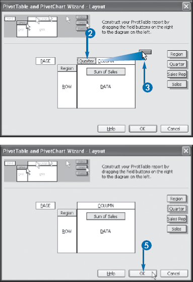
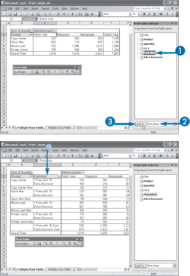
The PivotTables you have seen so far have been restricted to a single field in any of the four areas: row, column, data, and page. However, you are free to add multiple fields to any one of these areas. This is a very powerful technique because it allows you to perform further analysis of your data by viewing the data differently.

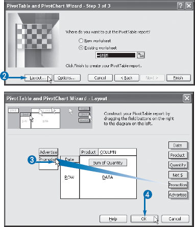
In this task you learn how to add multiple fields to a PivotTable's row and column areas. See the next tasks, "Add Multiple Fields to the Data Area" and "Add Multiple Fields to the Page Area," as well. Adding multiple fields to the row and column areas enables you to break down your data for further analysis. For example, suppose you are analyzing the results of a sales campaign that ran different promotions in several types of advertisements. A basic PivotTable might show you the sales for each Product (the row field) according to the Advertisement in which the customer reported seeing the campaign (the column field). You might also be interested in seeing, for each product, the breakdown in sales for each promotion. You can do that by adding the Promotion field to the row area, as you see in the example used in this task.

Even more powerfully, after you add a second field to the row or column area, you can change the field positions to change the view, as described in Chapter 4 in the task "Change the Order of Fields within an Area." Note that the field in the row or column area that is closest to the data area is called the inner field and the field furthest from the data area is called the outer field.

Add Multiple Fields to the Row or Column Area

USE THE PIVOTTABLE FIELD LIST

USE THE PIVOTTABLE WIZARD

The PivotTable and PivotChart Wizard appears.

The Layout dialog box appears.

Excel adds the field to the PivotTable.

Extra

You can also add a field to the row or column area of a PivotTable by dragging. In the PivotTable Field List, click and drag the field you want to add. As you move the field into the PivotTable, the mouse pointer changes depending on the PivotTable area over which it is hovering:

Button	Description
	Mouse pointer for the row area.
	Mouse pointer for the column area.

When you see one of these pointers, dropping the field means that Excel adds the field to that area of the PivotTable.

Note, too, that where you drop the field with the row or column area is significant. In the row area, for example, you can either drop the new field to the right or to the left of the existing field. If you drop it to the right, Excel displays each item in the original field broken down by the items in the new field. This is the situation in the final screen shot, above, where you see each item in the Product field broken down by the two items in the Promotion field. Conversely, if you drop the new field to the left of the existing field, Excel displays each item in the new field broken down by the items in the original field.

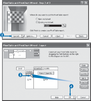
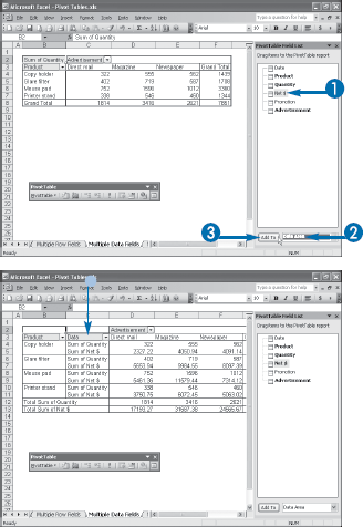
In this task you learn how to add multiple fields to the PivotTable's data area. See also the tasks "Add Multiple Fields to the Row and Column Area" and "Add Multiple Fields to the Page Area" in this chapter. Adding multiple fields to the data area enables you to see multiple summaries for enhancing your analysis. For example, suppose you are analyzing the results of a sales campaign that ran different promotions in several types of advertisements. A basic PivotTable might show you the sum of the Quantity sold (the data field) for each Product (the row field) according to the Advertisement in which the customer reported seeing the campaign (the column field). You might also be interested in seeing, for each product and advertisement, the net dollar amount sold. You can do that by adding the Net $ field to the data area, as you see in the example used in this task.

Even more powerfully, you are not restricted to using just sums in each data field. Excel enables you to specify a number of different summary functions in the data area, so you could apply a different function to each field. For example, you could view the sum of the Quantity field and the average of the Net $ field. You learn how to change the summary function in Chapter 7 in the task "Change the PivotTable Summary Calculation."

Add Multiple Fields to the Data Area

USE THE PIVOTTABLE FIELD LIST

USE THE PIVOTTABLE WIZARD

The PivotTable and PivotChart Wizard appears.

The Layout dialog box appears.

Excel adds the field to the PivotTable's data area.

Extra

You can also add a field to the PivotTable's data area by dragging. In the PivotTable Field List, click and drag the field you want to add. As you move the field into the PivotTable's data area, the mouse pointer changes to the data area mouse pointer (

When you see this pointer, drop the field to add it to the PivotTable's data area.

In the task "Remove a PivotTable Field," earlier in this chapter, you learned that you can delete a field from any PivotTable area by dragging the field's button and dropping it outside of the PivotTable. However, this technique does not work when you have multiple fields in the data area because Excel replaces the original field button with a Data button. Dragging this button off the PivotTable means that you remove all the data fields. To delete one of multiple fields in the data area, click PivotTable→PivotTable Wizard and then click Layout to display the Layout dialog box. Drag the data field you want to remove off the PivotTable diagram, and then click OK.

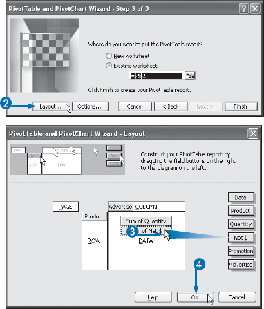
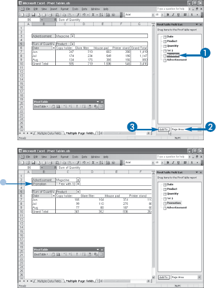
In this task you learn how to add multiple fields to the PivotTable's page area. See also the previous tasks, "Add Multiple Fields to the Row and Column Area" and "Add Multiple Fields to the Data Area." Adding multiple fields to the page area enables you to apply multiple filters to the PivotTable to enhance your analysis. For example, suppose you are analyzing the results of a sales campaign that ran different promotions in several types of advertisements. A basic PivotTable might show you the sum of the Quantity sold (the data field) for each Product (the column field) by Date (the row field), with a filter for the type of Advertisement (the page field). You might also be interested in filtering the data even further to show specific Promotion items. You can do that by adding the Promotion field to the page area, as you see in the example used in this task.

To get the most out of this technique, you need to know how to use a page area field to filter the data shown in a PivotTable. For example, you could use the Advertisement field to display the PivotTable results for just the Magazine item. With the Promotion field also added to the page area, you could filter the PivotTable even further to display just the results for the 1 Free with 10 item. In the Chapter 4 tasks "Display a Different Page" and "Change the Page Area Layout," you learn how to display different pages and how to reconfigure the page area layout, respectively.

Add Multiple Fields to the Page Area

USE THE PIVOTTABLE FIELD LIST

USE THE PIVOTTABLE WIZARD

The PivotTable and PivotChart Wizard appears.

The Layout dialog box appears.

Excel adds the field to the PivotTable's page area.

Extra

You can also add a field to the PivotTable's page area by dragging. In the PivotTable Field List, click and drag the field you want to add. As you move the field into the PivotTable's page area, the mouse pointer changes to the page area mouse pointer (

When you see this pointer, drop the field to add it to the PivotTable's page area.

Earlier you learned that the order of the fields with the PivotTable's row and column areas is important because it changes how Excel breaks down the data; see the task "Add Multiple Fields to the Row and Column Area," earlier in this chapter. The order of the fields in the page area is not important because the resulting filter is the same. For example, suppose you have a collection of shirts and you want to see only those that are white and short-sleeved. You could do this by first pulling out all the white shirts and then going through those to find all the short-sleeved ones. However, you get the same result if you first take out all the short-sleeved shirts and then find all of those that are white.

When you analyze data, it is often important to involve other people in the process. For example, you might want to have other people help with some or all of the analytical tasks. Similarly, you might want to share your results with other interested parties. If the other people have Excel, you can share the workload or the results simply by sending each person a copy of the workbook that contains the PivotTable. However, although Excel is extremely popular, not everyone uses it.

Whether you are sharing the work or the results, a related problem involves updates to the PivotTable data. You know you can always refresh the PivotTable to see the latest data; see the task "Refresh PivotTable Data," earlier in this chapter. However, it is inconvenient to have to send out a new copy of the workbook each time you update the PivotTable.

You can solve both problems by placing your PivotTable on a Web page, either on the Internet or on your corporate intranet site. After the PivotTable is in Web page format, anyone — even people who do not use Excel — can view the PivotTable. It is also possible to set up the Web page version of the PivotTable to be updated automatically whenever you save the original workbook, so other people always see the latest data. Finally, you can also create interactive PivotTables, which means that other people can work with the PivotTable within the Web browser. This task shows you the steps involved in publishing a PivotTable to a Web page.

Publish a PivotTable to a Web Page

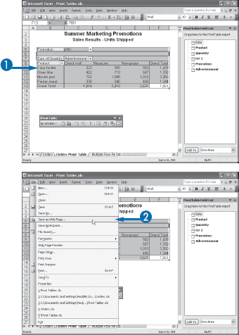
The Save As dialog box appears.

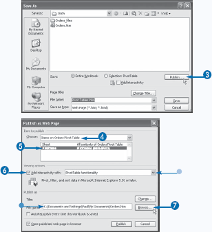
The Publish as Web Page dialog box appears.

The Publish As dialog box appears.

Apply It

You can tell Excel to add a title to the published PivotTable. This title appears in the Web page as text just above the PivotTable. To specify a title, click "Change in the Publish as Web Page dialog box" to display the Set Title dialog box. Type the title that you want to appear over the PivotTable and then click OK to return to the Publish as Web Page dialog box.

To ensure that the Web page version of your PivotTable is always up to date, you can tell Excel to update it for you automatically. In the Publish as Web Page dialog box, select "AutoRepublish every time this workbook is saved" (

When publishing a PivotTable, it is important to choose the proper location for the published Web page and its associated files. If you will be putting the PivotTable Web page on an Internet site, you should save the Web page to whatever folder you use for your other Web site files, which will likely be a subfolder of My Documents. If you will be putting the PivotTable Web page on your corporate intranet site, you should save the Web page to an appropriate network folder. Ask your system administrator for the correct folder and whether you need a username and password.

After you publish an Internet-based PivotTable Web page to your computer, you must then use an FTP utility or similar program to upload the Web page and its associated files to your directory on the Web server. You can save this extra step by specifying the particulars of your FTP sites within Excel, as described in the tip on the following page.

Note

When typing a name for the Web page, do not use spaces and make sure the name ends with either .htm or .html.

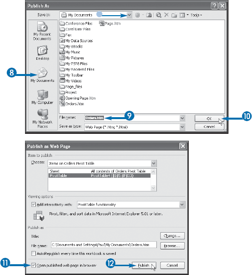
Excel returns you to the Publish as Web Page dialog box.

Excel publishes the PivotTable to the Web page.

If you are running Windows XP Service Pack 2 or later, Internet Explorer warns you that it has prevented the file from showing active content.

Internet Explorer displays a dialog box asking if you are sure you want to run the active content.

Internet Explorer displays the PivotTable on the Web page.

Apply It

When you publish a PivotTable (or any Excel data) to a Web page, Excel creates a subfolder named Filename_files, where Filename is the name you give to the Web page file, minus the extension. Excel uses this folder to hold support files for the Web page. For a PivotTable, you see two extra files: filelist.xml and a file with the name Filename _ID_cachedata001.xml, where Filename is the name of the Web page file and ID is a random 5-digit number.

If you prefer to keep all the files in a single folder — for example, to make it easier to copy the files to your Web site — you can tell Excel not to create the subfolder. Click Tools→Options, click the General tab, click Web Options, click the Files tab, and then deselect "Organize supporting files in a folder" (

To specify an FTP site for uploading, display the Save As dialog box, click Add/Modify FTP Locations in the Save in list, type the site address and your username and password, and then click Add.

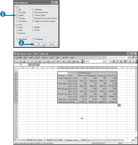
One of the major drawbacks of PivotTables is that they often require an inordinate amount of system resources. For example, it is not unusual to have source data that contains a large number of records or to have a PivotTable that is itself quite large and uses multiple fields in one or more areas. In such cases, the workbook containing the PivotTable can become huge and the memory used by Excel to store PivotTable data for faster performance can become excessive.

In situations where you need to manipulate the PivotTable frequently and where the source data changes, you have no choice but to put up with the burden that the PivotTable puts on your system. On the other hand, you may just be interested in the current PivotTable results and have no need to manipulate or refresh the data; similarly, you may not even need to keep the source data after you have built your PivotTable. In these scenarios, you can drastically reduce the resources used by the workbook by converting your PivotTable into regular data. When you have done that, you can delete the PivotTable — see the task "Delete a PivotTable," later in this chapter — and the source data, assuming the source data is an Excel range or list that you no longer need.

Convert a PivotTable to Regular Data

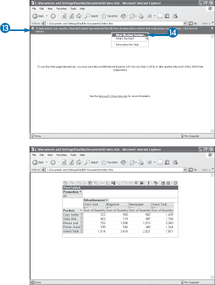
You can also press Ctrl+C or click the Copy button (

Excel copies the PivotTable data.

The Paste Special dialog box appears.

You can also press Ctrl+V or click the Paste button (

Excel pastes the PivotTable as regular data.

Apply It

The biggest problem that occurs when you convert a PivotTable to regular data is that Excel does not preserve any of your PivotTable formatting. See Chapter 5 to learn how to customize PivotTable fields. If you formatted your PivotTable with one of Excel's AutoFormats, then you can easily solve the problem: select the pasted data, click Format→AutoFormat, click the AutoFormat you want, and then click OK.

If you do not want to use an AutoFormat, Excel offers a simple way to at least preserve any numeric formats you applied to the PivotTable cells. In Chapter 5, see the task "Apply a Numeric Format to PivotTable Data." In the Paste Special dialog box, select "Values and number formats" (

If you just want to view the data and do not need to manipulate it in any way, you can preserve all your formatting by taking a "picture" of the PivotTable. Select the PivotTable, hold down Shift, and click Edit→Copy Picture. Select the cell where you want the picture to appear and then click Edit→Paste.

PivotTables are mostly useful in electronic format where you can perform the manipulations that you have learned about in this chapter, as well as change the PivotTable view to enhance your analysis of the data. See Chapter 4 to learn how to change the PivotTable view.

However, after you complete the PivotTable, you might want to preserve a hard copy by printing out the PivotTable report. You can use the printout to send a copy to another person, store the report in a file, or provide a backup if you lose the original electronic report or if the original report is no longer available.

Printing the PivotTable is also useful for documenting intermediate steps in the data analysis. If your analysis consists of four or five changes to the PivotTable, you could get a printout at each stage to document what you have done.

Printouts are also useful for comparing PivotTable results side by side. For example, you could construct the PivotTable using one layout and then print it out. You could then change the PivotTable layout and get a second printout. With the two printouts beside each other, you can then quickly scan the reports to compare them.

Print a PivotTable

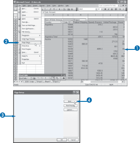
The Page Setup dialog box appears.

The Print dialog box appears.

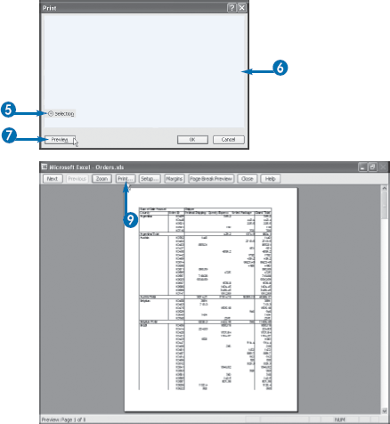
The Print Preview window appears.

Excel prints the PivotTable.

Extra

Excel offers a number of useful options for controlling the printout of a PivotTable. For example, if your PivotTable contains multiple row fields, it is often useful to display each item in the leftmost field on its own page. To set this up, right-click the leftmost field's button and then click Field Settings. Click Layout to display the PivotTable Field Layout dialog box, and then select "Insert page break after each item" (

Another useful printing option is to force Excel to print the row and column labels at the top of each printed page. To set this up, select the PivotTable and then click File→Print Area→Set Print Area. In the PivotTable toolbar, click PivotTable→Table Options to display the PivotTable Options dialog box. Select "Repeat item labels on each printed page" (

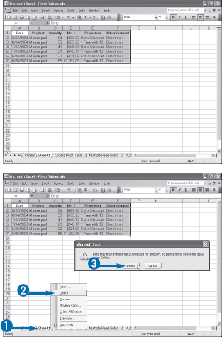
PivotTables are useful data analysis tools, and now that you are becoming comfortable with them, you may find that you use them quite often. This will give you tremendous insight into your data, but that insight comes at a cost: PivotTables are very resource-intensive, so creating many PivotTable reports can lead to large workbook file sizes and less memory available for other programs. You can reduce the impact that a large number of open PivotTables have on your system by deleting those reports that you no longer need.

Even if you create just a few PivotTables, you may find that you need them only temporarily. For example, you may just want to build a quick-and-dirty report to check a few numbers. Similarly, your source data may be preliminary, so you might want to create a temporary PivotTable for now, holding off on a more permanent version until your source data is complete. Finally, you might build PivotTable reports to send them to other people. When that is done, you might no longer need the reports yourself. For all these scenarios, you need to know how to delete a PivotTable report, and this task shows you how it is done.

Delete a PivotTable

Excel selects the PivotTable.

Excel deletes the PivotTable.

Apply It

If you create many temporary PivotTables, you should delete them to save system resources. However, this can become time-consuming if you do this quite often. To save time, use the following VBA macro (available in the sample PivotTables.xls workbook) to automatically delete the first PivotTable on the active worksheet:

Sub DeletePivotTable()
    Dim objPT As PivotTable, nResult As Integer
    '
    ' Work with the first PivotTable
    ' on the active worksheet
    Set objPT = ActiveSheet.PivotTables(1)
    '
    ' Confirm
    nResult = MsgBox("Are you sure you want " & _
              "to delete the PivotTable " & _
              "named " & objPT.Name & "?", vbYesNo)
    If nResult = vbYes Then
        '
        ' Select the PivotTable
        objPT.PivotSelect ""
        '
        ' Delete it
        Selection.Clear
    End If
End Sub