The most common method for building a PivotTable is to use data that exists in an Excel worksheet. You can make this task much easier by taking a few minutes to prepare your worksheet data for use in the PivotTable. Ensuring your data is properly prepared will also ensure that your PivotTable contains accurate and complete summaries of the data.
Preparing your worksheet data for use in a PivotTable is not difficult or time-consuming. At a minimum, you must ensure that the data is organized in a row-and-column format, with unique headings at the top of each column and accurate and consistent data — all numbers or all text — within each column. You also need to remove blank rows, turn off automatic subtotals, and format the data. In some cases, you may also need to add range names to the data, filter the data, and restructure the data so that worksheet labels appear within a column in the data. You may not need to perform all or even any of these tasks, but you should always ensure that your data is set up according to the guidelines you learn about in this task.
In the simplest case, Excel builds a PivotTable from worksheet data by finding the unique values in a specific column of data and summarizing — summing or counting — that data based on those unique values. For this to work properly, you need to ensure that your data is organized in such a way that Excel can find those unique values and compute accurate summaries.
You can perform some Excel tasks on data that is scattered here and there throughout a worksheet, but building a PivotTable is not one of them. To create a PivotTable, your data must be organized in a basic row-and-column format, where each column represents a particular aspect of the data, and each row represents an example of the data. For example, in a parts table, you might have columns for the part name, part number, and cost, and each row would display the name, number, and cost for an individual part.
The first row in your data must contain the headings that identify each column. Excel uses these headings to generate the PivotTable field names, so the headings must be unique and they must reside in a single cell.
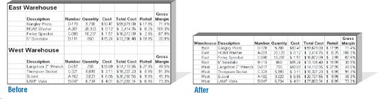
Many worksheets use labels — cells that contain descriptive text — as headings to differentiate one section of the worksheet from another. For example, a parts table might have separate sections for each warehouse, and labels such as "East Warehouse" and "West Warehouse" off the side or above the appropriate section. Unfortunately, this setup prevents you from using the warehouse data as part of the PivotTable — in the page field, for example. To fix this, create a new column with a unique heading, such as "Warehouse," and copy the label value to each row in the section.
To get your data ready for PivotTable analysis, you may also need to run through a few more preparatory chores, including deleting blank rows, ensuring the data is consistent and accurate, and turning off subtotals and the AutoFilter feature.
It is common to include one or more blank rows within a worksheet to space out the data and to separate different sections of the data. This may make the data easier to read, but it can cause problems when you build your PivotTable because Excel includes the blank rows in the PivotTable report. To avoid this, run through your data and delete any blank rows.
It is important that each column contains consistent data. First, ensure that each column contains the same kind of data. For example, if the column is supposed to hold part numbers, make sure it does not contain part names, costs, or anything other than part numbers. Second, ensure that each column uses a consistent data type. For example, in a column of part names, be sure each value is text; in a column of costs, make sure each value is numeric.
The power of the PivotTable lies in its ability to summarize huge amounts of data. That summarization occurs when Excel detects the unique values in a field, groups the records together based on those unique values, and then calculates the total (or whatever) of the values in a particular field. For this to work, at least one field must contain repeated data, preferably a relatively small number of repeated items.
One of the most important concepts in data analysis is that your results are only as accurate as your data. This is sometimes referred to, whimsically, as GIGO: Garbage In, Garbage Out. PivotTables are no exception: you can be sure that the summaries displayed in the report are accurate only if you have made sure that the values used in the data field column are accurate. This applies to the other PivotTable fields, as well. For example, if you have a column that is supposed to contain just a certain set of values — North, South, East, and West — you need to check the column to make sure there are no typos or extraneous data items.
Excel PivotTables are designed to provide you with numeric summaries of your data: sums, counts, averages, and so on. Therefore, you do not need to use Excel's Automatic Subtotals feature within your data. In fact, Excel will not create a PivotTable from worksheet data that has subtotals displayed. Therefore, you should remove all subtotals from your data. Click inside the data, click Data→Subtotals, and then click Remove All.
If you want to use only a subset of the worksheet data in your PivotTable, do not use Excel's AutoFilter feature. If you do, Excel will still use some or all the hidden rows in the PivotTable report, so your results will not be accurate. Instead, you need to use Excel's Advanced Filter feature and have the results copied to a different worksheet location. You can then use the copied data as the source for your PivotTable report.
You can make your PivotTable easier to maintain by converting the underlying worksheet data from a regular range to a list. In Excel, a list is a collection of related information with an organizational structure that makes it easy to add, edit, and sort data. In short, a list is a type of database where the data is organized into rows and columns; each column represents a database field, which is a single type of information, such as a name, address, or phone number; each row represents a database record, which is a collection of associated field values, such as the information for a specific contact. A list differs from a regular Excel range in that Excel offers a set of tools that makes it easier for you to add new records, delete existing records, sort and filter data, and more.
How does a list help you maintain your PivotTables? Using a regular range as the PivotTable source data works well when you insert or delete rows within the range. After the insertions or deletions, you can refresh the PivotTable and Excel automatically updates the report to reflect the changes. However, this does not work if you add new data to the bottom of the range, which is the most common scenario. In this case, you need to rebuild the PivotTable and specify the newly expanded range. You can avoid this extra step by converting your source data range into an Excel list. In this case, Excel keeps track of any new data added to the bottom of the list, so you can refresh your PivotTable at any time.
Note
This chapter uses the Orders.xls spreadsheet, available at www.wiley.com/go/pivottablesvb, or you can create your own sample database.
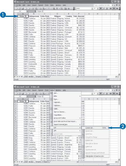
You can also choose the Create List command by pressing Ctrl+L.
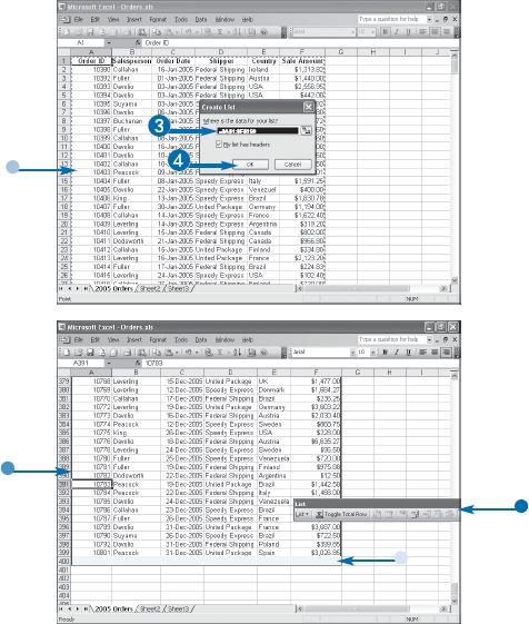
The Create List dialog box appears.
Excel selects the range that it will convert to a list.
Note
If you do not see the New Record item, click any cell within the list.
Extra
The New Record item is what makes lists so convenient for maintaining the source data for your PivotTable. To add a record to the list, click inside the list to display the New Record item, and then click the leftmost cell within the New Record row. Type your data for the first field and then press Tab to move to the second field. Excel displays a dialog box letting you know that you have inserted a row to your list; click OK. To avoid this dialog box in the future, select "Do not display this dialog again" (
After you have created a list, Excel offers a number of tools that enable you to easily maintain and work with the list. You will find these tools on the List toolbar, which you can display by clicking any cell within the list. For example, to add a record above the current record, click List→Insert→Row; to insert a new field in the list, click List→Insert→Column. You can also click List→Delete and then click either Row or Column to delete the current record or the current field. Finally, to convert the list back to a regular range, click List→Convert to Range.
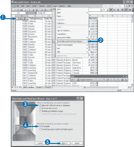
If the data you want to cross-tabulate exists as an Excel range or list, you can use the PivotTable and PivotChart Wizard to easily build a PivotTable report based on your data. The wizard takes you step by step through the process of choosing the type of report you want, specifying the location of your source data, and then choosing the location of the resulting PivotTable.
The PivotTable and PivotChart Wizard has three main steps. In the first step, you choose whether you want a PivotTable or a PivotChart. In this task, you learn how to build a PivotTable. If you want to learn how to build a PivotChart instead, see Chapter 9. The first wizard step also enables you to specify the type of data source you are using. In this task, you learn how to build a PivotTable based on data in an Excel list or range, which is the simplest and most common type of data source. To learn how to build PivotTables from other types of data sources, see Chapters 10 and 11.
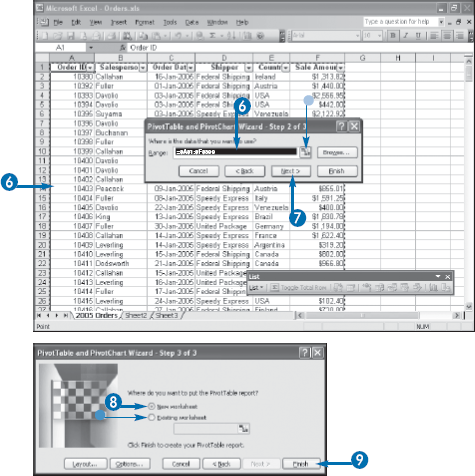
In the second step of the PivotTable and PivotChart Wizard, you specify the location of the list or range. If you choose a cell within the list or range in advance, the wizard automatically selects the surrounding list or range. Otherwise, you can click and drag with your mouse to select the data, or type the range address.
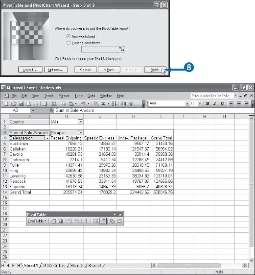
Finally, the third step of the wizard enables you to select a location for the new PivotTable report, and you can choose to place the PivotTable on either an existing worksheet or on a new worksheet.
The first PivotTable and PivotChart Wizard dialog box appears.
The second PivotTable and PivotChart Wizard dialog box appears.
The third PivotTable and PivotChart Wizard dialog box appears.
Note
To learn how to add fields directly from the wizard, see the task "Add Fields Using the PivotTable Wizard," later in this chapter
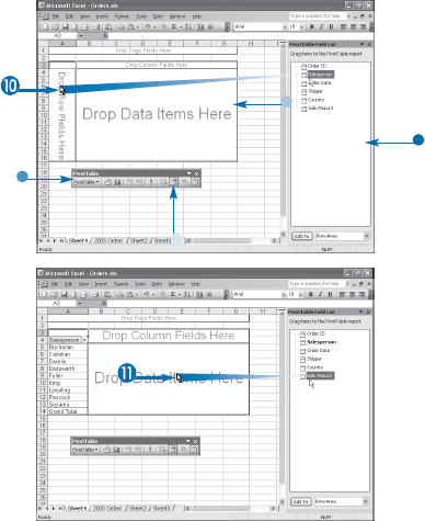
When you click Finish in the third PivotTable and PivotChart Wizard dialog box, Excel creates an empty PivotTable in a new worksheet or in the location you specified. The empty PivotTable displays four areas with the following labels: Drop Row Fields Here, Drop Column Fields Here, Drop Data Items Here, and Drop Page Fields Here. To complete the PivotTable, you must populate some or all of these areas with one or more fields from your data.
When you add a field to the row, column, or page area, Excel extracts the unique values from the field and displays them in the area. For example, if you add the Salesperson field to the row area, Excel displays the unique salesperson names as headings that run down the leftmost column of the PivotTable. Similarly, if you add the Shipper field to the column area, Excel displays the unique shipper names as headings that run across the top row of the PivotTable. Finally, if you add, say, the Country field to the page area, Excel displays the unique country names in a drop-down list above the PivotTable.
When you add a field to the data area, Excel performs calculations based on the numeric data in the field. The default calculation is sum, so if you add, for example, the Sale Amount field to the data area, Excel sums the Sale Amount values. How Excel calculates these sums depends on the fields you have added to the other areas. For example, if you add just the Salesperson field to the row area, Excel displays the sum of the Sale Amount values for each salesperson. You can also use other calculations such as Average and Count. See Chapter 8 to learn how to change the summary calculation.
Excel displays the field's unique values in the PivotTable's row area.
Excel displays the summary results in the PivotTable.

Excel displays the field's unique values in the PivotTable's column area.
Excel displays the field's unique values in the PivotTable's page drop-down list.
The basic PivotTable is complete.
Extra
If you are not comfortable dragging items with the mouse, you can also add fields to the PivotTable using the PivotTable Field List. To begin, use the PivotTable Field List to click the field you want to add to the PivotTable. In the drop-down list at the bottom of the PivotTable Field List, click
Do not attempt to edit the values that Excel displays in the row, column, or data areas. These values are generated or calculated automatically based on the data in the source range or list. You can edit these results, but doing so does not change the source data, and any changes you make will be overwritten the next time you refresh the PivotTable, as described in Chapter 3. If you want to change the value of a PivotTable cell, you must change the corresponding value or values in the source range and then refresh the PivotTable.
In the previous task, you learned how to use the PivotTable Field List to add fields directly to the PivotTable's row, data, column, and page areas. However, there may be times when you prefer not to use the PivotTable Field List. For example, if you already have the task pane displayed, then the combination of the PivotTable Field List and task pane could take up more than half the screen. In this case, you might prefer to close the PivotTable Field List so that you can see more of your worksheet — in the PivotTable toolbar, click the Toolbar Close button (
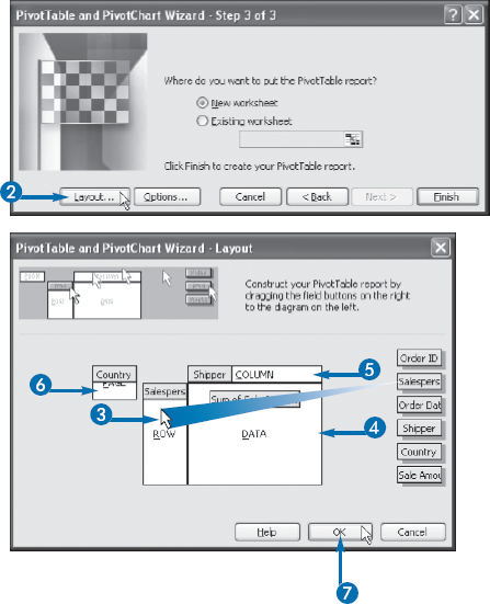
The PivotTable and PivotChart Wizard has a Layout dialog box that enables you to add fields from your list or range to the PivotTable's row, data, column, and page areas. The Layout dialog box is divided into two sections. On the right you see buttons for the various fields in your range or list; on the left, you see a diagram of the PivotTable showing four sections that represent the four areas: Row, Data, Column, and Page. For each area that you want to include in your PivotTable, you click and drag a field button and then drop it inside the appropriate area. When you close the Layout dialog box and finish the PivotTable and PivotChart Wizard, your PivotTable will be complete.
The source data that underlies a PivotTable rarely remains static. You, or someone else, may add or delete records, edit the existing data, or add or delete fields. Therefore, you will need to update your PivotTable from time to time to reflect these changes. In most cases, particularly when you are using an Excel list as the source data, you need only refresh the PivotTable to incorporate any changes to the original data. See Chapter 3 to learn how to refresh an existing PivotTable.
However, you may find that in certain cases, refreshing the PivotTable does not incorporate all the changes that have been made to the source data. Similarly, you may have an important meeting or presentation coming up and you want to make sure that your PivotTable is using the most up-to-date information. In both situations, you can ensure that your PivotTable uses the latest source data by re-creating the PivotTable. This involves running the PivotTable and PivotChart Wizard on the existing PivotTable and using the wizard to select the updated range or list.
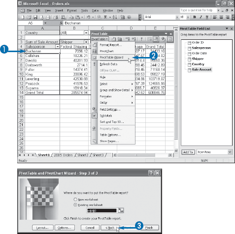
You can also right-click any cell in the PivotTable and then click PivotTable Wizard from the menu that appears.
The third PivotTable and PivotChart Wizard dialog box appears.
The second PivotTable and PivotChart Wizard dialog box appears.
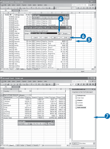
Excel re-creates the PivotTable.
If any fields were removed from the source data, Excel removes those fields from the PivotTable and from the PivotTable Field List.
If any fields were added to the source data, Excel adds those fields to the PivotTable Field List.