
102 3. ADVANCED INTEGRATION
-1
-1
3
3
R
(2,2)
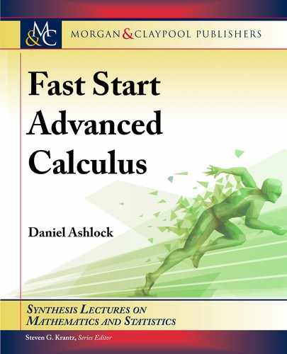
Figure 3.8: A non-rectangular region bounded by the x-axis, the line x D 2, and the line y D x.
Example 3.40 Find the volume underneath
f .x; y/ D 4 x
2
over the region bounded by
y D x
y D 2x
and
x D 2
Solution:
Start by drawing the region of integration.
is region has x bounds 0 x 2.
For a given value of x the region goes from the line y D x to the line y D 2x.

3.3. MULTIPLE INTEGRALS 103
-1
-1
5
3
is gives us sufficient information to set up the integral.
V D
Z
2
0
Z
2x
x
4 x
2
dy dx
D
Z
2
0
4y x
2
y
ˇ
ˇ
ˇ
ˇ
2x
x
dx
D
Z
2
0
8x 2x
3
4x Cx
3
dx
D
Z
2
0
4x x
3
dx
D 2x
2
1
4
x
4
ˇ
ˇ
ˇ
ˇ
2
0
D 8
1
4
16 0 C 0
D 4 units
3
˙

104 3. ADVANCED INTEGRATION
e regions we have used thus far have been based on functions that are easy to work with using
Cartesian coordinates.
To deal with other sorts of regions, we need to first develop a broader point of view.
-3
-3
3
3
R
Figure 3.9: Another sort of region – a disk of radius 2 centered at the origin.

3.3. MULTIPLE INTEGRALS 105
Knowledge Box 3.9
e differential of area
e change of area is
dA D dx dy D dy dx:
is permits us to change our integral notation to the following for the
integral of f .x; y/ over a region R
V D
Z Z
R
f .x; y/ dA:
In polar coordinates:
dA D r dr d:
Example 3.41 Find the area enclosed below the curve f .x; y/ D x
2
C y
2
over a disk of radius
2 centered at the origin.
Solution:
is volume is below the function f .x; y/ for points no farther from the origin than 2.
is means the region R is
x
2
C y
2
4:
In polar coordinates, this region is those points .r; / for which 0 r 2 and 0 2.
Since the polar/rectangular conversion equations tell us r
2
D x
2
C y
2
, f .r; / D r
2
.
Using polar coordinates the integral is:
V D
Z Z
R
f .r; / dA
D
Z
2
0
Z
2
0
r
2
r dr d

106 3. ADVANCED INTEGRATION
D
Z
2
0
Z
2
0
r
3
dr d
D
Z
2
0
1
4
r
4
ˇ
ˇ
ˇ
ˇ
2
0
d
D
Z
2
0
.
16=4 0
/
d
D
Z
2
0
4d
D 4
ˇ
ˇ
ˇ
ˇ
2
0
D 8 0 D 8 units
3
˙
e next example is a very important one for the theory of statistics. As you know if you have
studied statistics, the normal distribution has a probability distribution function of:
1
p
2
e
x
2
=2
e area under the curve of a probability distribution function must be equal to one. us,
if you have a function with an area greater than one, you must multiply it by a normalizing
constant equal to one over the area.
e following example shows where the normalizing constant
1
p
2
in the normal distri-
bution probability distribution function comes from.
e integral relies on a trick: squaring the integral and then shifting the squared integral to polar
coordinates. is changes an impossible integral into one that can be done without difficulty by
u-substitution. Sadly, this only permits the evaluation of the integral on the interval Œ1; 1;
the coordinate change is intractable except on the full interval where the function exists.
..................Content has been hidden....................
You can't read the all page of ebook, please click here login for view all page.