CHAPTER 4
UNDERSTANDING YIELD SPREADS
I. INTRODUCTION
The interest rate offered on a particular bond issue depends on the interest rate that can be earned on (1) risk-free instruments and (2) the perceived risks associated with the issue. We refer to the interest rates on risk-free instruments as the “level of interest rates.” The actions of a country’s central bank influence the level of interest rates as does the state of the country’s economy. In the United States, the level of interest rates depends on the state of the economy, the interest rate policies implemented by the Board of Governors of the Federal Reserve Board, and the government’s fiscal policies.
A casual examination of the financial press and dealer quote sheets shows a wide range of interest rates reported at any given point in time. Why are there differences in interest rates among debt instruments? We provided information on this topic in Chapters 1 and 2. In Chapter 1, we explained the various features of a bond while in Chapter 2 we explained how those features affect the risk characteristics of a bond relative to bonds without that feature.
In this chapter, we look more closely at the differences in yields offered by bonds in different sectors of the bond market and within a sector of the bond market. This information is used by investors in assessing the “relative value” of individual securities within a bond sector, or among sectors of the bond market. Relative value analysis is a process of ranking individual securities or sectors with respect to expected return potential. We will continue to use the terms “interest rate” and “yield” interchangeably.
II. INTEREST RATE DETERMINATION
Our focus in this chapter is on (1) the relationship between interest rates offered on different bond issues at a point in time and (2) the relationships among interest rates offered in different sectors of the economy at a given point in time. We will provide a brief discussion of the role of the U.S. Federal Reserve (the Fed), the policy making body whose interest rate policy tools directly influence short-term interest rates and indirectly influence long-term interest rates.
Once the Fed makes a policy decision it immediately announces the policy in a statement issued at the close of its meeting. The Fed also communicates its future intentions via public speeches or its Chairman’s testimony before Congress. Managers who pursue an active strategy of positioning a portfolio to take advantage of expected changes in interest rates watch closely the same key economic indicators that the Fed watches in order to anticipate a change in the Fed’s monetary policy and to assess the expected impact on short-term interest rates. The indicators that are closely watched by the Fed include non-farm payrolls, industrial production, housing starts, motor vehicle sales, durable good orders, National Association of Purchasing Management supplier deliveries, and commodity prices.
In implementing monetary policy, the Fed uses the following interest rate policy tools:
1. open market operations
2. the discount rate
3. bank reserve requirements
4. verbal persuasion to influence how bankers supply credit to businesses and consumers
Engaging in open market operations and changing the discount rate are the tools most often employed. Together, these tools can raise or lower the cost of funds in the economy. Open market operations do this through the Fed’s buying and selling of U.S. Treasury securities. This action either adds funds to the market (when Treasury securities are purchased) or withdraws funds from the market (when Treasury securities are sold). Fed open market operations influence the federal funds rate, the rate at which banks borrow and lend funds from each other. The discount rate is the interest rate at which banks can borrow on a collateralized basis at the Fed’s discount window. Increasing the discount rate makes the cost of funds more expensive for banks; the cost of funds is reduced when the discount rate is lowered. Changing bank reserve requirements is a less frequently used policy, as is the use of verbal persuasion to influence the supply of credit.
III. U.S. TREASURY RATES
The securities issued by the U.S. Department of the Treasury are backed by the full faith and credit of the U.S. government. Consequently, market participants throughout the world view these securities as being “default risk-free” securities. However, there are risks associated with owning U.S. Treasury securities.
The Treasury issues the following securities:
Treasury bills: Zero-coupon securities with a maturity at issuance of one year or less. The Treasury currently issues 1-month, 3-month, and 6-month bills.
Treasury notes: Coupon securities with maturity at issuance greater than 1 year but not greater than 10 years. The Treasury currently issues 2-year, 5-year, and 10-year notes.
Treasury bonds: Coupon securities with maturity at issuance greater than 10 years. Although Treasury bonds have traditionally been issued with maturities up to 30 years, the Treasury suspended issuance of the 30-year bond in October 2001.
Inflation-protection securities: Coupon securities whose principal’s reference rate is the Consumer Price Index.
The on-the-run issue or current issue is the most recently auctioned issue of Treasury notes and bonds of each maturity. The off-the-run issues are securities that were previously issued and are replaced by the on-the-run issue. Issues that have been replaced by several more recent issues are said to be “well off-the-run issues.”
The secondary market for Treasury securities is an over-the-counter market where a group of U.S. government securities dealers provides continuous bids and offers on specific outstanding Treasuries. This secondary market is the most liquid financial market in the world. Off-the-run issues are less liquid than on-the-run issues.
A. Risks of Treasury Securities
With this brief review of Treasury securities, let’s look at their risks. We listed the general risks in Chapter 2 and repeat them here: (1) interest rate risk, (2) call and prepayment risk, (3) yield curve risk, (4) reinvestment risk, (5) credit risk, (6) liquidity risk, (7) exchange-rate risk, (8) volatility risk, (9) inflation or purchasing power risk, and (10) event risk.
All fixed income securities, including Treasury securities, expose investors to interest rate risk.31 However, the degree of interest rate risk is not the same for all securities. The reason is that maturity and coupon rate affect how much the price changes when interest rates change. One measure of a security’s interest rate risk is its duration.32 Since Treasury securities, like other fixed income securities, have different durations, they have different exposures to interest rate risk as measured by duration.
Technically, yield curve risk and volatility risk are risks associated with Treasury securities. However, at this early stage of our understanding of fixed income analysis, we will not attempt to explain these risks. It is not necessary to understand these risks at this point in order to appreciate the material that follows in this section.
Because Treasury securities are noncallable, there is no reinvestment risk due to an issue being called.33 Treasury coupon securities carry reinvestment risk because in order to realize the yield offered on the security, the investor must reinvest the coupon payments received at an interest rate equal to the computed yield. So, all Treasury coupon securities are exposed to reinvestment risk. Treasury bills are not exposed to reinvestment risk because they are zero-coupon instruments.
As for credit risk, the perception in the global financial community is that Treasury securities have no credit risk. In fact, when market participants and the popular press state that Treasury securities are “risk free,” they are referring to credit risk.
Treasury securities are highly liquid. However, on-the-run and off-the-run Treasury securities trade with different degrees of liquidity. Consequently, the yields offered by on-the-run and off-the-run issues reflect different degrees of liquidity.
Since U.S. Treasury securities are dollar denominated, there is no exchange-rate risk for an investor whose domestic currency is the U.S. dollar. However, non-U.S. investors whose domestic currency is not the U.S. dollar are exposed to exchange-rate risk.
Fixed-rate Treasury securities are exposed to inflation risk. Treasury inflation protection securities (TIPS) have a coupon rate that is effectively adjusted for the rate of inflation and therefore have protection against inflation risk.
EXHIBIT 1 Relationship Between Yield and Maturity for On-the-Run Treasury Issues on February 8, 2002
Source: Global Relative Value, Lehman Brothers, Fixed Income Research, February 11, 2002, p. 128.
| Issue (maturity) | Yield (%) |
|---|---|
| 1 month | 1.68 |
| 3 months | 1.71 |
| 6 months | 1.81 |
| 1 year1 | 2.09 |
| 2 years | 2.91 |
| 5 years | 4.18 |
| 10 years | 4.88 |
| 30 years2 | 5.38 |
| 1 The 1-year issue is based on the 2-year issue closest to maturing in one year. | |
| 2The 30-year issue shown is based on the last 30-year issue before the Treasury suspended issuance of Treasury bonds in October 2001. | |
Finally, the yield on Treasury securities is impacted by a myriad of events that can be classified as political risk, a form of event risk. The actions of monetary and fiscal policy in the United States, as well as the actions of other central banks and governments, can have an adverse or favorable impact on U.S. Treasury yields.
B. The Treasury Yield Curve
Given that Treasury securities do not expose investors to credit risk, market participants look at the yield offered on an on-the-run Treasury security as the minimum interest rate required on a non-Treasury security with the same maturity. The relationship between yield and maturity of on-the-run Treasury securities on February 8, 2002 is displayed in Exhibit 1 in tabular form. The relationship shown in Exhibit 1 is called the Treasury yield curve—even though the “curve” shown in the exhibit is presented in tabular form.
The information presented in Exhibit 1 indicates that the longer the maturity the higher the yield and is referred to as an upward sloping yield curve. Since this is the most typical shape for the Treasury yield curve, it is also referred to as a normal yield curve. Other relationships have been observed. An inverted yield curve indicates that the longer the maturity, the lower the yield. For a flat yield curve the yield is approximately the same regardless of maturity.
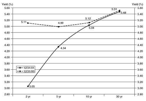
Exhibit 2 provides a graphic example of the variants of these shapes and also shows how a yield curve can change over time. In the exhibit, the yield curve at the beginning of 2001 was inverted up to the 5-year maturity but was upward sloping beyond the 5-year maturity. By December 2001, all interest rates had declined. As seen in the exhibit, interest rates less than the 10-year maturity dropped substantially more than longer-term rates resulting in an upward sloping yield curve.
The number of on-the-run securities available in constructing the yield curve has decreased over the last two decades. While the 1-year and 30-year yields are shown in the February 8, 2002 yield curve, as of this writing there is no 1-year Treasury bill and the maturity of the 30-year Treasury bond (the last one issued before suspension of the issuance of 30-year Treasury bonds) will decline over time. To get a yield for maturities where no on-the-run Treasury issue exists, it is necessary to interpolate from the yield of two on-the-run issues. Several methodologies are used in practice. (The simplest is just a linear interpolation.) Thus, when market participants talk about a yield on the Treasury yield curve that is not one of the available on-the-run maturities—for example, the 8-year yield—it is only an approximation.
EXHIBIT 2 U.S. Treasury Yield Curve: December 2000 and December 2001
Source: Lehman Brothers Fixed Income Research, Global Fixed Income Strategy “Playbook,” January 2002.
It is critical to understand that any non-Treasury issue must offer a premium above the yield offered for the same maturity on-the-run Treasury issue. For example, if a corporation wanted to offer a 10-year noncallable issue on February 8, 2002, the issuer must offer a yield greater than 4.88% (the yield for the 10-year on-the-run Treasury issue). How much greater depends on the additional risks associated with investing in the 10-year corporate issue compared to investors in the 10-year on-the-run Treasury issue. Even off-the-run Treasury issues must offer a premium to reflect differences in liquidity.
Two factors complicate the relationship between maturity and yield as portrayed by the yield curve. The first is that the yield for on-the-run issues may be distorted by the fact that purchase of these securities can be financed at lower rates and as a result these issues offer artificially low yields. To clarify, some investors purchase securities with borrowed funds and use the securities purchased as collateral for the loan. This type of collateralized borrowing is called a repurchase agreement. Since dealers want to obtain use of these securities for their own trading activities, they are willing to lend funds to investors at a lower interest rate than is otherwise available for borrowing in the market. Consequently, incorporated into the price of an on-the-run Treasury security is the cheaper financing available, resulting in a lower yield for an on-the-run issue than would prevail in the absence of this financing advantage.
The second factor complicating the comparison of on-the-run and off-the-run Treasury issues (in addition to liquidity differences) is that they have different interest rate risks and different reinvestment risks. So, for example, if the coupon rate for the 5-year on-the-run Treasury issue in February 2002 is 4.18% and an off-the-run Treasury issue with just less than 5 years to maturity has a 5.25% coupon rate, the two bonds have different degrees of interest rate risk. Specifically, the on-the-run issue has greater interest rate risk (duration) because of the lower coupon rate. However, it has less reinvestment risk because the coupon rate is lower.
Because of this, when market participants talk about interest rates in the Treasury market and use these interest rates to value securities they look at another relationship in the Treasury market: the relationship between yield and maturity for zero-coupon Treasury securities. But wait, we said that the Treasury only issues three zero-coupon securities—1-month, 3-month, and 6-month Treasury bills. Where do we obtain the relationship between yield and maturity for zero-coupon Treasury securities? We discuss this next.
1. Theories of the Term Structure of Interest Rates What information does the yield curve reveal? How can we explain and interpret changes in the yield curve? These questions are of great interest to anyone concerned with such tasks as the valuation of multiperiod securities, economic forecasting, and risk management. Theories of the term structure of interest rates34 address these questions. Here we introduce the three main theories or explanations of the term structure. We shall present these theories intuitively.35
The three main term structure theories are:
• the pure expectations theory (unbiased expectations theory)
• the liquidity preference theory (or liquidity premium theory)
• the market segmentation theory
Each theory is explained below.
a. Pure Expectations Theory The pure expectations theory makes the simplest and most direct link between the yield curve and investors’ expectations about future interest rates, and, because long-term interest rates are plausibly linked to investor expectations about future inflation, it also opens the door to some interesting economic interpretations.
The pure expectations theory explains the term structure in terms of expected future short-term interest rates. According to the pure expectations theory, the market sets the yield on a two-year bond so that the return on the two-year bond is approximately equal to the return on a one-year bond plus the expected return on a one-year bond purchased one year from today.
Under this theory, a rising term structure indicates that the market expects short-term rates to rise in the future. For example, if the yield on the two-year bond is higher than the yield on the one-year bond, according to this theory, investors expect the one-year rate a year from now to be sufficiently higher than the one-year rate available now so that the two ways of investing for two years have the same expected return. Similarly, a flat term structure reflects an expectation that future short-term rates will be unchanged from today’s short-term rates, while a falling term structure reflects an expectation that future short-term rates will decline. This is summarized below:
The implications above are the broadest interpretation of the theory.
How does the pure expectations theory explain a humped yield curve? According to the theory, this can result when investors expect the returns on one-year securities to rise for a number of years, then fall for a number of years.
The relationships that the table above illustrates suggest that the shape of the yield curve contains information regarding investors’ expectations about future inflation. A pioneer of the theory of interest rates (the economist Irving Fisher) asserted that interest rates reflect the sum of a relatively stable real rate of interest plus a premium for expected inflation. Under this hypothesis, if short-term rates are expected to rise, investors expect inflation to rise as well. An upward (downward) sloping term structure would mean that investors expected rising (declining) future inflation. Much economic discussion in the financial press and elsewhere is based on this interpretation of the yield curve.
The shortcoming of the pure expectations theory is that it assumes investors are indifferent to interest rate risk and any other risk factors associated with investing in bonds with different maturities.
| Shape of term structure | Implication according to pure expectations theory |
|---|---|
| upward sloping (normal) | rates expected to rise |
| downward sloping (inverted) | rates expected to decline |
| flat | rates not expected to change |
b. Liquidity Preference Theory The liquidity preference theory asserts that market participants want to be compensated for the interest rate risk associated with holding longer-term bonds. The longer the maturity, the greater the price volatility when interest rates change and investors want to be compensated for this risk. According to the liquidity preference theory, the term structure of interest rates is determined by (1) expectations about future interest rates and (2) a yield premium for interest rate risk.36 Because interest rate risk increases with maturity, the liquidity preference theory asserts that the yield premium increases with maturity.
Consequently, based on this theory, an upward-sloping yield curve may reflect expectations that future interest rates either (1) will rise, or (2) will be unchanged or even fall, but with a yield premium increasing with maturity fast enough to produce an upward sloping yield curve. Thus, for an upward sloping yield curve (the most frequently observed type), the liquidity preference theory by itself has nothing to say about expected future short-term interest rates. For flat or downward sloping yield curves, the liquidity preference theory is consistent with a forecast of declining future short-term interest rates, given the theory’s prediction that the yield premium for interest rate risk increases with maturity.
Because the liquidity preference theory argues that the term structure is determined by both expectations regarding future interest rates and a yield premium for interest rate risk, it is referred to as biased expectations theory.
c. Market Segmentation Theory Proponents of the market segmentation theory argue that within the different maturity sectors of the yield curve the supply and demand for funds determine the interest rate for that sector. That is, each maturity sector is an independent or segmented market for purposes of determining the interest rate in that maturity sector. Thus, positive sloping, inverted, and humped yield curves are all possible. In fact, the market segmentation theory can be used to explain any shape that one might observe for the yield curve.
Let’s understand why proponents of this theory view each maturity sector as independent or segmented. In the bond market, investors can be divided into two groups based on their return needs: investors that manage funds versus a broad-based bond market index and those that manage funds versus their liabilities. The easiest case is for those that manage funds against liabilities. Investors managing funds where liabilities represent the benchmark will restrict their activities to the maturity sector that provides the best match with the maturity of their liabilities.37 This is the basic principle of asset-liability management. If these investors invest funds outside of the maturity sector that provides the best match against liabilities, they are exposing themselves to the risks associated with an asset-liability mismatch. For example, consider the manager of a defined benefit pension fund. Since the liabilities of a defined benefit pension fund are long-term, the manager will invest in the long-term maturity sector of the bond market. Similarly, commercial banks whose liabilities are typically short-term focus on short-term fixed-income investments. Even if the rate on long-term bonds were considerably more attractive than that on short-term investments, according to the market segmentation theory commercial banks will restrict their activities to investments at the short end of the yield curve. Reinforcing this notion of a segmented market are restrictions imposed on financial institutions that prevent them from mismatching the maturity of assets and liabilities.
A variant of the market segmentation theory is the preferred habitat theory. This theory argues that investors prefer to invest in particular maturity sectors as dedicated by the nature of their liabilities. However, proponents of this theory do not assert that investors would be unwilling to shift out of their preferred maturity sector; instead, it is argued that if investors are given an inducement to do so in the form of a yield premium they will shift out of their preferred habitat. The implication of the preferred habitat theory for the shape of the yield curve is that any shape is possible.
C. Treasury Strips
Although the U.S. Department of the Treasury does not issue zero-coupon Treasury securities with maturity greater than one year, government dealers can synthetically create zero-coupon securities, which are effectively guaranteed by the full faith and credit of the U.S. government, with longer maturities. They create these securities by separating the coupon payments and the principal payment of a coupon-bearing Treasury security and selling them off separately. The process, referred to as stripping a Treasury security, results in securities called Treasury strips. The Treasury strips created from coupon payments are called Treasury coupon strips and those created from the principal payment are called Treasury principal strips. We explained the process of creating Treasury strips in Chapter 3.
Because zero-coupon instruments have no reinvestment risk, Treasury strips for different maturities provide a superior relationship between yield and maturity than do securities on the on-the-run Treasury yield curve. The lack of reinvestment risk eliminates the bias resulting from the difference in reinvestment risk for the securities being compared. Another advantage is that the duration of a zero-coupon security is approximately equal to its maturity. Consequently, when comparing bond issues against Treasury strips, we can compare them on the basis of duration.
The yield on a zero-coupon security has a special name: the spot rate. In the case of a Treasury security, the yield is called a Treasury spot rate. The relationship between maturity and Treasury spot rates is called the term structure of interest rates. Sometimes discussions of the term structure of interest rates in the Treasury market get confusing. The Treasury yield curve and the Treasury term structure of interest rates are often used interchangeably. While there is a technical difference between the two, the context in which these terms are used should be understood.
IV. YIELDS ON NON-TREASURY SECURITIES
Despite the imperfections of the Treasury yield curve as a benchmark for the minimum interest rate that an investor requires for investing in a non-Treasury security, it is commonplace to refer to the additional yield over the benchmark Treasury issue of the same maturity as the yield spread. In fact, because non-Treasury sectors of the fixed income market offer a yield spread to Treasury securities, non-Treasury sectors are commonly referred to as spread sectors and non-Treasury securities in these sectors are referred to as spread products.
A. Measuring Yield Spreads
While it is common to talk about spreads relative to a Treasury security of the same maturity, a yield spread between any two bond issues can be easily computed. In general, the yield spread between any two bond issues, bond X and bond Y, is computed as follows:
where bond Y is considered the reference bond (or benchmark) against which bond X is measured.
yield spread = yield on bond X − yield on bond Y
When a yield spread is computed in this manner it is referred to as an absolute yield spread and it is measured in basis points. For example, on February 8, 2002, the yield on the 10-year on-the-run Treasury issue was 4.88% and the yield on a single A rated 10-year industrial bond was 6.24%. If bond X is the 10-year industrial bond and bond Y is the 10-year on-the-run Treasury issue, the absolute yield spread was:
yield spread = 6.24% − 4.88% = 1.36% or 136 basis points
Unless otherwise specified, yield spreads are typically measured in this way. Yield spreads can also be measured on a relative basis by taking the ratio of the yield spread to the yield of the reference bond. This is called a relative yield spread and is computed as shown below, assuming that the reference bond is bond Y:

Sometimes bonds are compared in terms of a yield ratio, the quotient of two bond yields, as shown below:

Typically, in the U.S. bond market when these measures are computed, bond Y (the reference bond) is a Treasury issue. In that case, the equations for the yield spread measures are as follows:

For the above example comparing the yields on the 10-year single A rated industrial bond and the 10-year on-the-run Treasury, the relative yield spread and yield ratio are computed below:

The reason for computing yield spreads in terms of a relative yield spread or a yield ratio is that the magnitude of the yield spread is affected by the level of interest rates. For example, in 1957 the yield on Treasuries was about 3%. At that time, the absolute yield spread between triple B rated utility bonds and Treasuries was 40 basis points. This was a relative yield spread of 13% (0.40% divided by 3%). However, when the yield on Treasuries exceeded 10% in 1985, an absolute yield spread of 40 basis points would have meant a relative yield spread of only 4% (0.40% divided by 10%). Consequently, in 1985 an absolute yield spread greater than 40 basis points would have been required in order to produce a similar relative yield spread.
In this chapter, we will focus on the yield spread as most commonly measured, the absolute yield spread. So, when we refer to yield spread, we mean absolute yield spread.
Whether we measure the yield spread as an absolute yield spread, a relative yield spread, or a yield ratio, the question to answer is what causes the yield spread between two bond issues. Basically, active bond portfolio strategies involve assessing the factors that cause the yield spread, forecasting how that yield spread may change over an investment horizon, and taking a position to capitalize on that forecast.
B. Intermarket Sector Spreads and Intramarket Spreads
The bond market is classified into sectors based on the type of issuer. In the United States, these sectors include the U.S. government sector, the U.S. government agencies sector, the municipal sector, the corporate sector, the mortgage-backed securities sector, the asset-backed securities sector, and the foreign (sovereign, supranational, and corporate) sector. Different sectors are generally perceived as offering different risks and rewards.
The major market sectors are further divided into sub-sectors reflecting common economic characteristics. For example, within the corporate sector, the subsectors are: (1) industrial companies, (2) utility companies, (3) finance companies, and (4) banks. In the market for asset-backed securities, the sub-sectors are based on the type of collateral backing the security. The major types are securities backed by pools of (1) credit card receivables, (2) home equity loans, (3) automobile loans, (4) manufactured housing loans, and (5) student loans. Excluding the Treasury market sector, the other market sectors have a wide range of issuers, each with different abilities to satisfy their contractual obligations. Therefore, a key feature of a debt obligation is the nature of the issuer.
The yield spread between the yields offered in two sectors of the bond market with the same maturity is referred to as an intermarket sector spread. The most common intermarket sector spread calculated by market participants is the yield spread between a non-Treasury sector and Treasury securities with the same maturity.
The yield spread between two issues within a market sector is called an intramarket sector spread. As with Treasury securities, a yield curve can be estimated for a given issuer. The yield spread typically increases with maturity. The yield spreads for a given issuer can be added to the yield for the corresponding maturity of the on-the-run Treasury issue. The resulting yield curve is then an issuer’s on-the-run yield curve.
The factors other than maturity that affect the intermarket and intramarket yield spreads are (1) the relative credit risk of the two issues, (2) the presence of embedded options, (3) the liquidity of the two issues, and (4) the taxability of interest received by investors.
C. Credit Spreads
The yield spread between non-Treasury securities and Treasury securities that are identical in all respects except for credit rating is referred to as a credit spread or quality spread. “Identical in all respects except credit rating” means that the maturities are the same and that there are no embedded options.
For example, Exhibit 3 shows information on the yield spread within the corporate sector by credit rating and maturity, for the 90-day period ending February 8, 2002. The high, low, and average spreads for the 90-day period are reported. Note that the lower the credit rating, the higher the credit spread. Also note that, for a given sector of the corporate market and a given credit rating, the credit spread increases with maturity.
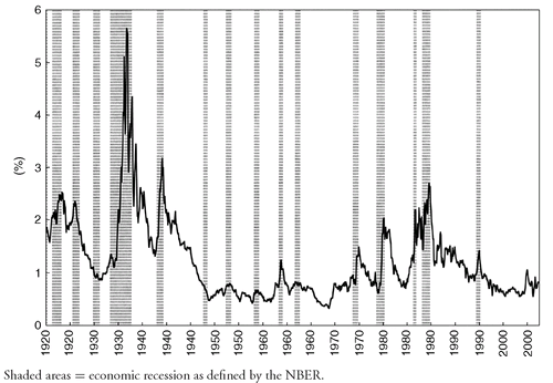
It is argued that credit spreads between corporates and Treasuries change systematically with changes in the economy. Credit spreads widen (i.e., become larger) in a declining or contracting economy and narrow (i.e., become smaller) during economic expansion. The economic rationale is that, in a declining or contracting economy, corporations experience declines in revenue and cash flow, making it more difficult for corporate issuers to service their contractual debt obligations. To induce investors to hold spread products as credit quality deteriorates, the credit spread widens. The widening occurs as investors sell off corporates and invest the proceeds in Treasury securities (popularly referred to as a “flight to quality”). The converse is that, during economic expansion and brisk economic activity, revenue and cash flow increase, increasing the likelihood that corporate issuers will have the capacity to service their contractual debt obligations.
Exhibit 4 provides evidence of the impact of the business cycle on credit spreads since 1919. The credit spread in the exhibit is the difference between Baa rated and Aaa rated corporate bonds; the shaded areas in the exhibit represent periods of economic recession as defined by the National Bureau of Economic Research (NBER). In general, corporate credit spreads tightened during the early stages of economic expansion, and spreads widened sharply during economic recessions. In fact, spreads typically begin to widen before the official beginning of an economic recession.38
EXHIBIT 3 Credit Spreads (in Basis Points) in the Corporate Sector on February 8, 2002
Source: Abstracted from Global Relative Value, Lehman Brothers, Fixed Income Research, February 11, 2002, p. 133.
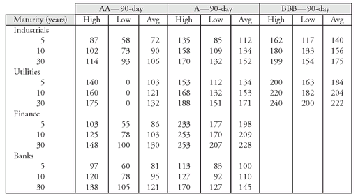
EXHIBIT 4 Credit Spreads Between Baa and Aaa Corporate Bonds Over the Business Cycle Since 1919
Source: Exhibit 1 in Leland E. Crabbe and Frank J. Fabozzi, Managing a Corporate Portfolio (Hoboken, NJ: John Wiley & Sons, 2002), p. 154.
Some market observers use the yield spread between issuers in cyclical and non-cyclical industry sectors as a proxy for yield spreads due to expected economic conditions. The rationale is as follows. While companies in both cyclical and non-cyclical industries are adversely affected by expectations of a recession, the impact is greater for cyclical industries. As a result, the yield spread between issuers in cyclical and non-cyclical industry sectors will widen with expectations of a contracting economy.
D. Including Embedded Options
It is not uncommon for a bond issue to include a provision that gives either the issuer and/or the bondholder an option to take some action against the other party. The most common type of option in a bond issue is the call provision that grants the issuer the right to retire the debt, fully or partially, before the scheduled maturity date.
The presence of an embedded option has an effect on both the yield spread of an issue relative to a Treasury security and the yield spread relative to otherwise comparable issues that do not have an embedded option. In general, investors require a larger yield spread to a comparable Treasury security for an issue with an embedded option that is favorable to the issuer (e.g. a call option) than for an issue without such an option. In contrast, market participants require a smaller yield spread to a comparable Treasury security for an issue with an embedded option that is favorable to the investor (e.g., put option or conversion option). In fact, for a bond with an option favorable to an investor, the interest rate may be less than that on a comparable Treasury security.
Even for callable bonds, the yield spread depends on the type of call feature. For a callable bond with a deferred call, the longer the deferred call period, the greater the call protection provided to the investor. Thus, all other factors equal, the longer the deferred call period, the lower the yield spread attributable to the call feature.
A major part of the bond market is the mortgage-backed securities sector.39 These securities expose an investor to prepayment risk and the yield spread between a mortgage-backed security and a comparable Treasury security reflects this prepayment risk. To see this, consider a basic mortgage-backed security called a Ginnie Mae passthrough security. This security is backed by the full faith and credit of the U.S. government. Consequently, the yield spread between a Ginnie Mae passthrough security and a comparable Treasury security is not due to credit risk. Rather, it is primarily due to prepayment risk. For example, Exhibit 5 reports the yield on 30-year Ginnie Mae passthrough securities with different coupon rates. The first issue to be addressed is the maturity of the comparable Treasury issue against which the Ginnie Mae should be benchmarked in order to calculate a yield spread. This is an issue because a mortgage passthrough security is an amortizing security that repays principal over time rather than just at the stated maturity date (30 years in our illustration). Consequently, while the stated maturity of a Ginnie Mae passthrough is 30 years, its yield should not be compared to the yield on a 30-year Treasury issue. For now, you can see that the Treasury benchmark in Exhibit 5 depends on the coupon rate. The yield spread, shown in the second column, depends on the coupon rate.
EXHIBIT 5 Yield Spreads and Option-Adjusted Spread (OAS) for Ginnie Mae 30-Year Passthrough Securities (February 8, 2002)
Source: Abstracted from Global Relative Value, Lehman Brothers, Fixed Income Research, February 11, 2002, p. 132.

In general, when a yield spread is cited for an issue that is callable, part of the spread reflects the risk associated with the embedded option. Reported yield spreads do not adjust for embedded options. The raw yield spreads are sometimes referred to as nominal spreads—nominal in the sense that the value of embedded options has not been removed in computing an adjusted yield spread. The yield spread that adjusts for the embedded option is OAS.
The last four columns in Exhibit 5 show Lehman Brothers’ estimate of the option-adjusted spread for the 30-year Ginnie Mae passthroughs shown in the exhibit—the option-adjusted spread on February 8, 2002 and for the prior 90-day period (high, low, and average). The nominal spread is the yield spread shown in the second column. Notice that the option-adjusted spread is considerably less than the nominal spread. For example, for the 7.5% coupon issue the nominal spread is 155 basis points. After adjusting for the prepayment risk (i.e., the embedded option), the spread as measured by the option-adjusted spread is considerably less, 63 basis points.
E. Liquidity
Even within the Treasury market, a yield spread exists between off-the-run Treasury issues and on-the-run Treasury issues of similar maturity due to differences in liquidity and the effects of the repo market. Similarly, in the spread sectors, generic on-the-run yield curves can be estimated and the liquidity spread due to an off-the-run issue can be computed.
A Lehman Brother’s study found that one factor that affects liquidity (and therefore the yield spread) is the size of an issue—the larger the issue, the greater the liquidity relative to a smaller issue, and the greater the liquidity, the lower the yield spread.40
F. Taxability of Interest Income
In the United States, unless exempted under the federal income tax code, interest income is taxable at the federal income tax level. In addition to federal income taxes, state and local taxes may apply to interest income.
EXHIBIT 6 Yield Ratio for AAA General Obligation Municipal Bonds to U.S. Treasuries of the Same Maturity (February 12, 2002)
Source: Bloomberg Financial Markets.
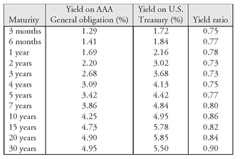
The federal tax code specifically exempts interest income from qualified municipal bond issues from taxation.41 Because of the tax-exempt feature of these municipal bonds, the yield on municipal bonds is less than that on Treasuries with the same maturity. Exhibit 6 shows this relationship on February 12, 2002, as reported by Bloomberg Financial Markets. The yield ratio shown for municipal bonds is the ratio of AAA general obligation bond yields to yields for the same maturity on-the-run Treasury issue. 42
The difference in yield between tax-exempt securities and Treasury securities is typically measured not in terms of the absolute yield spread but as a yield ratio. More specifically, it is measured as the quotient of the yield on a tax-exempt security relative to the yield on a comparable Treasury security. This is reported in Exhibit 6. The yield ratio has changed over time due to changes in tax rates, as well as other factors. The higher the tax rate, the more attractive the tax-exempt feature and the lower the yield ratio.
The U.S. municipal bond market is divided into two bond sectors: general obligation bonds and revenue bonds. For the tax-exempt bond market, the benchmark for calculating yield spreads is not Treasury securities, but rather a generic AAA general obligation yield curve constructed by dealer firms active in the municipal bond market and by data/analytics vendors.
1. After-Tax Yield and Taxable-Equivalent Yield The yield on a taxable bond issue after federal income taxes are paid is called the after-tax yield and is computed as follows:
after-tax yield = pre-tax yield × (1 − marginal tax rate)
Of course, the marginal tax rate 43 varies among investors. For example, suppose a taxable bond issue offers a yield of 5% and is acquired by an investor facing a marginal tax rate of 31%. The after-tax yield would then be:
after-tax yield = 0.05 × (1 − 0.31) = 0.0345 = 3.45%
Alternatively, we can determine the yield that must be offered on a taxable bond issue to give the same after-tax yield as a tax-exempt issue. This yield is called the taxable-equivalent yield or tax-equivalent yield and is computed as follows:

For example, consider an investor facing a 31% marginal tax rate who purchases a tax-exempt issue with a yield of 4%. The taxable-equivalent yield is then:
Notice that the higher the marginal tax rate, the higher the taxable equivalent yield. For instance, in our last example if the marginal tax rate is 40% rather than 31%, the taxable-equivalent yield would be 6.67% rather than 5.80%, as shown below:
Some state and local governments tax interest income from bond issues that are exempt from federal income taxes. Some municipalities exempt interest income from all municipal issues from taxation, while others do not. Some states exempt interest income from bonds issued by municipalities within the state but tax the interest income from bonds issued by municipalities outside of the state. The implication is that two municipal securities with the same credit rating and the same maturity may trade at different yield spreads because of the relative demand for bonds of municipalities in different states. For example, in a high income tax state such as New York, the demand for bonds of New York municipalities drives down their yields relative to bonds issued by municipalities in a zero income tax state such as Texas.
G. Technical Factors
At times, deviations from typical yield spreads are caused by temporary imbalances between supply and demand. For example, in the second quarter of 1999, issuers became concerned that the Fed would pursue a policy to increase interest rates. In response, a record issuance of corporate securities resulted in an increase in the yield spread between corporates and Treasuries.
In the municipal market, yield spreads are affected by the temporary oversupply of issues within a market sector. For example, a substantial new issue volume of high-grade state general obligation bonds may tend to decrease the yield spread between high-grade and low-grade revenue bonds. In a weak market environment, it is easier for high-grade municipal bonds to come to market than for weaker credits. So at times high grades flood weak markets even when there is a relative scarcity of medium- and low-grade municipal bond issues.
Since technical factors cause temporary misalignments of the yield spread relationship, some investors look at the forward calendar of planned offerings to project the impact on future yield spreads. Some corporate analysts identify the risk of yield spread changes due to the supply of new issues when evaluating issuers or sectors.
V. NON-U.S. INTEREST RATES
The same factors that affect yield spreads in the United States are responsible for yield spreads in other countries and between countries. Major non-U.S. bond markets have a government benchmark yield curve similar to that of the U.S. Treasury yield curve. Exhibit 7 shows the government yield curve as of the beginning and end of 2001 for Germany, Japan, the U.K., and France. These yield curves are presented to illustrate the different shapes and the way in which they can change. Notice that only the Japanese yield curve shifted in an almost parallel fashion (i.e., the rate for all maturities changed by approximately the same number of basis points).
EXHIBIT 7 Yield Curves in Germany, Japan, the U.K., and France: 2001
Source: Lehman Brothers Fixed Income Research, Global Fixed Income Strategy “Playbook,” January 2002.
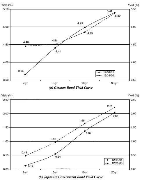
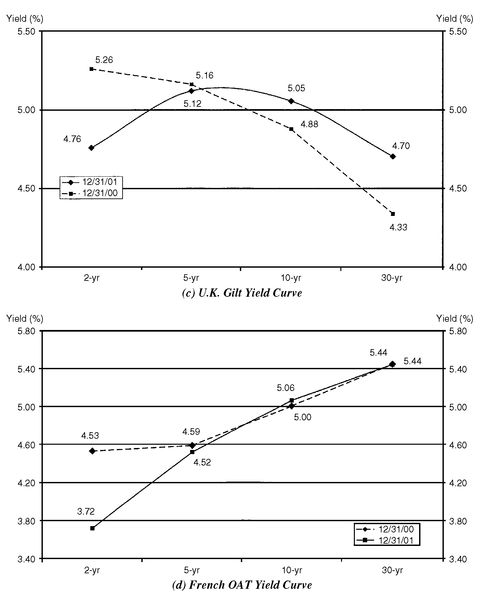
The German bond market is the largest market for publicly issued bonds in Europe. The yields on German government bonds are viewed as benchmark interest rates in Europe. Because of the important role of the German bond market, nominal spreads are typically computed relative to German government bonds (German bunds).
Institutional investors who borrow funds on a short-term basis to invest (referred to as “funded investors”) obviously desire to earn an amount in excess of their borrowing cost. The most popular borrowing cost reference rate is the London interbank offered rate (LIBOR). LIBOR is the interest rate at which banks pay to borrow funds from other banks in the London interbank market. The borrowing occurs via a cash deposit of one bank (the lender) into a certificate of deposit (CD) in another bank (the borrower). The maturity of the CD can be from overnight to five years. So, 3-month LIBOR represents the interest rate paid on a CD that matures in three months. The CD can be denominated in one of several currencies. The currencies for which LIBOR is reported are the U.S. dollar, the British pound, the Euro, the Canadian dollar, the Australian dollar, the Japanese yen, and Swiss francs. When it is denominated in U.S. dollars, it is referred to as a Eurodollar CD. LIBOR is determined for every London business day by the British Bank Association (BBA) by maturity and for each currency and is reported by various services.
Entities seeking to borrow funds pays a spread over LIBOR and seek to earn a spread over that funding cost when they invest the borrowed funds. So, for example, if the 3-month borrowing cost for a funded investor is 3-month LIBOR plus 25 basis points and the investor can earn 3-month LIBOR plus 125 basis points for three months, then the investor earns a spread of 100 basis points for three months (125 basis points-25 basis points).
VI. SWAP SPREADS
Another important spread measure is the swap spread.
A. Interest Rate Swap and the Swap Spread
In an interest rate swap, two parties (called counterparties) agree to exchange periodic interest payments. The dollar amount of the interest payments exchanged is based on a predetermined dollar principal, which is called the notional principal or notional amount. The dollar amount each counterparty pays to the other is the agreed-upon periodic interest rate times the notional principal. The only dollars exchanged between the parties are the interest payments, not the notional principal. In the most common type of swap, one party agrees to pay the other party fixed interest payments at designated dates for the life of the swap. This party is referred to as the fixed-rate payer. The fixed rate that the fixed-rate payer pays is called the swap rate. The other party, who agrees to make interest rate payments that float with some reference rate, is referred to as the fixed-rate receiver.
The reference rates used for the floating rate in an interest rate swap is one of various money market instruments: LIBOR (the most common reference rate used in swaps), Treasury bill rate, commercial paper rate, bankers’ acceptance rate, federal funds rate, and prime rate.
The convention that has evolved for quoting a swap rate is that a dealer sets the floating rate equal to the reference rate and then quotes the fixed rate that will apply. The fixed rate has a specified “spread” above the yield for a Treasury with the same term to maturity as the swap. This specified spread is called the swap spread. The swap rate is the sum of the yield for a Treasury with the same maturity as the swap plus the swap spread.
To illustrate an interest rate swap in which one party pays fixed and receives floating, assume the following:
term of swap: 5 years
swap spread: 50 basis points
reference rate: 3-month LIBOR
notional amount: $50 million
frequency of payments: every three months
swap spread: 50 basis points
reference rate: 3-month LIBOR
notional amount: $50 million
frequency of payments: every three months
Suppose also that the 5-year Treasury rate is 5.5% at the time the swap is entered into. Then the swap rate will be 6%, found by adding the swap spread of 50 basis points to the 5-year Treasury yield of 5.5%.
This means that the fixed-rate payer agrees to pay a 6% annual rate for the next five years with payments made quarterly and receive from the fixed-rate receiver 3-month LIBOR with the payments made quarterly. Since the notional amount is $50 million, this means that every three months, the fixed-rate payer pays $750,000 (6% times $50 million divided by 4). The fixed-rate receiver pays 3-month LIBOR times $50 million divided by 4. The table below shows the payment made by the fixed-rate receiver to the fixed-rate payer for different values of 3-month LIBOR:44
| If 3-month LIBOR is | Annual dollar amount | Quarterly payment |
|---|---|---|
| 4% | $2,000,000 | $500,000 |
| 5% | 2,500,000 | 625,000 |
| 6% | 3,000,000 | 750,000 |
| 7% | 3,500,000 | 875,000 |
| 8% | 4,000,000 | 1,000,000 |
In practice, the payments are netted out. For example, if 3-month LIBOR is 4%, the fixed-rate receiver would receive $750,000 and pay to the fixed-rate payer $500,000. Netting the two payments, the fixed-rate payer pays the fixed-rate receiver $250,000 ($750, 000 − $500, 000).
B. Role of Interest Rate Swaps
Interest rate swaps have many important applications in fixed income portfolio management and risk management. They tie together the fixed-rate and floating-rate sectors of the bond market. As a result, investors can convert a fixed-rate asset into a floating-rate asset with an interest rate swap.
Suppose a financial institution has invested in 5-year bonds with a $50 million par value and a coupon rate of 9% and that this bond is selling at par value. Moreover, this institution borrows $50 million on a quarterly basis (to fund the purchase of the bonds) and its cost of funds is 3-month LIBOR plus 50 basis points. The “income spread” between its assets (i.e., 5-year bonds) and its liabilities (its funding cost) for any 3-month period depends on 3-month LIBOR. The following table shows how the annual spread varies with 3-month LIBOR:
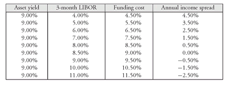
As 3-month LIBOR increases, the income spread decreases. If 3-month LIBOR exceeds 8.5%, the income spread is negative (i.e., it costs more to borrow than is earned on the bonds in which the borrowed funds are invested).
This financial institution has a mismatch between its assets and its liabilities. An interest rate swap can be used to hedge this mismatch. For example, suppose the manager of this financial institution enters into a 5-year swap with a $50 million notional amount in which it agrees to pay a fixed rate (i.e., to be the fixed-rate payer) in exchange for 3-month LIBOR. Suppose further that the swap rate is 6%. Then the annual income spread taking into account the swap payments is as follows for different values of 3-month LIBOR: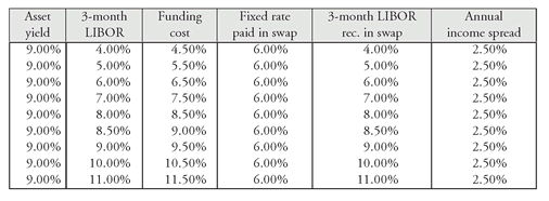

Assuming the bond does not default and is not called, the financial institution has locked in a spread of 250 basis points.
Effectively, the financial institution using this interest rate swap converted a fixed-rate asset into a floating-rate asset. The reference rate for the synthetic floating-rate asset is 3-month LIBOR and the liabilities are in terms of 3-month LIBOR. Alternatively, the financial institution could have converted its liabilities to a fixed-rate by entering into a 5-year $50 million notional amount swap by being the fixed-rate payer and the results would have been the same.
This simple illustration shows the critical importance of an interest rate swap. Investors and issuers with a mismatch of assets and liabilities can use an interest rate swap to better match assets and liabilities, thereby reducing their risk.
C. Determinants of the Swap Spread
Market participants throughout the world view the swap spread as the appropriate spread measure for valuation and relative value analysis. Here we discuss the determinants of the swap spread.
We know that
where Treasury rate is equal to the yield on a Treasury with the same maturity as the swap. Since the parties are swapping the future reference rate for the swap rate, then:
swap rate = Treasury rate + swap spread
reference rate = Treasury rate + swap spread
Solving for the swap spread we have:
swap spread = reference rate − Treasury rate
Since the most common reference rate is LIBOR, we can substitute this into the above formula getting:
swap spread = LIBOR − Treasury rate
Thus, the swap spread is a spread of the global cost of short-term borrowing over the Treasury rate.
EXHIBIT 8 Three-Year Trailing Correlation Between Swap Spreads and Credit Spreads (AA, A, and BB): June 1992 to December 2001
Source: Lehman Brothers Fixed Income Research, Global Fixed Income Strategy “Playbook,” January 2002.
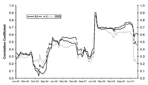
EXHIBIT 9 January and December 2001 Swap Spread Curves for Germany, Japan, U.K., and U.S.
Source: Lehman Brothers Fixed Income Research, Global Fixed Income Strategy “Playbook,” January 2002.

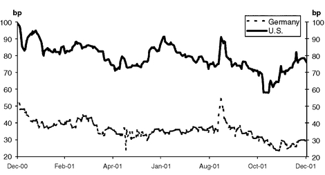
EXHIBIT 10 Daily 5-Year Swap Spreads in Germany and the United States: 2001
Source: Lehman Brothers Fixed Income Research, Global Fixed Income Strategy “Playbook,” January 2002.
The swap spread primarily reflects the credit spreads in the corporate bond market.45 Studies have found a high correlation between swap spreads and credit spreads in various sectors of the fixed income market. This can be seen in Exhibit 8 (on the previous page) which shows the 3-year trailing correlation from June 1992 to December 2001 between swap spreads and AA, A, and BBB credit spreads. Note from the exhibit that the highest correlation is with AA credit spreads.
D. Swap Spread Curve
A swap spread curve shows the relationship between the swap rate and swap maturity. A swap spread curve is available by country. The swap spread is the amount added to the yield of the respective country’s government bond with the same maturity as the maturity of the swap. Exhibit 9 shows the swap spread curves for Germany, Japan, the U.K., and the U.S. for January 2001 and December 2001. The swap spreads move together. For example, Exhibit 10 shows the daily 5-year swap spreads from December 2000 to December 2001 for the U.S. and Germany.
..................Content has been hidden....................
You can't read the all page of ebook, please click here login for view all page.
