CHAPTER 22
CONTROLLING INTEREST RATE RISK WITH DERIVATIVES347
I . INTRODUCTION
Previously, the features and characteristics of interest rate futures and swaps were explained. In addition, at Level II, the valuation of these derivative instruments was explained. In this chapter, our focus is on using derivatives to control the interest rate risk of a portfolio. Other uses for derivatives include speculating on interest rate movements and speculating on changes in interest rate volatility. These strategies are similar to those employed in the equity market and are not covered in this book.
II. CONTROLLING INTEREST RATE RISK WITH FUTURES
The price of an interest rate futures contract moves in the opposite direction from the change in interest rates: when rates rise, the futures price falls; when rates fall, the futures price rises. Buying a futures contract increases a portfolio’s exposure to a rate change. That is, the portfolio’s duration increases. Selling a futures contract decreases a portfolio’s exposure to a rate change. Equivalently, selling a futures contract that reduces the portfolio’s duration. Consequently, buying and selling futures can be used to alter the duration of a portfolio.
While managers can alter the duration of their portfolios with cash market instruments (buying or selling Treasury securities), using interest rate futures has the following four advantages:
Advantage 1: Transaction costs for trading futures are lower than trading in the cash market.
Advantage 2: Margin requirements are lower for futures than for Treasury securities; using futures thus permits greater leverage.
Advantage 3: It is easier to sell short in the futures market than in the cash market.
Advantage 4: Futures can be used to construct a portfolio with a longer duration than is available using cash market securities.
To appreciate the last advantage, suppose that in a certain interest rate environment a pension fund manager must structure a portfolio to have a duration of 15 to accomplish a particular investment objective. Bonds with such a long duration may not be available. By buying the appropriate number and kind of interest rate futures contracts, a pension fund manager can increase the portfolio’s duration to the target level of 15.
A. General Principles of Interest Rate Risk Control
The general principle in controlling interest rate risk with futures is to combine the dollar exposure of the current portfolio and the dollar exposure of a futures position so that the total dollar exposure is equal to the target dollar exposure. This means that the manager must be able to accurately measure the dollar exposure of both the current portfolio and the futures contract employed to alter the risk profile.
There are two commonly used measures for approximating the change in the dollar value of a bond or bond portfolio resulting from changes in interest rates: price value of a basis point (PVBP) and duration. PVBP is the dollar price change resulting from a one-basis-point change in yield. Duration is the approximate percentage change in price for a 100-basis-point change in rates. (Given the percentage price change, the dollar price change for a given change in interest rates can be computed.) There are two measures of duration: modified and effective. Effective duration is the appropriate measure for bonds with embedded options. In this chapter when we refer to duration, we mean effective duration. Moreover, since the manager is interested in dollar price exposure, the effective dollar duration should be used. For a one basis point change in rates, PVBP is equal to the effective dollar duration for a one-basis-point change in rates.
As emphasized in earlier chapters, a good valuation model is needed to estimate the effective dollar duration. The valuation model is used to determine the new values for the bonds in the portfolio if rates change. Consequently, the starting point in controlling interest rate risk is the development of a reliable valuation model. A reliable valuation model is also needed to value the derivative contracts that the manager wants to use to control interest rate exposure.
Suppose that a manager seeks a target duration for the portfolio based on either expectations of interest rates or client-specified exposure. Given the target duration, a target dollar duration for a small basis point change in interest rates can be computed. For a 50 basis point change in interest rates the target dollar duration can be found by multiplying the target duration by the dollar value of the portfolio and then dividing by 200. (We divide by 2 because we are dealing with one half of a 100 basis point change.) For example, suppose that the manager of a $500 million portfolio wants a target duration of 6. That is, the manager seeks a 3% change in the value of the portfolio for a 50 basis point change in rates (assuming a parallel shift in rates of all maturities). Multiplying the target duration of 6 by $500 million and dividing by 200 gives a target dollar duration of $15 million.
The manager must then determine the dollar duration of the current portfolio. The current dollar duration for a 50 basis point change in interest rates is calculated by multiplying the current duration by the dollar value of the portfolio and dividing by 200. For our $500 million portfolio, suppose that the current duration is 4. The current dollar duration is then $10 million (4 times $500 million divided by 200).
The target dollar duration is then compared to the current dollar duration; the difference is the dollar exposure that must be provided by a position in the futures contract. If the target dollar duration exceeds the current dollar duration, a futures position must increase the dollar exposure by the difference. To increase the dollar exposure, an appropriate number of futures contracts must be purchased. If the target dollar duration is less than the current dollar duration, an appropriate number of futures contracts must be sold. That is,
If target dollar duration - current dollar duration > 0, buy futures
If target dollar duration - current dollar duration < 0, sell futures
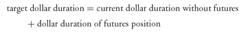
Once a futures position is taken, the portfolio’s dollar duration is equal to the sum of the current dollar duration without futures plus the dollar duration of the futures position. That is,
portfolio’s dollar duration = current dollar duration without futures + dollar duration of futures position
The objective is to control the portfolio’s interest rate risk by establishing a futures position such that the portfolio’s dollar duration is equal to the target dollar duration. Thus,
portfolio’s dollar duration = target dollar duration
Or, equivalently,
Over time, as interest rates change, the portfolio’s dollar duration will move away from the target dollar duration. The manager can alter the futures position to adjust the portfolio’s dollar duration back to the target dollar duration.
Our focus above is on duration. However, duration measures price sensitivity to changes in interest rates assuming a parallel shift in the yield curve. For bond portfolios, nonparallel shifts in the yield curve should be taken into account. The same is true for individual mortgage-backed securities because, as explained in the next chapter, these securities are sensitive to changes in the yield curve. In the next chapter, a framework will be presented that shows how to hedge both a change in the level of interest rates and a change in the shape of the yield curve.
1. Determining the Number of Contracts Each futures contract calls for delivery of a specified par value of the underlying instrument. When interest rates change, the market value of the underlying instrument changes, and therefore the value of the futures contract changes. The amount of change in the futures dollar value must be estimated. This amount is called the dollar duration per futures contract. For example, assume the price of an interest rate futures contract is 70 and that the underlying interest rate instrument has a par value of $100,000. Thus, the futures delivery price is $70,000 (0.70 times $100,000). Suppose that a change in interest rates of 100 basis points results in a futures price change of about 3% per contract. Then the dollar duration per futures contract is $2,100 (0.03 times $70,000).
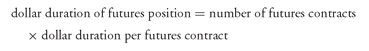
The dollar duration of a futures position is then the number of futures contracts multiplied by the dollar duration per futures contract. That is,
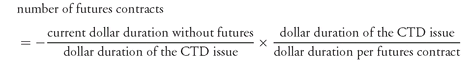
How many futures contracts are needed to obtain the target dollar duration? Substituting equation (2) into equation (1), we get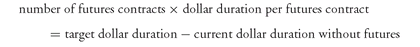
(3)
Solving for the number of futures contracts we have:
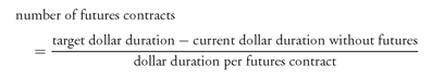
Equation (4) gives the approximate number of futures contracts needed to adjust the portfolio’s dollar duration to the target dollar duration. A positive number means that futures contracts must be purchased; a negative number means that futures contracts must be sold. Notice that if the target dollar duration is greater than the current dollar duration without futures, the numerator is positive and futures contracts are purchased. If the target dollar duration is less than the current dollar duration without futures, the numerator is negative and futures contracts are sold.
2. Dollar Duration for a Futures Position Now we discuss how to measure the dollar duration of a bond futures position. Keep in mind that the goal is to measure the sensitivity of the bond futures value to a change in rates.
Given a valuation model, the general methodology for computing the dollar duration of a futures position for a given change in interest rates is straightforward. The procedure is used for computing the dollar duration of any cash market instrument—shock (change) interest rates up and down by the same number of basis points and compute the average dollar price change.
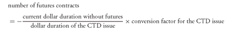
An adjustment is needed for the Treasury bond and note futures contracts. As explained, the pricing of the futures contract depends on the cheapest-to-deliver (CTD) issue.348The calculation of the dollar duration of a Treasury bond or note futures contract requires computing the effect of a change in interest rates on the price of the CTD issue, which in turn determines the change in the futures price. The dollar duration of a Treasury bond and note futures contract is determined as follows: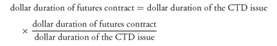
Recall that a conversion factor is specified for each issue that is acceptable for delivery under the futures contract. For each deliverable issue, the product of the futures price and the conversion factor is the adjusted futures price for the issue. This adjusted price is called the converted price. Relating this to the equation above, the second term is approximately equal to the reciprocal of the conversion factor of the cheapest-to-deliver issue. Thus, we can write: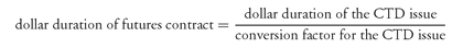
B. Hedging with Interest Rate Futures
Hedging with futures calls for taking a futures position as a temporary substitute for transactions to be made in the cash market at a later date. If cash and futures prices are perfectly positively correlated, any loss realized by the hedger from one position (whether cash or futures) will be exactly offset by a profit on the other position. Hedging is a special case of controlling interest rate risk. In a hedge, the manager seeks a target duration or target dollar duration of zero.
A short hedge (or sell hedge) is used to protect against a decline in the cash price of a bond. To execute a short hedge, futures contracts are sold. By establishing a short hedge, the manager has fixed the future cash price and transferred the price risk of ownership to the buyer of the futures contract. To understand why a short hedge might be executed, suppose that a pension fund manager knows that bonds must be liquidated in 40 days to make a $5 million payment to beneficiaries. If interest rates rise during the 40-day period, more bonds will have to be liquidated at a lower price than today to realize $5 million. To guard against this possibility, the manager can lock in a selling price by selling bonds in the futures market.349
A long hedge (or buy hedge) is undertaken to protect against an increase in the cash price of a bond. In a long hedge, the manager buys a futures contract to lock in a purchase price. A pension fund manager might use a long hedge when substantial cash contributions are expected and the manager is concerned that interest rates will fall. Also, a money manager who knows that bonds are maturing in the near future and expects that interest rates will fall before receipt can employ a long hedge to lock in a rate for the proceeds to be reinvested.
In bond portfolio management, typically the bond or portfolio to be hedged is not identical to the bond underlying the futures contract. This type of hedging is referred to as cross hedging.
The hedging process can be broken down into four steps:
Step 1: Determining the appropriate hedging instrument.
Step 2: Determining the target for the hedge.
Step 3: Determining the position to be taken in the hedging instrument.
Step 4: Monitoring and evaluating the hedge.
We discuss each step below.
1. Determining the Appropriate Hedging Instrument A primary factor in determining which futures contract will provide the best hedge is the correlation between the price on the futures contract and the interest rate that creates the underlying risk that the manager seeks to eliminate. For example, a long-term corporate bond portfolio can be better hedged with Treasury bond futures than with Treasury bill futures because long-term corporate bond rates are more highly correlated with Treasury bond futures than Treasury bill futures. Using the correct delivery month is also important. A manager trying to lock in a rate or price for September will use September futures contracts because they will give the highest degree of correlation.
Correlation is not, however, the only consideration if the hedging program is of significant size. If, for example, a manager wants to hedge $600 million of a cash position in a distant delivery month, liquidity becomes an important consideration. In such a case, it might be necessary for the manager to spread the hedge across two or more different contracts.
While our focus in this chapter is on hedging changes in the level of interest rates, when more than one type of change in the yield curve is to be hedged, then more than one hedging instrument must be used. For example, hedging a mortgage security is covered in the next chapter. As explained in the next chapter, because of the characteristic of mortgage securities, hedging both a change in the level and slope of the yield curve would be more effective. In such cases, two hedging instruments are used. One can also hedge the level, slope, and curvature changes of the yield curve. In that case, three hedging instruments are used.
2. Determining the Target for the Hedge Having determined the correct contract and the correct delivery months, the manager should then determine what is expected from the hedge—that is, what rate will, on average, be locked in by the hedge. This is the target rate or target price. If this target rate is too high (if hedging a future sale) or too low (if hedging a future purchase), hedging may not be the right strategy for dealing with the unwanted risk. Determining what is expected (calculating the target rate or price for a hedge) is not always simple. We’ll see how a manager should approach this problem for both simple and complex hedges.
a. Risk and Expected Return in a Hedge When a manager enters into a hedge, the objective is to “lock in” a rate for the sale or purchase of a security. However, there is much disagreement about which rate or price a manager should expect to lock in when futures are used to hedge. Here are the two views:
View 1: The manager can, on average, lock in the rate at which the futures contracts are bought or sold.
View 2: The manager can, on average, lock in the current spot rate for the security (i.e., current rate in the cash market).
Reality usually lies somewhere between these two views. However, as the following cases illustrate, each view is appropriate for certain situations.
b. The Target for Hedges Held to Delivery Hedges that are held until the futures delivery date provide an example of a hedge that locks in the futures rate (i.e., the first view). The futures rate is the interest rate corresponding to the futures delivery price of the deliverable instrument. The complication in the case of using Treasury bond futures and Treasury note futures to hedge the value of intermediate- and long-term bonds, is that because of the delivery options the manager does not know for sure when delivery will take place or which bond will be delivered. This is because of the delivery options granted to the short.350
To illustrate how a Treasury bond futures contract held to the delivery date locks in the futures rate, assume for the sake of simplicity that the manager knows which Treasury bond will be delivered and that delivery will take place on the last day of the delivery month. Suppose that for delivery on the September 1999 futures contract, the conversion factor for a deliverable Treasury issue—the of 2/15/15—is 1.283, implying that the investor who delivers this issue would receive from the buyer 1.283 times the futures settlement price plus accrued interest. An important principle to remember is that at delivery, the spot price and the futures price times the conversion factor must converge. Convergence refers to the fact that at delivery there can be no discrepancy between the spot price and futures price for a given security. If convergence does not take place, arbitrageurs would buy at the lower price and sell at the higher price and earn risk-free profits. Accordingly, a manager could lock in a September 1999 sale price for this issue by selling Treasury bond futures contracts equal to 1.283 times the par value of the bonds. For example, $100 million face value of this issue would be hedged by selling $128.3 million face value of bond futures (1,283 contracts).
The sale price that the manager locks in would be 1.283 times the futures price. This is the converted price. Thus, if the futures price is 113 when the hedge is set, the manager locks in a sale price of 144.979 (113 times 1.283) for September 1999 delivery, regardless of where rates are in September 1999. Exhibit 1 shows the cash flows for various final prices for this issue and illustrates how cash flows on the futures contracts offset gains or losses relative to the target price of 144.979.
Let’s look at each of the columns in Exhibit 1 and explain the computations for one of the scenarios—that is, for one actual sale price for the  of 2/15/15 Treasury issue. Consider the first actual sale price of 140. By convergence, at the delivery date the final futures price shown in Column (2) must equal the Treasury bond’s actual sale price adjusted by the conversion factor. Thus, the final futures price in Column (2) of Exhibit 1 is computed as follows:
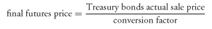
Since the conversion factor is 1.283 for the  of 2/15/15 Treasury issue, for the first actual sale price of 140, the final futures price is
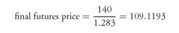
Column (3) shows the market value of the Treasury bonds. This is found by dividing the actual sale price in Column (1) by 100 to obtain the actual sale price per $1 of par value and then multiplying by the $100 million par value. That is,
market value of Treasury bonds = (actual sale price/100) × $100, 000, 000
For the actual sale price of 140, the value in Column (3) is
market value of Treasury bonds = (140/100) × $100, 000, 000 = $140, 000, 000
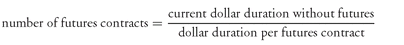
Column (4) shows the value of the futures position at the delivery date. This value is computed by first dividing the futures price shown in Column (2) by 100 to obtain the futures price per $1 of par value. Then this value is multiplied by the par value per contract of $100,000 and further multiplied by the number of futures contracts. That is,
value of futures position = (final futures price/100) × $100, 000 × number of futures contracts
EXHIBIT 1 Treasury Issue Hedge Held to Delivery
In our illustration, the number of futures contracts is 1,283. For the actual sale price of the bond at 140, the final futures price calculated earlier is 109.1193. So, the value shown in Column (4) is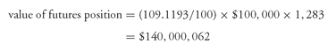
The value shown in Column (4) is $140,000,000 because the final futures price of 109.1193 was rounded. Using more decimal places the value would be $140,000,000.
Now let’s look at the gain or loss from the futures position. This value is shown in Column (5). Recall that the futures contract was shorted. The futures price at which the contracts were sold was 113. So, if the final futures price exceeds 113, this means that there is a loss on the futures position—that is, the futures contract is purchased at a price greater than that at which it was sold. In contrast, if the futures price is less than 113, this means that there is a gain on the futures position—that is, the futures contract is purchased at a price less than that at which it was sold. The gain or loss is determined by the following formula:
([113 - final futures price]/100) × $100, 000 × number of futures contracts
In our illustration, for a final futures price of 109.1193 and 1,283 futures contracts, we have
([113 - 109.1193]/100) × $100, 000 × 1, 283 = $4, 978, 938.1
The value shown in Column (5) is $4,979,000 because that is the more precise value using more decimal places for the final futures price than shown in Exhibit 1. The value is positive indicating a gain in the futures position. Note that for all the final futures prices above 113 in Exhibit 1, there is a negative value which means that there is a loss on the futures position.
Finally, Column (6) shows the effective sale price for the Treasury bond. This value is computed as follows:
which is the sum of the numbers in each of the rows of Columns (3) and (5). For the actual sale price of $140 million, the gain is $4,979,000. Therefore the effective sale price for the Treasury bond is
effective sale price for Treasury bond = actual sale price of Treasury bond
+ gain or loss on futures position
+ gain or loss on futures position
$140, 000, 000 + $4,979,000 = $144, 979, 000
Note that this is the target price for the Treasury bond. In fact, it can be seen from Column (6) of Exhibit 1 that the effective sale price for all the actual sale prices for the Treasury bond is the target price. However, the target price is determined by the futures price, so the target price may be higher or lower than the cash (spot) market price when the hedge is set.
When we admit the possibility that bonds other than the issue used in our illustration can be delivered, and that it might be advantageous to do so, the situation becomes somewhat more involved. In this more realistic case, the manager may decide not to deliver this issue, but if she does decide to deliver it, the manager is still assured of receiving an effective sale price of approximately 144.979. If the manager does not deliver this issue, it would be because another issue can be delivered more cheaply, and thus the manager does better than the targeted price.
In summary, if a manager establishes a futures hedge that is held until delivery, the manager can be assured of receiving an effective price dictated by the futures rate (not the spot rate) on the day the hedge is set.
c. The Target for Hedges with Short Holding Periods When a manager must lift (remove) a hedge prior to the delivery date, the effective rate that is obtained is more likely to approximate the current spot rate than the futures rate and this likelihood increases the shorter the term of the hedge. The critical difference between this hedge and the hedge held to the delivery date is that convergence will generally not take place by the termination date of the hedge.
To illustrate why a manager should expect the hedge to lock in the spot rate rather than the futures rate for very short-lived hedges, let’s return to the simplified example used earlier to illustrate a hedge maintained to the delivery date. It is assumed that this issue is the only deliverable instrument for the Treasury bond futures contract. Suppose that the hedge is set three months before the delivery date and the manager plans to lift the hedge one day later. It is much more likely that the spot price of the bond will move parallel to the converted futures price (that is, the futures price times the conversion factor), than that the spot price and the converted futures price will converge by the time the hedge is lifted.
A 1-day hedge is, admittedly, an extreme example. Other than underwriters, dealers, and traders who reallocate assets very frequently, few money managers are interested in such a short horizon. The very short-term hedge does, however, illustrate a very important point: when hedging, a manager should not expect to lock in the futures rate (or price) just by hedging with futures contracts. The futures rate is locked in only if the hedge is held until delivery, at which point convergence must take place. If the hedge is held for only one day, the manager should expect to lock in the 1-day forward rate,351 which will very nearly equal the spot rate. Generally hedges are held for more than one day, but not necessarily to delivery.
d. How the Basis Affects the Target Rate for a Hedge The proper target for a hedge that is to be lifted prior to the delivery date depends on the basis. The basis is simply the difference between the spot (cash) price of a security and its futures price; that is:
basis = spot price - futures price
In the bond market, a problem arises when trying to make practical use of the concept of the basis. The quoted futures price does not equal the price that one receives at delivery. For the Treasury bond and note futures contracts, the actual futures price equals the quoted futures price times the appropriate conversion factor. Consequently, to be useful, the basis in the bond market should be defined using actual futures delivery prices rather than quoted futures prices. Thus, the price basis for bonds should be redefined as:
price basis = spot price - futures delivery price
For hedging purposes it is also frequently useful to define the basis in terms of interest rates rather than prices. The rate basis is defined as:
rate basis = spot rate - futures rate
where spot rate refers to the current rate on the instrument to be hedged and the futures rate is the interest rate corresponding to the futures delivery price of the deliverable instrument.
The rate basis is helpful in explaining why the two views of hedging described earlier are expected to lock in such different rates. To see this, we first define the target rate basis. This is defined as the expected rate basis on the day the hedge is lifted. That is,
target rate basis = spot rate on date hedge is lifted - futures rate on date hedge is lifted
The target rate for the hedge is equal to
target rate for hedge = futures rate + target rate basis
Substituting for target rate basis in the above equation
target rate for hedge = futures rate + spot rate on date hedge is lifted
- futures rate on date hedge is lifted
- futures rate on date hedge is lifted
Consider first a hedge lifted on the delivery date. On the delivery date, the spot rate and the futures rate will be the same by convergence. Thus, the target rate basis if the hedge is expected to be removed on the delivery date is zero. Substituting zero for the target rate basis in the equation above we have the following:
target rate for hedge = futures rate
That is, if the hedge is held to the delivery date, the target rate for the hedge is equal to the futures rate.
Now consider if a hedge is lifted prior to the delivery date. Let’s consider the case where the hedge is removed the next day. One would not expect the basis to change very much in one day. Assume that the basis does not change. Then,
spot rate on date hedge is lifted = spot rate when hedge was placed
futures rate on date hedge is lifted = futures rate when hedge was placed
The spot rate when the hedge was placed is simply the spot rate and the futures rate when the hedge was placed is simply the futures rate. So, we can write
and substituting the right-hand side of the equation into the target rate for hedge
or
target rate basis = spot rate - futures rate
target rate for hedge = futures rate + (spot rate - futures rate)
target rate for hedge = spot rate
Thus, we see that when hedging for one day (and assuming the basis does not change in that one day), the manager is locking in the spot rate (i.e., the current rate).
If projecting the basis in terms of price rather than rate is easier (as is often the case for intermediate- and long-term futures), it is easier to work with the target price basis instead of the target rate basis. The target price basis is the projected price basis for the day the hedge is to be lifted. For a deliverable security, the target for the hedge then becomes
target price for hedge = futures delivery price + target price basis
The idea of a target price or rate basis explains why a hedge held until the delivery date locks in a price, and other hedges do not. The examples have shown that this is true. For the hedge held to delivery, there is no uncertainty surrounding the target basis; by convergence, the basis on the day the hedge is lifted will be zero. For the short-lived hedge, the basis will probably approximate the current basis when the hedge is lifted, but its actual value is not known in advance. For hedges longer than one day but ending prior to the futures delivery date, there can be considerable basis risk because the basis on the day the hedge is lifted can end up being anywhere within a wide range. Thus, the uncertainty surrounding the outcome of a hedge is directly related to the uncertainty surrounding the basis on the day the hedge is lifted (i.e., the uncertainty surrounding the target basis).
The uncertainty about the value of the basis at the time the hedge is removed is called basis risk. For a given investment horizon, hedging substitutes basis risk for price risk. Thus, one trades the uncertainty of the price of the hedged security for the uncertainty of the basis. A manager would be willing to substitute basis risk for price risk if the manager expects that basis risk is less than price risk. Consequently, when hedges do not produce the desired results, it is common to place the blame on basis risk. However, basis risk is the real culprit only if the target for the hedge is properly defined. Basis risk should refer only to the unexpected or unpredictable part of the relationship between cash and futures prices. The fact that this relationship changes over time does not in itself imply that there is basis risk.
Basis risk, properly defined, refers only to the uncertainty associated with the target rate basis or target price basis. Accordingly, it is imperative that the target basis be properly defined if one is to correctly assess the risk and expected return in a hedge.
3. Determining the Position to Be Taken The final step that must be determined before the hedge is set is the number of futures contracts needed for the hedge. This is called the hedge ratio. Usually the hedge ratio is expressed in terms of relative par amounts. Accordingly, a hedge ratio of 1.20 means that for every $1 million par value of securities to be hedged, one needs $1.2 million par value of futures contracts to offset the risk. In our discussion, the values are defined so that the hedge ratio is the number of futures contracts.
Earlier, we defined a cross hedge in the futures market as a hedge in which the security to be hedged is not deliverable on the futures contract used in the hedge. (A bond that does not meet the specific criteria for delivery to satisfy a particular futures contract is referred to as a nondeliverable bond.) For example, a manager who wants to hedge the sale price of long-term corporate bonds might hedge with the Treasury bond futures contract, but since non-Treasury bonds cannot be delivered in satisfaction of the contract, the hedge would be considered a cross hedge. A manager might also want to hedge a rate that is of the same quality as the rate specified in one of the contracts, but that has a different maturity. For example, it might be necessary to cross hedge a Treasury bond, note, or bill with a maturity that does not qualify for delivery on any futures contract. Thus, when the security to be hedged differs from the futures contract specification in terms of either quality or maturity, one is led to the cross hedge.
Conceptually, cross hedging is somewhat more complicated than hedging deliverable securities, because it involves two relationships. First, there is the relationship between the cheapest-to-deliver (CTD) issue and the futures contract. Second, there is the relationship between the security to be hedged and the CTD issue. Practical considerations may at times lead a manager to shortcut this two-step relationship and focus directly on the relationship between the security to be hedged and the futures contract, thus ignoring the CTD issue altogether. However, in so doing, a manager runs the risk of miscalculating the target rate and the risk in the hedge. Furthermore, if the hedge does not perform as expected, the shortcut makes it difficult to tell why the hedge did not work out as expected.
The key to minimizing risk in a cross hedge is to choose the right number of futures contracts. This depends on the relative dollar duration of the bond to be hedged and the dollar duration of the futures position. Equation (4) indicated the number of futures contracts required to achieve a particular target dollar duration. The objective in hedging is to make the target dollar duration equal to zero. Substituting zero for target dollar duration in equation (4) we obtain:
To calculate the dollar duration of a bond, the manager must know the precise point in time that the dollar duration is to be calculated (because price volatility generally declines as a bond matures) as well as the price or yield at which to calculate dollar duration (because higher yields generally reduce dollar duration for a given yield change). The relevant point in the life of the bond for calculating price volatility is the point at which the hedge will be lifted. Dollar duration at any other point in time is essentially irrelevant because the goal is to lock in a price or rate only on that particular day. Similarly, the relevant yield at which to calculate dollar duration initially is the target yield. Consequently, the numerator of equation (5) is the dollar duration on the date the hedge is expected to be lifted. The yield that can be used on this date in order to determine the dollar duration is the forward rate.
Let’s look at how we apply equation (5) when using the Treasury bond futures contract to hedge. The number of futures contracts will be affected by the dollar duration of the CTD issue. We can modify equation (5) as follows:
As noted earlier, the conversion ratio for the CTD issue is a good approximation of the second ratio. Thus, equation (6) can be rewritten as
a. An Illustration An example for a single bond shows why dollar duration weighting leads to the correct number of contracts for a hedge. The hedge illustrated is a cross hedge. Suppose that on 6/24/99, a manager owned $10 million par value of a 6.25% Fannie Mae (FNMA) option-free bond maturing on 5/15/29 selling at 88.39 to yield 7.20%. The manager wants to sell September 1999 Treasury bond futures to hedge a future sale of the FNMA bond. At the time, the price of the September Treasury bond futures contract was 113. The CTD issue was the 11.25% of 2/15/15 issue that was trading at 146.19 to yield 6.50%. The conversion factor for the CTD issue was 1.283. To simplify, assume that the yield spread between the FNMA bond and the CTD issue remains at 0.70% (i.e., 70 basis points) and that the anticipated sale date is the last business day in September 1999.
The target price for hedging the CTD issue would be 144.979 (113 × 1.283), and the target yield would be 6.56% (the yield at a price of 144.979). Since the yield on the FNMA bond is assumed to stay at 0.70% above the yield on the CTD issue, the target yield for the FNMA bond would be 7.26%. The corresponding price for the FNMA bond for this target yield is 87.76. At these target levels, the dollar durations for a 50 basis point change in rates for the CTD issue and the FNMA bond per $100 of par value are $6.255 and $5.453, respectively. As indicated earlier, all these calculations are made using a settlement date equal to the anticipated sale date, in this case the end of September 1999. The dollar duration for a 50 basis point change in rates for $10 million par value of the FNMA bond is then $545,300 ([$10 million/100] × $5.453). Per $100,000 par value for the CTD issue, the dollar duration per futures contract is $6,255 ([$100,000/100] × $6.255).
Thus, we know current dollar duration without futures = dollar duration of the FNMA bond = $545, 300
dollar duration of the CTD issue = $6,255
conversion factor for CTD issue = 1.283
Substituting these values into equation (7) we obtain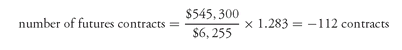
Consequently, to hedge the FNMA bond position, 112 Treasury bond futures contracts must be shorted.
Exhibit 2 uses scenario analysis to show the outcome of the hedge based on different prices for the FNMA bond at the delivery date of the futures contract. Let’s go through each of the columns. Column (1) shows the assumed sale price for the FNMA bond and Column (2) shows the corresponding yield based on the actual sale price in Column (1). This yield is found from the price/yield relationship. Column (3) shows the yield for the CTD issue, computed on the assumed 70 basis point yield spread between the FNMA bond and CTD issue. So, by subtracting 70 basis points from the yield for the FNMA bond in Column (2), the yield on the CTD issue (the 11.25% of 2/15/15) is obtained. Given the yield for the CTD issue in Column (3), the price per $100 of par value of the CTD issue can be computed. This CTD price is shown in Column (4).
Now we move from the price of the CTD issue to the futures price. As explained in the description of the columns in Exhibit 1, the futures price is computed by dividing the price for the CTD issue shown in Column (4) by the conversion factor of the CTD issue (1.283). This price is shown in Column (5).
EXHIBIT 2 Hedging a Nondeliverable Bond to a Delivery Date with Futures
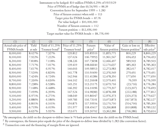
The value of the futures position is found in the same way as in Exhibit 1. First the futures price per $1 of par value is computed by dividing the futures price by 100. Then this value is multiplied by $100,000 (the par value for the contract) and the number of futures contracts. That is,
value of futures position = (futures price/100) × $100, 000 × number of futures contracts
The values in Column (6) are derived using this formula. Using the first sale price for the FNMA of $8 million as an example, the corresponding futures price in Column (5) is 105.8551. Since the number of futures contracts sold is 112, the value of the futures position is
value of futures position = (105.8551/100) × $100, 000 × 112 = $11, 855, 711
Now let’s calculate the gain or loss on the futures position shown in Column (7). Note that the negative values in Column (7) for all futures prices above 113 mean there is a loss on the futures position. Since the futures price at which the contracts are sold at the inception of the hedge is 113, the gain or loss on the futures position is found as follows:
([113 - final futures price]/100) × $100, 000 × number of futures contracts
For example, for the first scenario in Exhibit 2, the futures price is 105.8551 and 112 futures contract were sold. Therefore,
([113 - 105.8551]/100) × $100, 000 × 112 = $800, 229
There is a gain from the futures position because the futures price is less than 113. Note that for all the final futures prices above 113 in Exhibit 2, there is a negative value which means that there is a loss on the futures position. For all futures prices below 113, there is a gain.
Finally, Column (8) shows the effective sale price for the FNMA bond. This value is found as follows:
effective sale price for FNMA bond = actual sale price of FNMA bond
+ gain or loss on futures position
+ gain or loss on futures position
For the actual sale price of $8 million, the gain is $800,229. Therefore the effective sale price for the FNMA bond is
$8, 000, 000 + $800,229 = $8, 800, 229
Looking at Column (8) of Exhibit 2 we see that if the simplifying assumptions hold, a futures hedge using the recommended number of futures contracts (112) very nearly locks in the target price for $10 million par value of the FNMA bonds.
b. Refining for Changing Yield Spread Another refinement in the hedging strategy is usually necessary when hedging nondeliverable securities. This refinement concerns the assumption about the relative yield spread between the CTD issue and the bond to be hedged. In the prior discussion, we assumed that the yield spread was constant over time. Yield spreads, however, are not constant over time. They vary with the maturity of the instruments in question and the level of rates, as well as with many unpredictable and nonsystematic factors.
Regression analysis allows the manager to capture the relationship between yield levels and yield spreads and use it to advantage. For hedging purposes, the variables are the yield on the bond to be hedged and the yield on the CTD issue. The regression equation takes the form:
(8)
The regression procedure provides an estimate of b, which is the expected relative yield change in the two bonds. This parameter b is called the yield beta. Our example that used constant spreads implicitly assumes that the yield beta, b, equals l.0 and a equals 0.70 (because 0.70 is the assumed spread).
For the two issues in question, the FNMA bond and the CTD issue, suppose the estimated yield beta is 1.05. Thus, yields on the FNMA issue are expected to move 5% more than yields on the Treasury issue. To calculate the number of futures contracts correctly, this fact must be taken into account; thus, the number of futures contracts derived in our earlier example is multiplied by the factor 1.05. Consequently, instead of shorting 112 Treasury bond futures contracts to hedge $10 million of the FNMA bond, the investor would short 118 (rounded up) contracts.
To incorporate the impact of a yield beta, the formula for the number of futures contracts is revised as follows: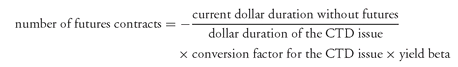
(9)
The effect of a change in the CTD issue and the yield spread can be assessed before the hedge is implemented. An exhibit similar to Exhibit 2 can be constructed under a wide range of assumptions. For example, at different yield levels at the date the hedge is to be lifted (the second column in Exhibit 2), a different yield spread may be appropriate and a different acceptable issue will be the CTD issue. The manager can determine what this will do to the outcome of the hedge.
4. Monitoring and Evaluating the Hedge After a target is determined and a hedge is set, there are two remaining tasks. The hedge must be monitored during its life and evaluated after it is over. While hedges must be monitored, overactive management of a hedge poses more of a threat to most hedges than does inactive management. The reason for this is that the manager usually will not receive enough new information during the life of the hedge to justify a change in the hedging strategy. For example, it is not advisable to readjust the hedge ratio every day in response to new data and a possible corresponding change in the estimated value of the yield beta.
There are, however, exceptions to this general rule. As rates change, dollar duration changes. Consequently, the hedge ratio may change slightly. In other cases, there may be sound economic reasons to believe that the yield beta has changed. While there are exceptions, the best approach is usually to let a hedge run its course using the original hedge ratio with only slight adjustments.
A hedge can normally be evaluated only after it has been lifted. Evaluation involves, first, an assessment of how closely the hedge locked in the target rate—that is, how much error there was in the hedge. To provide a meaningful interpretation of the error, the manager should calculate how far from the target the sale (or purchase) would have been, had there been no hedge at all. One good reason for evaluating a completed hedge is to ascertain the sources of error in the hedge in the hope that the manager will gain insights that can be used to advantage in subsequent hedges. A manager will find that there are three major sources of hedging errors:
1. The dollar duration for the hedged instrument was incorrect.
2. The projected value of the basis at the date the hedge is removed can be in error.
3. The parameters estimated from the regression (a and b) can be inaccurate.
Let’s discuss the first two sources of hedging error. The third source is self-explanatory. Recall from the calculation of duration that interest rates are changed up and down by a small number of basis points and the security is revalued. The two recalculated values are used in the numerator of the duration formula. The first source of error listed above recognizes that the instrument to be hedged may be a complex instrument (i.e., one with embedded options) and that the valuation model does not do a good job of valuing the security when interest rates change.
The second major source of errors in a hedge—an inaccurate projected value of the basis—is a more difficult problem. Unfortunately, there are no satisfactory easy models like regression analysis that can be applied to the basis. Simple models of the basis violate certain equilibrium relationships for bonds that should not be violated. On the other hand, theoretically rigorous models are very unintuitive and usually solvable only by complex numerical methods. Modeling the basis is undoubtedly one of the most important and difficult problems that managers face when seeking to hedge.
III. CONTROLLING INTEREST RATE RISK WITH SWAPS
An interest rate swap is equivalent to a package of forward/futures contracts. Consequently, swaps can be used for controlling interest rate risk and hedging as we discussed earlier with futures.
A. Hedging Interest Rate Risk
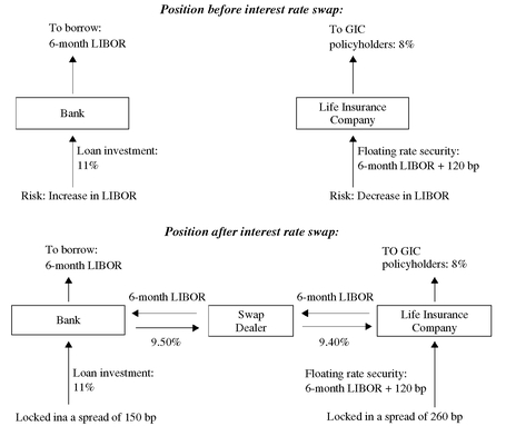
The following illustration demonstrates how an interest rate swap can be used to hedge interest rate risk by altering the cash flow characteristics of an entity so as to better match the cash flow characteristics of assets and liabilities. In our illustration we will use two hypothetical financial institutions—a commercial bank and a life insurance company.
Suppose a bank has a portfolio consisting of 4-year commercial loans with a fixed interest rate. The principal value of the portfolio is $100 million, and the interest rate on every loan in the portfolio is 11%. The loans are interest-only loans; interest is paid semiannually, and the principal is paid at the end of four years. That is, assuming no default on the loans, the cash flow from the loan portfolio is $5.5 million every six months for the next four years and $100 million at the end of four years. To fund its loan portfolio, assume that the bank can borrow at 6-month LIBOR for the next four years.
The risk that the bank faces is that 6-month LIBOR will be 11% or greater. To understand why, remember that the bank is earning 11% annually on its commercial loan portfolio. If 6-month LIBOR is 11% when the borrowing rate for the bank’s loan resets, there will be no spread income for that 6-month period. Worse, if 6-month LIBOR rises above 11%, there will be a loss for that 6-month period; that is, the cost of funds will exceed the interest rate earned on the loan portfolio. The bank’s objective is to lock in a spread over the cost of its funds.
The other party in the interest rate swap illustration is a life insurance company that has committed itself to pay an 8% rate for the next four years on a $100 million guaranteed investment contract (GIC) it has issued. Suppose that the life insurance company has the opportunity to invest $100 million in what it considers an attractive 4-year floating-rate instrument in a private placement transaction. The interest rate on this instrument is 6-month LIBOR plus 120 basis points. The coupon rate is set every six months.
The risk that the life insurance company faces in this instance is that 6-month LIBOR will fall so that the company will not earn enough to realize a spread over the 8% rate that it has guaranteed to the GIC policyholders. If 6-month LIBOR falls to 6.8% or less at a coupon reset date, no spread income will be generated. To understand why, suppose that 6-month LIBOR is 6.8% at the date the floating-rate instrument resets its coupon. Then the coupon rate for the next six months will be 8% (6.8% plus 120 basis points). Because the life insurance company has agreed to pay 8% on the GIC policy, there will be no spread income. Should 6-month LIBOR fall below 6.8%, there will be a loss for that 6-month period.
We can summarize the asset/liability problems of the bank and the life insurance company as follows.
Bank:
1. has lent long term and borrowed short term
2. if 6-month LIBOR rises, spread income declines
Life insurance company:
1. has lent short term and borrowed long term
2. if 6-month LIBOR falls, spread income declines
Now suppose the market has available a 4-year interest rate swap with a notional amount of $100 million, with the following swap terms available to the bank:
1. every six months the bank will pay 9.50% (annual rate)
2. every six months the bank will receive LIBOR
Suppose the swap terms available to the insurance company are as follows:
1. every six months the life insurance company will pay LIBOR
2. every six months the life insurance company will receive 9.40%
Now let’s look at the positions of the bank and the life insurance company after the swap. Exhibit 3 summarizes the position of each institution before and after the swap. Consider first the bank. For every 6-month period for the life of the swap, the interest rate spread will be as follows:
| Annual interest rate received: | ||
|---|---|---|
| commercial loan portfolio | = | 11.00% |
| From interest rate swap | = | 6-month LIBOR |
| Total | = | 11.00%+ 6-month LIBOR |
EXHIBIT 3 Position of Bank and Life Insurance Company Before and After Swap
| Annual interest rate paid: | ||
|---|---|---|
| To borrow funds | = | 6-month LIBOR |
| On interest rate swap | = | 9.50% |
| Total | = | 9.50%+ 6-month LIBOR |
| Outcome: | ||
|---|---|---|
| To be received | = | 11.0% + 6-month LIBOR |
| To be paid | = | 9.50% + 6-month LIBOR |
| Spread income | = | 1.50% or 150 basis points |
Thus, regardless of changes in 6-month LIBOR, the bank locks in a spread of 150 basis points assuming no loan defaults or payoffs.
Now let’s look at the effect of the interest rate swap on the life insurance company:
| Annual interest rate received: | ||
|---|---|---|
| floating-rate instrument | = | 1.20% + 6-month LIBOR |
| From interest rate swap | = | 9.40% |
| Total | = | 10.60% + 6-month LIBOR |
| Annual interest rate paid: | ||
|---|---|---|
| To GIC policyholders | = | 8.00% |
| On interest rate swap | = | 6-month LIBOR |
| Total | = | 8.00% + 6-month LIBOR |
| Outcome: | ||
|---|---|---|
| be received | = | 10.60% + 6-month LIBOR |
| To be paid | = | 8.00% + 6-month LIBOR |
| Spread income | = | 2.60% or 260 basis points |
Regardless of what happens to 6-month LIBOR, the life insurance company locks in a spread of 260 basis points assuming the issuer of the floating-rate instrument does not default.
The interest rate swap has allowed each party to accomplish its asset/liability objective of locking in a spread.352 It permits the two financial institutions to alter the cash flow characteristics of its assets: from fixed to floating in the case of the bank, and from floating to fixed in the case of the life insurance company.
B. Dollar Duration of a Swap
Effectively, a position in an interest rate swap is a leveraged position. This agrees with the economic interpretations of an interest rate swap explained earlier. We know that futures/forwards are leveraged instruments. In the case of a package of cash instruments, it is a leveraged position involving either buying a fixed-rate bond and financing it on a floating-rate basis (i.e., fixed-rate receiver position) or buying a floating-rate bond on a fixed-rate basis (i.e., fixed-rate payer position). So, we would expect that the dollar duration of a swap is a multiple of the bond that effectively underlies the swap.
To see how to calculate the dollar duration, let’s work with the second economic interpretation of a swap—a package of cash flows from buying and selling cash market instruments. From the perspective of the fixed-rate receiver, the position can be viewed as follows:
long a fixed-rate bond + short a floating-rate bond
The fixed-rate bond is a bond with a coupon rate equal to the swap rate, a maturity equal to the term of the swap, and a par value equal to the notional amount of the swap.
This means that the dollar duration of an interest rate swap from the perspective of a fixed-rate receiver is the difference between the dollar durations of the two bond positions that comprise the swap. That is,
dollar duration of a swap for a fixed-rate receiver
= dollar duration of a fixed-rate bond - dollar duration of a floating-rate bond
= dollar duration of a fixed-rate bond - dollar duration of a floating-rate bond
Most of the swap’s interest rate sensitivity results from the dollar duration of the fixed-rate bond since the dollar duration of the floating-rate bond will be small. The dollar duration of a floating-rate bond is smaller the closer the swap is to its reset date. If the dollar duration of the floating-rate bond is close to zero then:
dollar duration of a swap for a fixed-rate receiver ≈ dollar duration of a fixed-rate bond
Thus, adding an interest rate swap to a portfolio in which the manager pays a floating-rate and receives a fixed-rate increases the dollar duration of the portfolio by roughly the dollar duration of the underlying fixed-rate bond. This is because it effectively involves buying a fixed-rate bond on a leveraged basis.
We can use the cash market instrument economic interpretation to compute the dollar duration of a swap for the fixed-rate payer. The dollar duration is:
dollar duration of a swap for a fixed-rate payer
= dollar duration of a floating-rate bond - dollar duration of a fixed-rate bond
= dollar duration of a floating-rate bond - dollar duration of a fixed-rate bond
Again, assuming that the dollar duration of the floater is small, we have
dollar duration of a swap for a fixed-rate payer ≈ -dollar duration of a fixed-rate bond
Consequently, a manager who adds to a portfolio a swap involving paying fixed and receiving floating decreases the dollar duration of the portfolio by an amount roughly equal to the dollar duration of the fixed-rate bond.
The dollar duration of a portfolio that includes a swap is:
dollar duration of assets - dollar duration of liabilities + dollar duration of a swap position
Let’s look at our bank/life insurance illustration in terms of duration mismatch. The bank has a larger duration for its assets (the fixed-rate loans) than the duration for its liabilities (the short-term funds it borrows). Effectively, the position of the bank is as follows:
bank’sdollar duration = dollar duration of assets - dollar duration of liabilities > 0
The bank entered into an interest rate swap in which it pays fixed and receives floating. The dollar duration of that swap position is negative, so adding the swap position moves the bank’s dollar duration position closer to zero and, therefore, reduces interest rate risk.
For the life insurance company, the duration of the liabilities is long while the duration of the floating-rate assets is short. That is,
life insurance company’s dollar duration = dollar duration of assets
- dollar duration of liabilities < 0
- dollar duration of liabilities < 0
The life insurance company entered into an interest rate swap in which it pays floating and receives fixed. This swap position has a positive duration. By adding it to a portfolio it moves the duration closer to zero, thereby reducing interest rate risk.
IV. HEDGING WITH OPTIONS
Hedging strategies using options involve taking a position in an option and a position in the underlying bond in such a way that changes in the value of one position will offset any unfavorable price (interest rate) movement in the other position. We begin with the basic hedging strategies using options. Then we illustrate these basic strategies using futures options to hedge the FNMA bond for which a futures hedge was used in Section II. Using futures options in our illustration is a worthwhile exercise because it shows the complexities of hedging with futures options and the key parameters involved in the process. We also compare the outcome of hedging with futures and hedging with futures options.
A. Basic Hedging Strategies
There are three popular hedging strategies: (1) a protective put buying strategy, (2) a covered call writing strategy, and (3) a collar strategy. We discuss each strategy below.
1. Protective Put Buying Strategy Consider a manager who has a bond and wants to hedge against rising interest rates. The most obvious options hedging strategy is to buy put options on bonds. This is referred to as a protective put buying strategy. The puts are usually out-of-the-money and may be puts on either cash bonds or interest rate futures. If interest rates rise, the puts will increase in value (holding other factors constant), offsetting some or all of the loss on the bonds in the portfolio.
This strategy is a simple combination of a long put option with a long position in a cash bond. Such a position has limited downside risk, but large upside potential. However, if rates fall, the total position value of the hedged portfolio is diminished in comparison to the unhedged position because of the cost of the puts. Exhibit 4 compares the protective put buying strategy to an unhedged position.
The protective put buying strategy is very often compared to purchasing insurance. Like insurance, the premium paid for the protection is nonrefundable and is paid before the coverage begins. The degree to which a portfolio is protected depends upon the strike price of the options; thus, the strike price is often compared to the deductible on an insurance policy. The lower the deductible (that is, the higher the strike price for the put), the greater the level of protection and the more the protection costs. Conversely, the higher the deductible (the lower the strike price on the put), the more the portfolio can lose in value; but the cost of the insurance is lower. Exhibit 5 compares an unhedged position with several protective put positions, each with a different strike price, or level of protection. As the exhibit shows, no one strategy dominates any other, in the sense of performing better at all possible rate levels. Consequently, it is impossible to say that one strike price is necessarily the “best” strike price, or even that buying protective puts is necessarily better than doing nothing at all.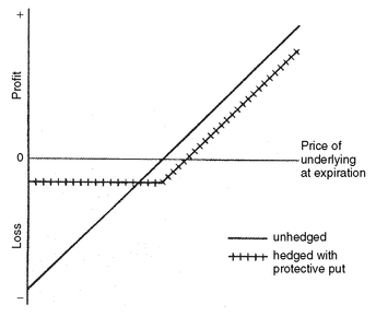
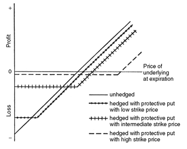
EXHIBIT 4 Protective Put Buying Strategy
EXHIBIT 5 Protective Put Buying Strategy with Different Strike Prices
2. Covered Call Writing Strategy Another options hedging strategy used by many portfolio managers is to sell calls against the bond portfolio. This hedging strategy is called a covered call writing strategy. The calls are usually out-of-the-money, and can be either calls on cash bonds or calls on interest rate futures. Covered call writing is just an outright long position combined with a short call position. Obviously, this strategy entails much more downside risk than buying a put to protect the value of the portfolio. In fact, many portfolio managers do not consider covered call writing a hedge.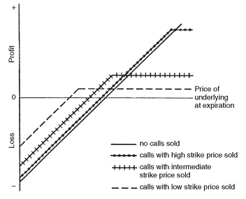
Regardless of how it is classified, it is important to recognize that while covered call writing has substantial downside risk, it has less downside risk than an unhedged long position alone. On the downside, the difference between the long position alone and the covered call writing strategy is the premium received for the calls that are sold. This premium acts as a cushion for downward movements in prices, reducing losses when rates rise. The cost of obtaining this cushion is the upside potential that is forfeited. When rates decline, the call option liability increases for the covered call writer. These incremental liabilities decrease the gains the manager would otherwise have realized on the portfolio in a declining rate environment. Thus, the covered call writer gives up some (or all) of the upside potential of the portfolio in return for a cushion on the downside. The more upside potential that is forfeited (that is, the lower the strike price on the calls), the more cushion there is on the downside. Exhibit 6 illustrates this point by comparing an unhedged position to several covered call writing strategies, each with a different strike price. Like the protective put buying strategy, there is no “right” strike price for the covered call writer.
EXHIBIT 6 Covered Call Writing Strategy with Different Strike Prices
3. Collar Strategy Another hedging strategy frequently used by portfolio managers combines protective put buying and covered call writing. By combining a long position in an out-of-the-money put and a short position in an out-of-the-money call, the manager creates a long position in a collar. Consequently, this hedging strategy is called a collar strategy. The manager who uses the collar eliminates part of the portfolio’s downside risk by giving up part of its upside potential. A long position hedged with a collar is shown in Exhibit 7.
The collar in some ways resembles the protective put, in some ways resembles covered call writing, and in some ways resembles an unhedged position. The collar is like the protective put buying strategy in that it limits the possible losses on the portfolio if interest rates go up. Like the covered call writing strategy, the portfolio’s upside potential is limited. Like an unhedged position, within the range defined by the strike prices the value of the portfolio varies with interest rates.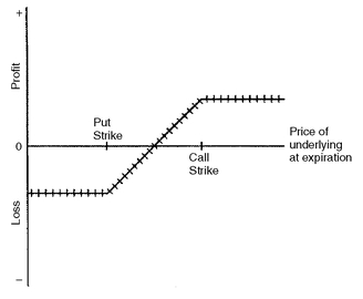
EXHIBIT 7 Long Position Hedged with a Collar
4. Selecting the “Best” Strategy Comparing the two basic strategies for hedging with options, one cannot say that the protective put buying strategy or the covered call writing strategy is necessarily the better or more correct options hedge. The best strategy (and the best strike price) depends upon the manager’s view of the market and risk tolerance. Paying the required premium to purchase a put is appropriate if the manager is fundamentally bearish. If, instead, the manager is neutral to mildly bearish, it is better to receive the premium by selling covered calls. If the manager prefers to take no view on the market at all, and to assume as little risk as possible, then the futures hedge is the most appropriate. If the manager is fundamentally bullish, then an unhedged position is probably the best strategy.
B. Steps in Options Hedging
Like hedging with futures (described in Section II), there are several steps that managers should consider before implementing their hedges. These steps include:
Step 1: Determine the option contract that is the best hedging vehicle. The best option contract to use depends upon several factors. These include option price, liquidity, and price correlation with the bond(s) to be hedged. Whenever there is a possibility that the option position may be closed out prior to expiration, liquidity is an important consideration. If a particular option is illiquid, closing out a position may be prohibitively expensive, so that the manager loses the flexibility to close out positions early, or rolling into other positions that may become more attractive. Correlation with the price of the underlying bond(s) to be hedged is another factor in selecting the right contract. The higher the correlation, the more precisely the final profit and loss can be defined as a function of the final level of rates. Low correlation leads to more uncertainty.
While most of the uncertainty in an options hedge usually comes from the uncertainty of interest rates, the correlation between the prices of the bonds to be hedged and the instruments underlying the options contracts determines the extent to which the hedging objective is accomplished. Low correlation leads to greater uncertainty.
Step 2: Find the appropriate strike price. For a cross hedge, the manager converts the strike price on the options that are bought or sold into an equivalent strike price for the bonds being hedged.
Step 3: Determine the number of contracts. The hedge ratio is the number of options to buy or sell.
Steps 2 and 3 can best be explained with examples using futures options.
C. Protective Put Buying Strategy Using Futures Options
As explained above, managers who want to hedge bond positions against a possible increase in interest rates find that buying puts on futures is one of the easiest ways to purchase protection against rising rates. To illustrate a protective put buying strategy, we can use the same FNMA bond that we used to demonstrate how to hedge with Treasury bond futures.353 In that example, a manager held $10 million par value of a 6.25% FNMA bond maturing 5/15/29 and used September 1999 Treasury bond futures to lock in a sale price for those bonds on the futures delivery date. Now we want to show how the manager could use futures options instead of futures to protect against rising rates.
On 6/24/99 the FNMA bond was selling for 88.39 to yield 7.20% and the CTD issue’s yield was 6.50%. For simplicity, it is assumed that the yield spread between the FNMA bond and the CTD issue remains at 70 basis points.
1. Selecting the Strike Price In our illustration, selecting the strike price means determining the minimum price that the manager wants to establish for the FNMA bonds. In our illustration we will assume that the minimum acceptable price (before the cost of the put options) is 84.453. This is equivalent to saying that the manager wants to establish a strike price for a put on the hedged bonds of 84.453. But, the manager is not buying a put on the FNMA bond. He is buying a put on a Treasury bond futures contract. Therefore, the manager must determine the strike price for a put on a Treasury bond futures contract that is equivalent to a strike price of 84.453 for the FNMA bond.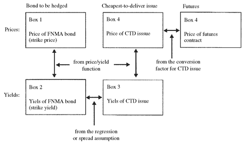
This can be done with the help of Exhibit 8. Notice that all the boxes are numbered and we shall refer to these numbered boxes as we illustrate the process. We begin at Box 1 of the exhibit. In our illustration, the portfolio manager set the strike price at 84.453 for the FNMA bond. Now we can calculate, given its coupon rate of 6.25%, its maturity, and the price of 84.453 (the strike price desired), that its yield is 7.573%. That is, setting a strike price of 84.453 for the FNMA bond is equivalent to setting a strike yield (or equivalently a maximum yield) of 7.573% in Box 2.
Now let’s move to Box 3—the yield of the cheapest-to-deliver issue. To move from Box 2 to Box 3 we use the assumption that the spread between the FNMA bond and the cheapest-to-deliver issue is a constant 70 basis points. Since the strike yield for the FNMA bond is 7.573%, subtracting 70 basis points gives 6.873% as the strike yield (or maximum yield) for the cheapest-to-deliver issue.
We again use the price/yield relationship to move from Box 3 to Box 4. The cheapest-to-deliver issue was the 11.25% of 2/15/15 issue. Given the maturity, the coupon rate, and the strike yield of 6.873%, the price is computed to be 141.136. This is the value that would go in Box 4.
Now for the final value we need—the strike price for the Treasury bond futures contract. We know that the converted price for any issue eligible for delivery on the bond futures contract is:
converted price = futures price × conversion factor
EXHIBIT 8 Calculating Equivalent Strike Prices and Yields for Hedging with Futures Options
In the case of the cheapest-to-deliver issue it is:
converted price for CTD issue = futures price × conversion factor for CTD issue
The goal is to get the strike price for the futures contract. Solving the above for the futures price we get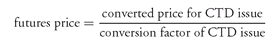
Since the converted price for the CTD issue in Box 4 is 141.136 and the conversion factor is 1.283, the strike price for the Treasury bond futures contract is: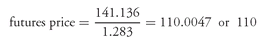
A strike price of 110 for a put option on a Treasury bond futures contract is roughly equivalent to a put option on our FNMA bond with a strike price of 84.453.
The foregoing steps are always necessary to obtain the appropriate strike price on a futures put option. The process is not complicated. It simply involves (1) the relationship between price and yield, (2) the assumed relationship between the yield spread between the bonds to be hedged and the cheapest-to-deliver issue, and (3) the conversion factor for the cheapest-to-deliver issue. Once again, the success of the hedging strategy will depend on (1) whether the cheapest-to-deliver issue changes and (2) the yield spread between the bonds to be hedged and the cheapest-to-deliver issue.
2. Calculating the Number of Options Contracts Since we assume a constant yield spread between the bond to be hedged and the cheapest-to-deliver issue, the hedge ratio is determined using the following equation, which is similar to equation (7): 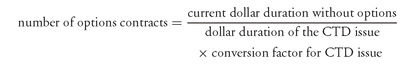
The current duration refers to the duration at the time the hedge is placed. Recall that the dollar durations are calculated as of the date that the hedge is expected to be removed using the target yield for the bond to be hedged. For the protective put buying strategy, we will assume that the hedge will be removed on the expiration date of the option (assumed to be the end of September 1999). To obtain the current dollar duration for the bond, the target yield is the 7.573% strike yield of the FNMA bond. The current dollar duration for the FNMA bond as of the end of September 1999 for a 50 basis point change in rates and for a target yield of 7.573% would produce a value of $512,320. This value differs from the current dollar duration used to compute the number of contracts when hedging with futures. That value was $545,300 because it was based on a target yield of 7.26%.
The dollar duration for the CTD issue is based on a different target price (i.e., the minimum price) than in the hedging strategy with futures. The target price in the futures hedging strategy was 113 and the dollar duration of the CTD issue was $6,255. For the protective put buying strategy, since the strike price of the futures option is 110 (the target price in this strategy), it can be shown that the dollar duration for the CTD issue for a 50 basis point change in rates is $6,021.
Therefore, we know that for a 50 basis point change in rates: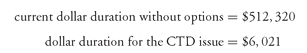
Substituting these values and the conversion factor for the CTD issue of 1.283 into the formula for the number of options contracts, we find that: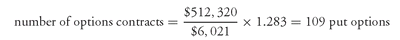
Thus, to hedge the FNMA bond position with put options on Treasury bond futures, 109 put options must be purchased.
3. Outcome of the Hedge To create a table for the protective put hedge, we can use data from Exhibit 2. Exhibit 9 shows the scenario analysis for the protective put buying strategy. The first five columns are the same as in Exhibit 2. For the put option hedge, Column (6) shows that the value of the put position at expiration equals zero if the futures price is greater than or equal to the strike price of 110. If the futures price is below 110, then the options expire in the money and:
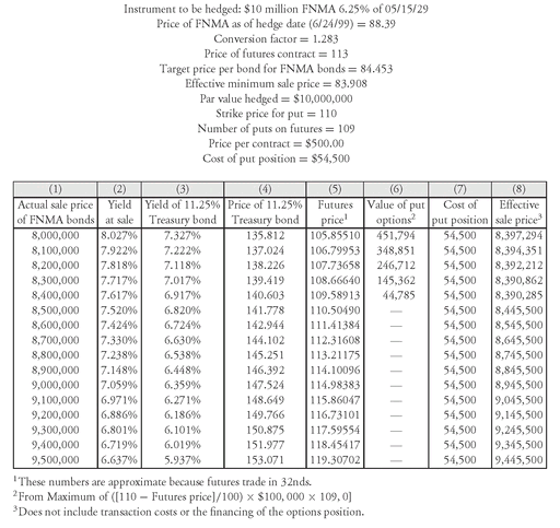
value of put option position = ([110 - futures price]/100) × $100, 000
× number of put options
× number of put options
For example, for the first scenario in Exhibit 9, the corresponding futures price is 105.8551 and the value of the put options is
([110 - futures price]/100) × $100, 000 × 109 = $451, 794
EXHIBIT 9 Hedging a Nondeliverable Bond to a Delivery Date with Puts on Futures
The effective sale price for the FNMA bonds is then equal to
effective sale price = actual sale price + value of put option position - option cost
Let’s look at the option cost. Suppose that the price of the put option with a strike price of 110 is $500 per contract. The cost of the protection is $54,500 (109 × $500, not including financing costs and commissions). This cost is shown in Column (7) and is equivalent to $0.545 per $100 par value hedged.
The effective sale price for the FNMA bonds in each scenario, shown in the last column of Exhibit 9, is never less than 83.902. This equals the price of the FNMA bonds equivalent to the futures strike price of 110 (i.e., 84.453), minus the cost of the puts (that is, $0.545 per $100 par value hedged). This minimum effective price is something that can be calculated before the hedge is initiated. (As prices decline, the effective sale price actually exceeds the target minimum sale price of 83.908 by a small amount. This is due only to rounding; the hedge ratio is left unaltered although the relative dollar durations used in the hedge ratio calculation change as yields change.) As prices increase, however, the effective sale price of the hedged bonds increases as well; unlike the futures hedge shown in Exhibit 2, the options hedge protects the investor if rates rise, but allows the investor to profit if rates fall.
D. Covered Call Writing Strategy with Futures Options
Unlike the protective put buying strategy, the purpose of covered call writing is not to protect a portfolio against rising rates. The covered call writer, believing that the market will not trade much higher or much lower than its present level, sells out-of-the-money calls against an existing bond portfolio. The sale of the calls brings in premium income that provides partial protection in case rates increase. The premium received does not, of course, provide the kind of protection that a long put position provides, but it does provide some additional income that can be used to offset declining prices. If, instead, rates fall, portfolio appreciation is limited because the short call position constitutes a liability for the seller, and this liability increases as rates decline. Consequently, there is limited upside price potential for the covered call writer. Of course, this is not a concern if prices are essentially going nowhere; the added income from the sale of call options is obtained without sacrificing any gains.
To see how covered call writing with futures options works for the bond used in the protective put example, we construct a table much as we did before. We assume in this illustration that a sale of a call option with a strike price of 117 is selected by the manager.354 As in the futures hedging and protective buying strategies it is assumed that the hedged bond will remain at a 70 basis point spread over the CTD issue. We also assume that the price of each call option is $500.
Working backwards from box 5 in Exhibit 8, a strike price for the futures option of 117 would be equivalent to the following at the expiration date of the call option: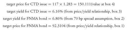
Given the above information, the current dollar duration for the FNMA bond and the dollar duration of the CTD issue can be computed. The information above represents values as of the expiration date of the call option. It can be shown that the dollar durations based on a 50 basis point change in rates are: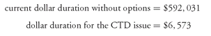
Substituting these values and the conversion factor for the CTD issue of 1.283 into the formula for the number of options contracts, we find: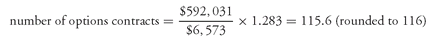
The proceeds received from the sale of 116 call options are $58,000 (116 calls × $500) and proceeds per $100 of par value hedged are $0.580.
While the target price for the FNMA bond is 92.3104, the maximum effective sale price is determined by adjusting the target price by the proceeds received from the sale of the call options. The maximum effective sale price is 92.8904 (= 92.3104 + 0.5800).
Exhibit 10 shows the outcomes of the covered call writing strategy. The first five columns of the exhibit are the same as Exhibit 9. In Column (6), the liability resulting from the call option position is shown. The liability is zero if the futures price is less than the strike price of 117. If the futures price for the scenario is greater than 117, the liability is calculated as follows:
([futures price - 117]/100) × $100, 000 × number of call options
For example, consider a sale price for the FNMA bond of $9.5 million. The corresponding futures price is 119.30702. The number of call options sold is 116. Therefore,
That is, ([119.30702 - 117]/100) × $100, 000 × 116 = $267,614
That is,
effective sale price = actual sale price + proceeds from sale of the call options
- liability of call positiona
- liability of call positiona
EXHIBIT 10 Writing Calls on Futures against a Nondeliverable Bond
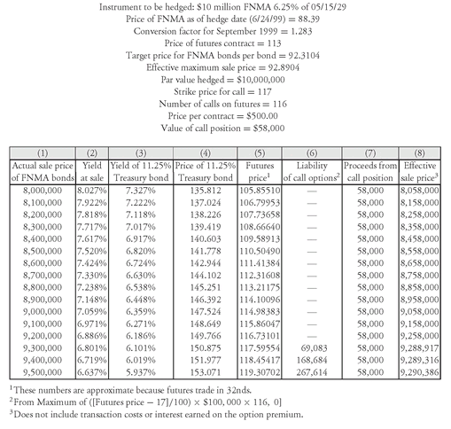
Since the proceeds from sale of the call options is $58,000, then
effective sale price = actual sale price + $58,000 - liability of call position
The last column of Exhibit 10 shows the effective sale price for each scenario.
As Exhibit 10 shows, if the hedged bond trades at 70 basis points over the CTD issue as assumed, the maximum effective sale price for the hedged bond is, in fact, slightly over 92.8904. The discrepancies shown in the exhibit are due to rounding.
E. Comparing Alternative Strategies
In this chapter we reviewed three basic strategies for hedging a bond position: (1) hedging with futures, (2) hedging with out-of-the-money puts, and (3) covered call writing with out-of-the-money calls. Similar, but opposite, strategies exist for managers who are concerned that rates will decrease. As might be expected, there is no “best” strategy. Each strategy has advantages and disadvantages, and we never get something for nothing. To get anything of value, something else of value must be forfeited.
To make a choice among strategies, it helps to compare the alternatives side by side. Using the futures example from Section II B and the futures options examples from Section IV C, Exhibit 11 shows the final values of the portfolio for the various hedging alternatives. It is easy to see that no one strategy dominates the others in every scenario.
Consequently, we cannot conclude that one strategy is the best strategy. The manager who makes the strategy decision makes a choice among probability distributions, not usually among specific outcomes. Except for the perfect hedge, there is always some range of possible final values of the portfolio. Of course, exactly what that range is, and the probabilities associated with each possible outcome, is a matter of opinion.
EXHIBIT 11 Comparison of Alternative Strategies
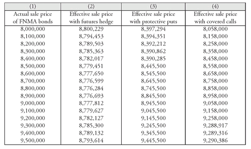
F. Hedging with Options on Cash Instruments
Hedging a position with options on cash bonds is relatively straightforward. Most strategies, including the purchase of protective puts, covered call writing, and buying collars, are essentially the same whether futures options or options on physicals are used. As explained, an option on a physical is an option on a bond. In our illustrations we used options on futures because they are the more actively traded types of futures contracts and therefore the contracts used in hedging. While there are mechanical differences in the way the two types of option contracts are traded, the basic economics of the hedging strategies are virtually identical.
Using options on physicals frequently eliminates much of the basis risk associated with a futures options hedge. For example, a manager of Treasury bonds or notes can usually buy or sell options on the exact security held in the portfolio. Using options on futures, rather than options on Treasury bonds, introduces additional elements of uncertainty.
Given the illustration presented above, and given that the risk-return profile of options on physicals and options on futures are essentially identical, additional illustrations for options on physicals are unnecessary. The only important differences are the calculations of the hedge ratio and the equivalent strike price. To derive the hedge ratio, we always resort to an expression of relative dollar durations. Thus, assuming a constant spread, the hedge ratio for options on physicals is: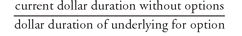
If a relationship is estimated between the yield on the bonds to be hedged and the instrument underlying the option, the appropriate hedge ratio is: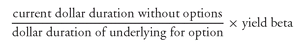
Unlike futures options, there is only one deliverable, so there is no conversion factor. When cross hedging with options on physicals, the procedure for finding the equivalent strike price on the bonds to be hedged is similar. Given the strike price of the option, the strike yield is determined using the price/yield relationship for the instrument underlying the option. Then given the projected relationship between the yield on the instrument underlying the option and the yield on the bonds to be hedged, an equivalent strike yield is derived for the bonds to be hedged. Finally, using the yield-to-price formula for the bonds to be hedged, the equivalent strike price for the bonds to be hedged can be found.
V. USING CAPS AND FLOORS
Interest rate caps can be used in liability management to create a cap for funding costs. Combining a cap and a floor creates a collar for funding costs. Floors can be used by buyers of floating-rate instruments to set a floor on the periodic interest earned. To reduce the cost of a floor, a manager can sell a cap. By doing so, the manager limits the upside on the coupon rate of a floating-rate instrument should rates rise, thereby creating a collar for the coupon rate.
To see how interest rate caps and floors can be used for asset/liability management, consider the problems faced by the commercial bank and the life insurance company discussed in Section III A. Recall that the bank’s objective is to lock in a spread over its cost of funds. Yet because the bank borrows short term, its cost of funds is uncertain. The bank may be able to purchase a cap, however, so that the cap rate plus the cost of purchasing the cap is less than the rate it is earning on its fixed-rate commercial loans. If short-term rates decline, the bank does not benefit from the cap, but its cost of funds declines. The cap therefore allows the bank to impose a ceiling on its cost of funds while retaining the opportunity to benefit from a decline in rates.
The bank can reduce the cost of purchasing the cap by selling a floor. In this case, the bank agrees to pay the buyer of the floor if the reference rate falls below the strike rate. The bank receives a fee for selling the floor, but it has sold off its opportunity to benefit from a decline in rates below the strike rate. By buying a cap and selling a floor, the bank has created a predetermined range for its cost of funds (i.e., a collar).
Recall the problem of the life insurance company that guarantees an 8% rate on a GIC for four years and is considering the purchase of a floating-rate instrument in a private placement transaction. The risk the company faces is that interest rates will fall so that it will not earn enough to realize the 8% guaranteed rate plus a spread. The life insurance company may be able to purchase a floor to set a lower bound on its investment return, yet retain the opportunity to benefit should rates increase. To reduce the cost of purchasing the floor, the life insurance company can sell an interest rate cap. By doing so, however, it forfeits the opportunity to benefit from an increase in the reference rate above the strike rate of the cap.
..................Content has been hidden....................
You can't read the all page of ebook, please click here login for view all page.