Chapter 7. Laplace’s Equation, Irrotational and Porous-Media Flows
7.1. Introduction
The previous chapter dealt with fluid motions in which the viscosity always played a key role. However, away from a solid boundary, the effect of viscosity is frequently small and may be neglected. The example was given at the end of Section 5.2 of the rotation of a cup containing coffee, in which there was little perceptible rotation of the liquid itself. For a cup of molasses, the situation would obviously be different.
There are several practical situations, in which the fluid can be treated as essentially inviscid, occurring for example in the flow of air relative to an airplane, flow of water in lakes and harbors, surface waves on water, air motion in tornadoes, etc., and these will be discussed in this chapter. It is understood that we are not inquiring about the motion in either of the following two cases:
1. Very close to a solid boundary, where the action of viscosity is important, and which will be discussed in Chapter 8.
2. In the wake of a solid obstacle, where laminar instabilities or turbulence can occur at high Reynolds numbers—for illustrations see the applications of computational fluid dynamics using COMSOL and FlowLab in Examples 9.4 (flow through an orifice plate) and 13.4 (flow in the wake of a cylinder).
Section 7.3 will demonstrate that these inviscid flows are governed by Laplace’s equation. Somewhat paradoxically, Section 7.9 will show that Laplace’s equation also applies to a phenomenon that is apparently at the other end of the spectrum—to the flow of viscous fluids in porous media, which is of considerable practical significance in the production of oil, the underground storage of natural gas, and the flow of groundwater. And, as will be seen in Chapter 10, Laplace’s equation plays an important role in the rise velocity of large bubbles in liquids and fluidized beds, and also governs the pressure distribution in the particulate phase of fluidized beds. Finally, Example 12.3 shows that potential-flow theory can be applied to electroosmotic flow around a particle in a microchannel.
Motion of an inviscid fluid. We start by rederiving Bernoulli’s equation for inviscid fluids, but this time in any number of space dimensions. In such cases, with μ = 0, Eqn. (5.68) yields for the usual case of an incompressible fluid the so-called Euler equation:
in which the body force vector F is typically the gradient of a scalar Φ (known as the body-force potential):
where gravity is assumed to be the body force and z is oriented vertically upwards. Since ρ is constant, Eqns. (7.1) and (7.2) yield:
The following vector identity is quoted without proof:

in which v2 = v · v, and Eqn. (5.30) has already shown the vorticity ζ to equal:

where ω is the angular velocity of the fluid at a point.
Hence, from Eqns. (7.3) and (7.4),

which, for steady flow, reduces to
That is, the vector v × ζ is normal to the surfaces
where c is a constant for a particular surface, which must therefore contain v (that is, streamlines) and ζ (vortex lines). The tangent to a streamline has the direction of the velocity; that to a vortex line has the direction of vorticity. For irrotational flows, which have zero vorticity (ζ = 0), the constant c is the same throughout the fluid, giving Bernoulli’s equation, of considerable importance for the motion of ideal frictionless fluids.
Another special case of Eqn. (7.5) occurs for transient irrotational flows:
which finds application in the study of surface waves in Section 7.11.
7.2. Rotational and Irrotational Flows
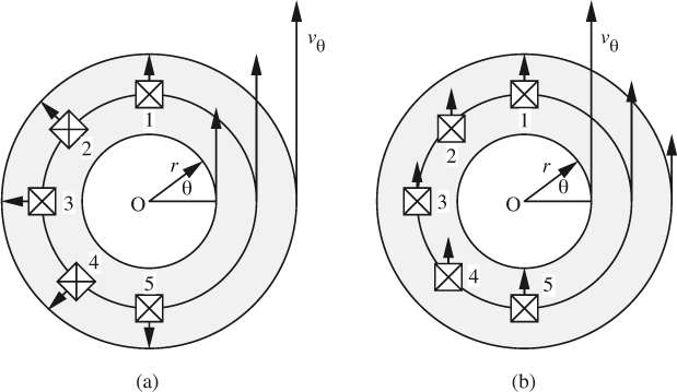
Fig. 7.1 shows examples of both irrotational and rotational flows, in each of which the streamlines, viewed here from above the free surface of the liquid in a container, are concentric circles. To visualize the flows, a cork is floating in the liquid, and is here designated as a square with (for easy visualization) diagonals and a protruding arrow. Although both flows consist of a vortex, in which fluid particles are following circular paths, the two cases are quite different:
(a) The first case corresponds to a forced vortex in which (mainly due to a rotating container and the action of viscosity) the liquid is turning with a constant angular velocity ω, just as if it were a solid body. Thus, the sole velocity component is given by υθ = rω, which increases with radius. As the path 1– 2–3–4–5 is followed, the cork clearly rotates counterclockwise, thus indicating a counterclockwise angular velocity throughout. The flow is therefore rotational.
(b) The second case corresponds to a free vortex, which can occur in essentially inviscid liquids, the sole velocity component now being inversely proportional to the radius; that is, υθ = c/r. As the path 1–2–3–4–5 is followed, the cork maintains its orientation, indicating that the vorticity is zero. The flow is therefore irrotational.
The cyclone separator, discussed in Section 4.8, presents an example of a free vortex in the central core of the equipment; however, in a small region near the entrance of the separator, the flow approximates a forced vortex, because of the driving effect of the inlet gas. The draining of a bathtub or sink offers another example of a free vortex, since the velocity in the angular direction speeds up as the drain hole is approached. The question of the direction of rotation into the drain has been nicely answered by Cope.1
1 Yes, it is true that—if the water is perfectly still before the drain plug is pulled—the direction of rotation of the bathtub vortex does depend on whether it is in the northern or southern hemisphere. However, any quite small initial rotation of the water would dominate this natural effect caused by the earth’s rotation. In a letter to the editor of the American Scientist, Vol. 71 (Nov/Dec 1983), Winston Cope stated: “I spent most of 1974 with the U.S. Navy at the South Pole, where one of my projects was to demonstrate the Coriolis effect. At the poles the Coriolis effect is greatest, and we used a smaller tank than described by Dr. Sibulkin: half of a 50-gallon drum. Because the temperature of the room was below freezing for water, a solution of ethylene glycol was used. It took 3–5 days for the rotation effects due to filling to subside, but a small, consistently clockwise vortex resulted as the fluid drained. The motion was easily detected by means of talc particles on the surface. The rotation of the vortex was the same whether the fluid drained through a nozzle toward the floor, or from a nozzle through a siphon from above.”
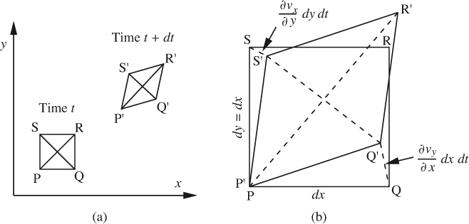
Vorticity and angular velocity. We have already seen that the angular velocity at a point is one-half of the vorticity, giving (in two dimensions):
which will now be interpreted and verified for two-dimensional flow.
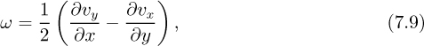
Consider the situation in Fig. 7.2(a), in which, over a small time step dt, an initially square fluid element PQRS moves to a new location P′Q′R′S′. Observe that the element translates (moves), deforms, and possibly rotates, as discussed earlier following Fig. 5.15. Fig. 7.2(b) shows both elements enlarged and superimposed to have a common lower left-hand corner, with P and P′ coincident. The angular velocity of the element is determined by finding out how much the diagonal PR has rotated when it assumes its new position P′R′. Observe that PQ has rotated counterclockwise to its new position P′Q′. The y velocity υy of Q exceeds that of P by an amount (∂υy/∂x) dx; thus, in a time dt, the distance QQ′ will be (∂υy/∂x) dx dt.
The angle Q′PQ is therefore (∂υy/∂x) dt, so that the (counterclockwise) angular velocity of PQ is ∂υy/∂x. By a similar argument, the clockwise angular velocity of PS is ∂υx/∂y.
The counterclockwise angular velocity of the diagonal PR is the mean of the angular velocities of PQ and PS:
A comparison with the z component of vorticity given in Eqn. (5.29):
reveals again that the angular velocity is one-half of the vorticity.
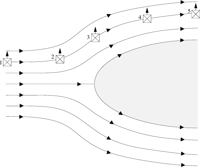
An additional example of irrotational flow, viewed from above a free surface, is given in Fig. 7.3, for liquid motion past a blunt-nosed solid. Again, the floating cork maintains a constant orientation. Observe in our idealization that the fluid in contact with the solid object violates the “no-slip” boundary condition, and is allowed to have a finite velocity, because there are no viscous stresses to retard it. In practice, of course, the velocity at the boundary would be zero, but would quickly build up to the value in the “mainstream” across a very thin boundary layer. Thus, apart from this boundary layer, the irrotational flow solution can still give a fairly accurate picture of the overall flow.
Example 7.1—Forced and Free Vortices
The flow pattern in a liquid stirred in a large closed cylindrical tank can be approximated by a forced vortex of radius a and angular velocity ω (corresponding to the location of the stirrer), surrounded by a free vortex that extends indefinitely radially outward, as shown in Fig. E7.1.1.

If the pressure is p∞ for large values of r, derive and plot expressions for the tangential velocity υθ and pressure p as functions of radial location r. If the top of the tank is removed, so that the liquid is allowed to have a free surface, comment on its shape. Also, discuss how the free vortex is generated in this example.
Solution
First, consider the tangential velocity υθ in the two regions:
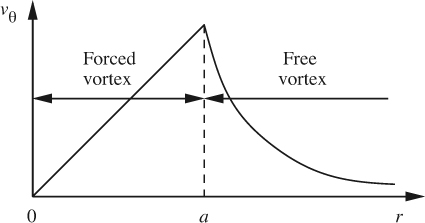
At the junction between the two regions, where r = a, the velocities must be identical, so that (υθ)r=a = aω = c/a; thus, the constant is c = ωa2 and the velocities in the two regions are:
representative profiles being shown in Fig. E7.1.2.
Second, since there is zero vorticity in the free vortex, Bernoulli’s equation applies, it being noted that the velocity declines to zero for large r:

so that the pressure at the junction between the two vortices is:
For the forced vortex, the radial variation of pressure is already given in Eqn. (1.44):
a result that can also be obtained from the full r momentum balance in cylindrical coordinates, Eqn. (5.75), by making appropriate simplifications and substituting υθ = rω. Integration of Eqn. (E7.1.5), noting that p = pa at r = a, gives:

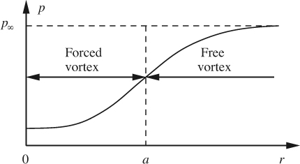
A representative complete pressure distribution is given in Fig. E7.1.3. Note that the overall pressure changes in the two vortices are identical (ρω2a2/2). If the liquid has a free surface, the pressure toward the bottom of its container must be balanced hydrostatically by a column of liquid that extends to the free surface. Thus, the free surface must have a shape that resembles the curve in Fig. E7.1.3, and this is substantiated by experiment.
Regarding the generation of the free vortex, consider the liquid in the region r > a to be initially at rest when the stirrer is turned on. With appropriate simplifications, the θ momentum balance becomes:
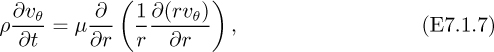
and will govern how υθ builds up to its final value as shown in Fig. E7.1.2, at which stage the right-hand side of Eqn. (E7.1.7) is zero. Somewhat paradoxically in this example, viscosity is important in determining the final velocity profile, even though the resulting free vortex region has zero vorticity.
7.3. Steady Two-Dimensional Irrotational Flow
Rectangular Cartesian coordinates. Most of the development in this section will be in terms of x/y coordinates, after which the important relationships will be restated for two-dimensional cylindrical coordinates.
For inviscid fluids, Bernoulli’s equation, (7.7), is already available for relating changes in pressure, velocity, and elevation. Here, we use the continuity equation,
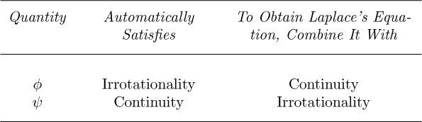
and the irrotationality condition to show that the flow can be represented by a velocity potential φ that obeys Laplace’s equation.
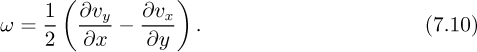
Note first that the angular velocity of a fluid element is caused by shear stresses, which act tangentially to the surface of the element, and may have a net resulting moment about its center of gravity, thus causing it to rotate. (Pressure forces act normal to the surface of an element, and have no resulting moment, so cannot induce rotation of the element.) In the absence of viscosity, there can be no shear stresses. Hence, an element of fluid starting with zero angular velocity cannot acquire any. Therefore, from Eqn. (7.10), zero angular velocity implies that:
Velocity potential. Now consider a new function, the velocity potential φ, which is such that the velocity components υx and υy are obtained by differentiation of φ in the x and y directions:
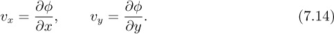
That is, the vector velocity is the gradient of the velocity potential2:
2 Some writers define the potential with a negative sign: v = –∇φ. The reader should therefore be alert as to which convention is being used.
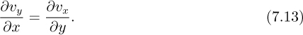
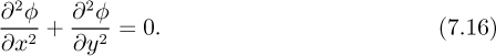
The reader can check that the concept of the velocity potential automatically satisfies the irrotationality condition, Eqn. (7.13). Substitution of the velocity components from Eqn. (7.14) into the continuity equation, (7.12), gives Laplace’s equation for the velocity potential:
Stream function. As an alternative, we can define a stream function, ψ, such that the velocity components υx and υy are obtained by differentiation of ψ in the y and –x directions, respectively:
Compared with Eqn. (7.14), note the reversed order of x and y, and also the minus sign in the expression for υy.
The reader can also check that the concept of the stream function automatically satisfies the continuity equation, (7.12). Substitution of the velocity components from Eqn. (7.17) into the irrotationality condition, (7.13), gives Laplace’s equation for the stream function in two-dimensional irrotational flows:
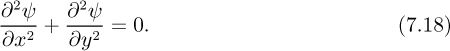
Table 7.1 summarizes the above facts about the velocity potential and the stream function. It will also be shown in the next section that a contour of constant ψ represents the path followed by the fluid.
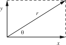
Two-dimensional cylindrical coordinates. First, examine the more commonly occurring case for which υz = 0. For r/θ coordinates—shown in relation to x/y coordinates in Fig. 7.4—the corresponding relationships between the velocity components and the potential and stream function can be proved:
From Eqn. (5.49) and Table 5.4, the continuity equation and irrotationality condition are:
Appropriate substitutions again lead to Laplace’s equation in the potential function and stream function:

Second, note that two-dimensional flows may also exist in cylindrical coordinates with υθ = 0, in which υr and υz are the velocity components of interest. In this case, the appropriate relations for the velocities, potential function, and stream function are:
Note that the second-order equation for the stream function is no longer Laplace’s equation.
Flow in porous media. The treatment in Section 7.9 will show that the pressure for the flow of a viscous fluid, such as oil, in a porous medium, such as a permeable rock formation, also obeys Laplace’s equation (in two-dimensional rectangular coordinates, for example):
Thus, much of the discussion in this chapter applies not only to flow of essentially inviscid fluids, but also to the flow of viscous fluids in porous media. Obvious important applications are to the recovery of oil from underground rock formations, to the motion of groundwater in soil, and the underground storage of natural gas. A representative example appears in Section 7.9.
7.4. Physical Interpretation of the Stream Function
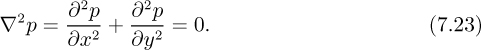
For steady two-dimensional flow in x/y coordinates, an alternative and equivalent definition to that of Eqn. (7.17) for the stream function is given by reference to Fig. 7.5(a), in which a family of streamlines (lines of constant ψ) is shown. Consider the flow rate Q, per unit depth normal to the plane of the diagram, between streamlines that have values of the stream function equal to ψ1 and ψ2.
Fig. 7.5 (a) Flow rate Q crossing paths PS and PT joining streamlines with values ψ1 and ψ2; (b) velocity components υx and υy crossing segments dy and dx between neighboring streamlines.
The equivalent viewpoint to that of Eqn. (7.17) is to define the flow rate Q as the difference between the two values of the stream function, namely, Q = ψ2 –ψ1. The sign convention is such that Q is taken to be positive if flowing from left to right across a path such as PS from ψ1 to ψ2. That is, if the flow is physically in the indicated direction, then ψ2 > ψ1; if it is in the opposite direction, then ψ2 <ψ1.
Since the value of ψ is constant along a streamline, the flow rate Q will still be the same across any other path such as PT. It immediately follows that the flow across ST is zero, and that no flow can occur across a streamline; hence, the flow is always in the direction of the streamline passing through any point. Representative units for Q and ψ are m2/s.
To verify that this viewpoint is completely consistent with that of Eqn. (7.17), consider Fig. 7.5(b), which shows three points, P, A, and B, on three streamlines that are only differentially separated. Across PB and PA, paying attention to the direction of flow as defined above, the flow rates dQx and dQy per unit depth are:
Thus, from Eqn. (7.24), the velocity components are identical with those given previously:
Since we have already established that the direction of the flow is normal to the equipotentials, the streamlines and equipotentials must everywhere be orthogonal to one another, and a representative situation is shown in Fig. 7.6.
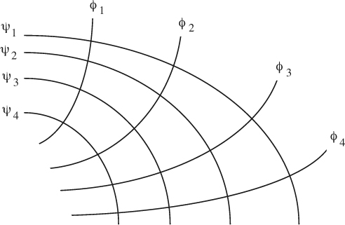
The reader should consider the direction of flow if the values of the stream function ψ1 ...ψ4 are in ascending or descending order, and similarly for the values of the equipotentials φ1 ...φ4.
7.5. Examples of Planar Irrotational Flow
Here, we examine a few two-dimensional irrotational flows, in which it is necessary to become accustomed to working in either rectangular (x/y) or cylindrical (r/θ) coordinates, depending on the problem at hand.
Uniform stream. One of the simplest flows is that in which the two velocity components are υx = U (a specified value) and υy = 0, corresponding to a uniform stream in the x direction, as shown in Fig. 7.7. The reader can check that the velocity potential and stream function are given by:

Observe also that if the function for either φ or ψ is known, then the other one can usually be readily deduced. For example, suppose that φ is given from Eqn. (7.25). By using the definitions of Eqn. (7.14), the x and y velocity components can be obtained and then equated to the corresponding derivatives of the stream function from Eqn. (7.17):
Integration of the two relations in Eqn. (7.27) gives two expressions for the stream function:
in which f(x) and g(y) are arbitrary functions of integration. (Remember, we are integrating partial differential equations, not ordinary differential equations, and therefore obtain functions of integration, not just constants of integration.) However, the only way the two expressions for ψ in Eqn. (7.28) can be mutually consistent is if f(x) = c and g(y) = Uy + c, in which c is a constant, conveniently—but not necessarily—taken as zero. Therefore, we conclude that ψ = Uy, in agreement with the stated function in Eqn. (7.26).
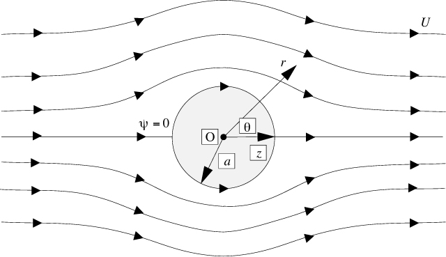
Flow past a cylinder. Fig. 7.8 illustrates the steady flow of an inviscid fluid past a cylinder of radius a; far away from the cylinder, the velocity is U in the x direction and zero in the y direction. In this particular situation, it is convenient to introduce polar coordinates, r and θ, in addition to x and y, such that:
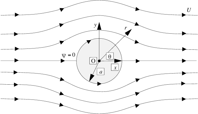
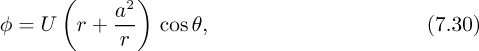
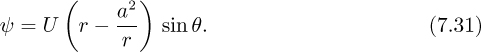
The velocity potential and stream function are:
These functions are verified if they satisfy the following three conditions:
1. Laplace’s equations. It will be left as an exercise to prove compatibility with Eqn. (7.21):

2. Uniform x velocity far away from the cylinder. As the radial coordinate becomes large (r → ∞), the potential and stream function become:
which are readily shown to be consistent with υx = U and υy = 0 far away from the cylinder.
3. Zero radial velocity at the surface of the cylinder. Because in our idealization there is no viscosity, no boundary layer forms on the surface of the cylinder, and this surface is itself a streamline—more correctly, a divided streamline, since there is flow around both sides of the cylinder. It therefore follows that there can be no radial component of the velocity at r = a. For the velocity potential and stream function, we have:


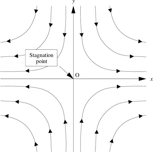
Investigate the potential flow whose stream function in x/y coordinates is:
Solution
From Eqn. (7.17), the two velocity components are:
leading to the following observations (c is assumed to be positive):
1. Along the x-axis (y = 0), υy = 0, and the flow is parallel to the x-axis. For positive values of x, the flow is to the right, and for negative values of x, it is to the left.
2. Along the y-axis (x = 0), υx = 0, and the flow is parallel to the y-axis. For positive values of y, the flow is downward, and for negative values of y, it is upwards.
3. The equation for the stream function, ψ = cxy, is that of a family of hyperbolas.
4. There is a stagnation point at the origin, O.
With above in mind, it is now possible to deduce the flow pattern, which is shown in Fig. E7.2.1. It could occur when two streams—one coming from the +y direction and the other coming from the –y direction—meet each other. Observe that the streams are deflected so that they leave in the +x and –x directions.
However, there are other possibilities. We could simply choose to ignore the lower half of the region, for negative values of y. In this case, the flow would essentially be that of a downward wind against a horizontal plane, such as the ground. We could also focus exclusively on the upper right-hand quadrant, for example, in which case the flow would be that in a corner.
The derivation of the corresponding velocity potential is left as an exercise.
Line source. Fig. 7.9(a) shows a “line” source that extends indefinitely along an axis of symmetry, from which it emits a flow uniformly in all radial directions. The strength m of the source is defined such that the total volumetric flow rate emitted by unit length of the source is 2πm. (The inclusion of the factor 2π is merely a convenience, since it simplifies the subsequent equations.)
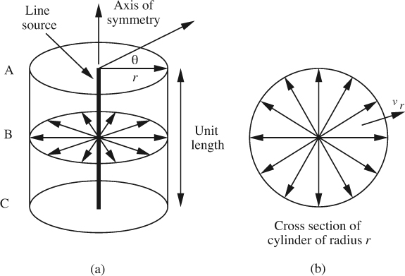
A view along the axis of a circular section of radius r at any location—such as at B—is shown in Fig. 7.9(b). If the outwards radial velocity is υr, the total volumetric flow rate per unit depth is the velocity υr times the surface area 2πr of the imaginary cylindrical shell through which the flow is passing:
Since there is no swirl, note that υθ = 0. Thus, the potential and stream functions corresponding to the line source are, apart from a possible constant:
A line source is a useful “building block” in constructing two-dimensional flow patterns, as will be seen in Example 7.3. A line source of negative strength is called a line sink, and resembles a vertical well into which a liquid such as oil or water is flowing from the surrounding earth or porous rock.
Example 7.3—Combination of a Uniform Stream and a Line Sink (C)
An inviscid fluid flows with velocity U parallel to a wall, as shown in Fig. E7.3.1. The narrow slot S is long in the direction normal to the diagram, and a volumetric flow rate Q per unit slot length is withdrawn. (The particle shown at x = X is not needed in this example, but will be important in Problem 7.13.)

Derive an expression for the stream function, and sketch several representative streamlines. At a large value of y, what is the value of x for the dividing streamline? Discuss a practical application of this type of flow.
Solution
The overall stream function is the sum of the stream functions for the following two flows:
1. A uniform stream in the direction of the negative y axis. By analogy with Eqn. (7.26):
2. Because the slot is narrow, it is essentially a line sink with its axis normal to the plane of the diagram. Since a flow rate Q per unit depth is withdrawn from just half the total plane, it would be 2Q for the entire plane of Fig. 7.9(b). Therefore, the corresponding source strength for use in conjunction with Eqn. (7.39) is m = –Q/π, giving the following stream function for the slot:
The stream function for the combination of uniform stream and line sink is:
Representative streamlines are shown in Fig. E7.3.2. Note that the width of the incoming stream that is diverted through the slot is Q/U—this value, when multiplied by the velocity U, gives the required slot flow rate Q.
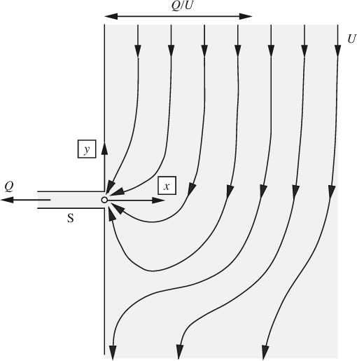
The flow is important because it corresponds approximately to the diversion of part of a large river into a small side channel, or of a gas into a sampling port. And—if the direction of Q were reversed—the flow would be that of a small tributary into a river.
Example 7.4—Flow Patterns in a Lake (COMSOL)
Fig. E7.4.1 shows a bird’s-eye view of a lake whose shape is approximated by merging two ellipses and two rectangles. These rectangles protrude to the “west” at AB and to the “south” at CD, and can serve as an inlet and an exit to and from the lake, respectively.
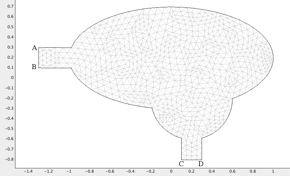
Fig. E7.4.1 A bird’s-eye view of a lake, which results from merging two ellipses and two rectangles. The finite-element mesh has been refined once.
Note that the inviscid flow (possibly with rotation) is governed by Poisson’s equation:

in which ψ is the stream function. In COMSOL, Eqn. (E7.4.1) is represented as –∇ · (c∇u) = f, with c = 1.
For two-dimensional flow, it can readily be shown that –∇2ψ = ζ, where ζ = (∂υy/∂x – ∂υx/∂y) is the vorticity, so that f acts as a source term for the vorticity. If f = 0, the vorticity will be zero and there will be no rotation. But a positive value of f would mean that the vorticity is positive, corresponding to a counterclockwise rotation. And a negative value of f would indicate a clockwise rotation. Such rotations could result from the shear stresses induced on the surface of the lake by a nonuniform wind, whose velocity υy varies with x as shown in Fig. E7.4.2. Note that in the eastern region (x > 0) the intensity increases toward the east, and in the western region (x < 0) the intensity increases toward the west.
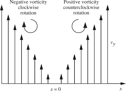
Fig. E7.4.2 Velocities υy corresponding to a nonuniform wind, shearing the surface of the water in the lake and generating vorticity as indicated.
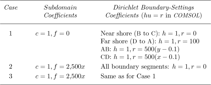
Solve for the pattern of streamlines for each of the following three cases:
1. The stream function equals ψ = 0 along the near shore between points B and C and equals ψ = 100 along the far shore between points D and A. From B to A and from C to D, ψ varies linearly from zero to 100. Everywhere, f = 0.
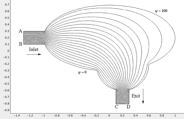
2. The rivers are “turned off,” so the lake is now isolated and its boundary becomes the single streamline ψ = 0. However, the vorticity source term is now f = 2,500 x. Thus, we would expect a counterclockwise rotation for x> 0 and a clockwise rotation for x< 0.
3. Finally, consider the case of both river flow and the nonuniform wind. The boundary conditions will be the same as for Case 1, but the expression for f will be the same as for Case 2.
Solution
1. In COMSOL, choose the sequence New, PDE Modes, Classical PDEs, and Poisson’s Equation.
2. After the sequence Options, Axes/Grid Settings, Grid, uncheck Auto, and set both the x and y spacings to be 0.1.
3. Draw the following two rectangles and ellipses:
(a) R1, with width 0.4, height 0.2, and corner at (–1.3, 0.1).
(b) R2, with width 0.2, height 0.3, and corner at (0.1, –0.8).
(c) E1, with A-semiaxes 1.0, B-semiaxes 0.5, and center at (0, 0.2).
(d) E2, with A-semiaxes 0.4, B-semiaxes 0.4, and center at (0.2, –0.2).
4. Form the composite object CO1 from R1+R2+E1+E2, deleting interior boundaries by unchecking the Keep interior boundaries default case.
5. Don’t forget that clicking on the Zoom Extents button will give an image that fills the screen as much as possible.
6. Draw the mesh and refine it just once. In Mesh Statistics under the Mesh pulldown menu, observe, on a Macintosh computer, 2,939 degrees of freedom and 1,420 elements (on a PC, 2,955 and 1,428, respectively).
7. For each of the three options in turn, under the Physics/Subdomain and Physics/Boundary Settings pulldown menus, implement the values shown in Table E7.4.1, and solve the problem. Note that an arithmetic expression such as 500(y – 0.1) will be entered as 500*(y - 0.1) in COMSOL. Also in this approach, all boundary segments have Dirichlet conditions imposed on them (specified value of the stream function ψ, known as u in COMSOL). For an alternative approach along AB, see the discussion of results for Case 1 below.
8. Under Postprocessing, make appropriate choices in the Plot Parameters pulldown menu to generate a plot showing 20 streamlines in each case. The Contour option will be needed.
Discussion of Results
Case 1. The streamlines are shown in Fig. E7.4.3. The COMSOL results do not show the direction of flow, but it can easily be ascertained as follows. Observe over most of the lake that υx = ∂ψ/∂y is positive and that υy = –∂ψ/∂x is negative. Clearly, the flow enters at AB and leaves at CD, and arrows to that effect have been added.
The direction of flow could easily be reversed, by assigning ψ = 100 to the near shore BC and ψ = 0 to the far shore DA. Note that a Dirichlet boundary condition was used for the inlet, with the stream function varying linearly from zero at B to 100 at A. However, the same results would have been obtained if the Neumann condition, amounting to ∂u(= ψ)/∂n = 0, had been used instead, because it would imply υy = 0 and no crossflow at the inlet. (And similarly for the exit between C and D.)
Case 2. The streamlines are shown in Fig. E7.4.4. The lake is now completely closed, with no river flow, so the entire shoreline is the single streamline ψ = 0. However, there is now a nonuniform wind blowing, corresponding to Fig. E7.4.2, resulting in counterrotating circulatory patterns in the two halves of the lake. Arrows have been added to indicate the direction of motion. Recall that the value of the dependent variable u (= ψ) can be obtained by clicking on any point (after double-clicking on “Snap,” to disable the “snap to grid” feature). With this feature in mind, the COMSOL results show that the stream function is approximately ψ = –68.9 at the “eye” of the left-hand half, and ψ = 73.7 at the eye of the right-hand half.
Fig. E7.4.4 Case 2. The lake is closed, so the entire shoreline is the streamline ψ = 0. There is a nonuniform wind blowing, resulting in counterrotating streamlines with a negative vorticity in the left and a positive vorticity in the right.
Case 3. The streamlines are shown in Fig. E7.4.5. The river has been switched “on” again, and the nonuniform wind still blows. The results are essentially a combination of Cases 1 and 2. The river still enters at AB and leaves at CD, but has to follow a somewhat more tortuous path as it wends its way between the two circulating patterns, which are now diminished in size as a result. The stream function is approximately ψ = –27.5 at the left-hand eye and ψ = 165.9 at the right-hand eye.
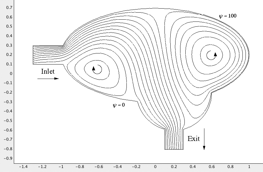
Fig. E7.4.5 Case 3. The river enters at AB and leaves at CD. A nonuniform wind blows, but because of the river flow the vortices are pushed into smaller areas.
7.6. Axially Symmetric Irrotational Flow3
3 The main goal of Sections 7.6–7.8 is to investigate flow around a sphere, needed in Chapter 10 when considering the rise of large bubbles in liquids and fluidized beds.
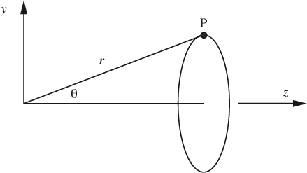
Another important class of potential flows occurs when there is rotational symmetry about an axis, an example being the flow of an otherwise uniform stream past a sphere or a spherical bubble. For these flows, it is basically convenient to employ spherical coordinates r and θ; the symmetry condition then reduces any derivatives in the azimuthal (φ) direction to zero. The coordinates are shown in Fig. 7.10(b), in which the axial direction z is that from which the angle θ is measured. Thus, we shall find ourselves working with r, θ, and z, but it is important to realize that these are not the usual cylindrical coordinates.
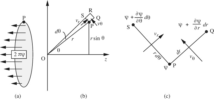
For this axisymmetric case, a new stream function ψ is now defined by reference to Fig. 7.10(a). Namely, the stream function at a point such as P is ψ if the flow rate is 2πψ, from right to left, through a circle formed by rotating P about the axis of symmetry. The factor of 2π is included because it will soon cancel with a similar quantity.
The two velocity components υr and υθ shown in Fig. 7.10(b) are now deduced by reference to Fig. 7.10(c). For example, the flow rate from right to left across the surface formed by rotating PS about the z axis is equal to 2π times the difference in stream functions at points S and P:
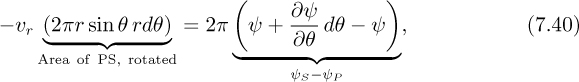
Similarly,
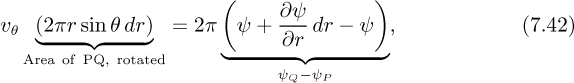
giving:
Since v = ∇φ, the velocities are given in terms of the potential φ by:
Continuity equation. Under steady-state conditions, there is no accumulation in the element PQRS in Fig. 7.10(b), so that:
or
which is the continuity equation in axisymmetric coordinates, identical to Eqn. (5.50), multiplied through by r2 sin θ. The reader may wish to check that the velocity components given in terms of the stream function in Eqns. (7.41) and (7.43) automatically satisfy Eqn. (7.46).
Irrotationality condition. The flow will be irrotational if the φ component of the vorticity is zero. From the entry in Table 5.4 under spherical coordinates, the irrotationality condition is obtained by setting the φ component of ∇ × v, which is normal to the plane containing υr and υθ, to zero:
Paralleling the x/y coordinate case, it may again be shown that the potential function in Eqn. (7.44) is compatible with this new irrotationality condition.
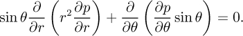
Laplace’s equation. Again paralleling the earlier x/y development, the velocity components derived from the velocity potential, which satisfies irrotationality, may be substituted into the continuity equation, (7.46), to give:

which is actually Laplace’s equation in spherical coordinates (see Table 5.5), multiplied through by r2 sin θ (and with zero derivative in the φ direction).
Likewise, if the stream function, which satisfies continuity, is substituted into the irrotationality condition, we obtain:

Although Eqn. (7.49) is a second-order differential equation in the stream function, it is no longer Laplace’s equation, nor a multiple of it.
7.7. Uniform Streams and Point Sources
We now examine a few cases of axisymmetric flows, for which it is convenient to use both the spherical and Cartesian coordinate frames, as shown in Fig. 7.11.
Uniform stream. A uniform stream flowing in the positive z direction with velocity U is shown in Fig. 7.12. By definition, the flow rate in the negative z direction through the circle of radius r sin θ passing through point P equals 2π times the stream function ψ at P:
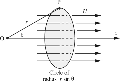
so that:
The velocity potential is found by integrating the relationships given in Eqn. (7.44):
which yield:
These last two expressions are compatible if f(θ) = g(r) = c, where c is a constant that is conveniently (but not necessarily) taken as zero, so that
As a scalar, φ is invariant to the coordinate system used. However, when using partial derivatives in two different coordinate systems, we must pay attention to which coordinates are being kept constant during partial differentiation. Observe also that ∂φ/∂z (with y constant) gives the z velocity component.
Point source. Fig. 7.13 shows a “point” source that emits a uniform flow in all radial directions. Its strength is defined as m if the total volumetric flow rate is 4πm, which also equals at any radius r the radial velocity υr times the surface area 4πr2 of the imaginary spherical shell through which the flow is passing:
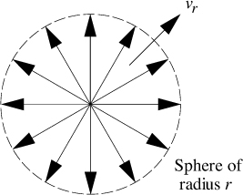
The radial velocity is therefore:
Observe that a point source by itself is not completely realistic, since the radial velocity is infinite at r = 0. Nevertheless, it is an important concept, as will be realized shortly. Integration of Eqn. (7.56) gives the velocity potential and stream function as:
(Arbitrary functions of integration can be shown to be constants—which may be taken as zero—by integrating the corresponding relationships for υθ, which is zero.)
Point source in a uniform stream. We now arrive at the intriguing possibility of combining the two previous concepts. As illustrated in Fig. 7.14, imagine a point source of strength m to be located at the origin O; superimposed on this flow is a uniform stream with velocity U flowing in the z direction. The previously derived velocity potentials and stream functions may be added, giving:
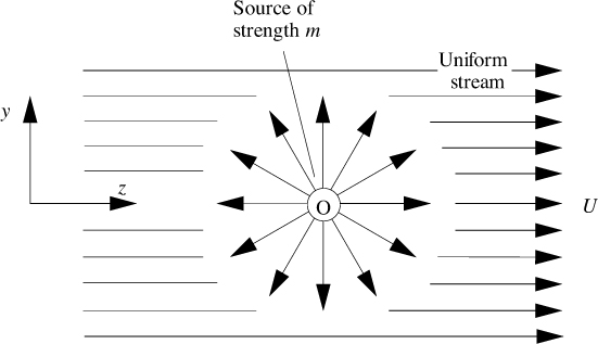
Fig. 7.14 Combination of a point source of strength m with a uniform stream of velocity U. The flow is axisymmetric about the z axis.
Observe from the diagram that the part of the source flowing to the left opposes and hence tends to “neutralize” the oncoming stream from the left. In fact, a stagnation point S, with zero velocity components (υr = υθ = 0), occurs when:
Therefore, as shown in Fig. 7.15, the stagnation point has coordinates:
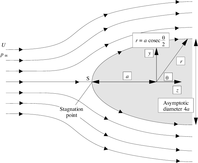
Fig. 7.15 The combination shown in Fig. 7.14 leads to axisymmetric irrotational flow around a blunt-nosed object.
in which the ratio of the source strength to the stream velocity has been replaced by the square of a new quantity, a.
From Eqns. (7.58) and (7.61), the value of the stream function at the stagnation point is ψ = –m = –Ua2. Therefore, the streamline passing through the stagnation point has the equation4:
4 This does not imply that the fluid actually flows through the stagnation point. As an infinitesimally small element of fluid approaches the stagnation point S along the streamline from the left, it continuously decelerates, and it may be shown that it takes an infinite time to reach S.
By using the identities:
the y and r coordinates of points on this streamline are found to be:
Equation (7.65) is drawn in Fig. 7.15 and is seen to be an axisymmetric curved surface with the stagnation point S at its “nose.” It therefore follows that the combination of a source in a uniform stream represents potential flow past an axisymmetric blunt-nosed body, whose asymptotic diameter can readily be shown to equal 4a. Of course, the equations also predict a flow pattern “inside” the body (what is it?), but we choose to ignore it here.
The pressure at any point can be obtained by first observing that the square of the velocity is:
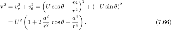
If the pressure in the undisturbed uniform stream (well away from the body) is p∞, then—apart from any hydrostatic effects—Bernoulli’s equation gives the local pressure at any point:

Clearly, by taking other combinations, more sophisticated flow patterns can be generated, but our purpose is just to make the reader aware of such possibilities. However, another interesting combination will be considered in the next section.
7.8. Doublets and Flow Past a Sphere
A doublet is very much like a dipole in electricity and magnetism, and is introduced in Fig. 7.16(a).
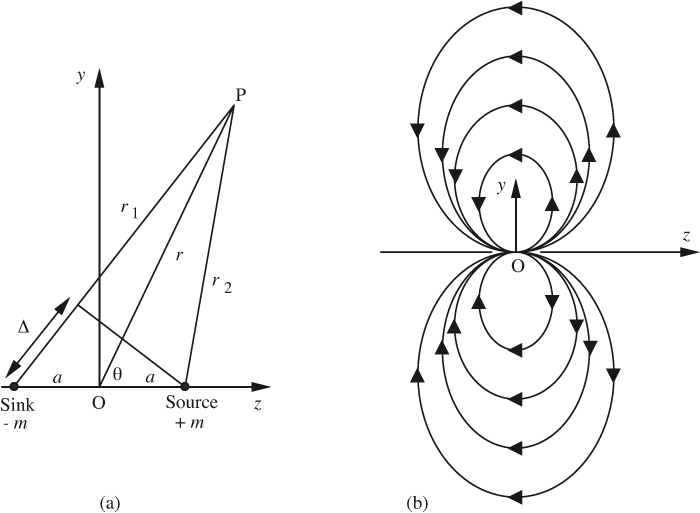
Fig. 7.16 (a) Point source and sink, which, when combined closely together lead to the flow from a doublet; (b) the resulting streamlines. The flow is axisymmetric about the z axis.
Consider a point source and a point sink of strengths m and –m, respectively, located on the z axis at distances a to the right and left of the origin. Fluid emanating from the source will eventually flow back into the sink. For the combination, the velocity potential at a point P is:
Now let a → 0 and m → ∞, but in such a way that the product 2am ≡ s remains finite, where s is known as the doublet strength, which will be positive when the direction from source to sink points in the negative z direction. The velocity potential becomes:
Following a similar argument, the stream function for the doublet is:
The corresponding streamlines are shown in Fig. 7.16(b).
Combination of a doublet and a uniform stream. In the same way the combination of a source and a uniform stream was investigated in the previous section, now consider the superposition of a doublet and a uniform stream.
Recall that for a uniform stream of velocity U in the z direction, the velocity potential and stream function are:
Also consider a doublet of strength s = –Ua3/2 at the origin, where U is again the velocity of the uniform stream and a is a variable whose significance is to be realized; the negative sign means that the orientation of the doublet is with the source to the left of the sink—opposite to that in Fig. 7.16:
Thus, for the combination of the uniform stream and the doublet:
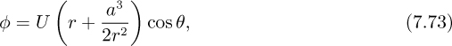
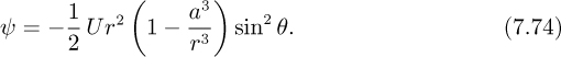
Investigation of Eqns. (7.73) and (7.74) leads to the following conclusions:
1. The streamline ψ = 0 occurs either for θ = 0 or π, or for r = a. Therefore, the sphere r = a may be taken as a solid boundary.
2. Both φ and ψ satisfy the general axisymmetric potential flow equations, (7.48) and (7.49).
3. Far away from the sphere, Eqns. (7.73) and (7.74) predict a uniform velocity U in the z direction.
4. These equations also predict a zero radial velocity υr at the surface of the sphere.
The combination of a uniform stream and a doublet (with directions opposed) represents potential flow of a uniform stream with a solid sphere placed in it, as shown in Fig. 7.17. This result will help us in Chapter 10 to predict the motion of bubbles in liquids and fluidized beds. Also see Example 12.3 for an application to electroosmotic flow around a particle in a microchannel.
7.9. Single-Phase Flow in a Porous Medium
Laplace’s equation also governs the flow of a viscous fluid, such as oil, in a porous medium, such as a permeable rock formation. Recall from d’Arcy’s law in Section 4.4 that the superficial velocity υx for one-dimensional flow is proportional to the pressure gradient:
where κ is the permeability of the medium and μ is the viscosity of the fluid. The minus sign occurs because the flow is in the direction of decreasing pressure. Equation (7.75) may be generalized to three-dimensional flow by using a vector velocity v and replacing dp/dx with the gradient of the pressure:
But for an incompressible fluid the continuity equation is:
The velocity may now be eliminated between these last two equations. If the permeability/viscosity ratio κ/μ is a variable, we obtain, after canceling the minus sign:
which simplifies in the case of constant κ/μ to:
That is, the pressure distribution is again governed by Laplace’s equation, which has been written out here for the case of two-dimensional rectangular coordinates, but is equally applicable in other coordinate systems. Thus, much of the theory in this chapter applies not only to flow of essentially inviscid fluids, but also to the flow of viscous fluids in porous media. Obvious important applications are to the recovery of oil from underground rock formations, and to the motion of groundwater in soil.
Example 7.5—Underground Flow of Water
A company has been disposing of some water containing a small amount of a chemical (1,4–dioxane) by injecting it into a permeable stratum of the ground via a vertical well, A, of radius a. Consequently, the groundwater has become slightly contaminated. As shown in Fig. E7.5.1(a), the company proposes to rectify the situation in a cleanup operation by drilling a second well, B, of the same radius, and separated by a distance L from A. Contaminated water will be withdrawn at a volumetric flow rate Q per unit depth from A, detoxified by irradiating it with ultraviolet light, and injecting the purified water back into the ground via well B. By modeling A as a line sink and B as a line source, derive an expression for the pressure difference pB – pA between the two wells, in terms of Q, a, L, κ, and μ. Sketch several streamlines and isobars.
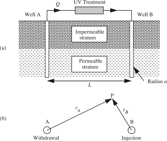
Fig. E7.5.1 Withdrawal and injection wells A and B: (a) shows the side view of a vertical section through the formation; (b) shows the plan of a horizontal section of the permeable stratum, together with the radial coordinates of point P.
Solution
For incompressible liquid flow in a porous medium, the superficial velocity vector (volumetric flow rate per unit area) v is given by d’Arcy’s law:
Laplace’s equation governs variations of pressure, which may be treated in virtually the same manner as the velocity potential in irrotational flow.
A plan of the permeable stratum is shown in Fig. E7.5.1(b), in which a general point such as P is seen to lie at radial distances rA and rB from the centers of wells A and B, respectively.
If B is considered to be a line source, with a total flow rate of Q per unit vertical depth (normal to the plane of Fig. E7.5.1(b)), the radially outward velocity υrB at any distance rB from it is obtained from continuity and d’Arcy’s law:
The corresponding pressure is obtained by integration:
For flow into the line sink at well A, the corresponding pressure is:
In these last two equations, the function of integration f(z) recognizes that the pressure also varies with the vertical distance z. Considering a fixed depth, the function effectively becomes a constant of integration, p0.
The combined effect of both injection and withdrawal wells leads to the pressure distribution:
in which the added pressure p0 depends on the depth of the stratum and the overall level to which it is pressurized.
Equation (E7.5.5) is next applied at the outer radius of each well in turn, namely, for rB = a, rA ![]() L (at well B) and rA = a, rB
L (at well B) and rA = a, rB ![]() L (at well A):
L (at well A):
The required pressure difference between the wells is therefore:
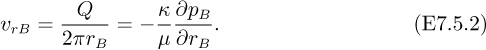
Finally, Fig. E7.5.2 shows several isobars (which are almost circular in the vicinity of the wells), together with the corresponding streamlines.
Fig. E7.5.2 Plan of a horizontal section through the permeable stratum, showing the streamlines (heavy) and isobars (light).
7.10. Two-Phase Flow in Porous Media
An important application of fluid mechanics is the study of the flow of crude oil in the pores of the porous rock formation in which it is found. Increasing amounts of oil can be recovered in several stages, including the following:
1. Primary recovery, in which as much oil is pumped out as possible.
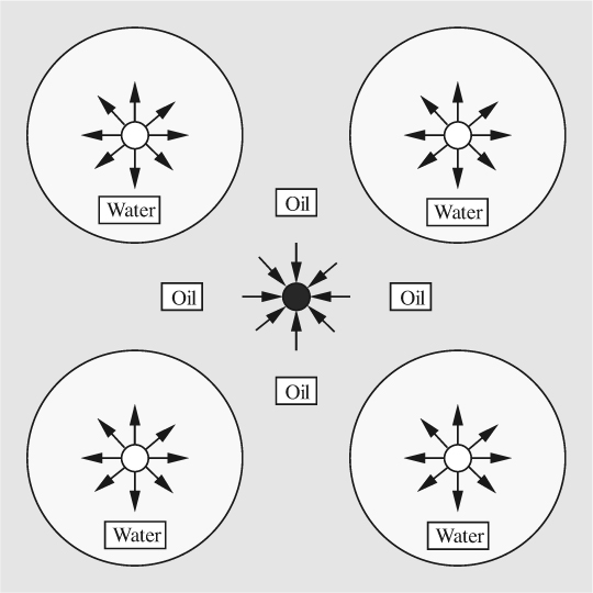
2. Secondary recovery, typically by pumping water down selected wells and displacing more of the oil, which is then produced at other selected wells. The “five-spot” pattern shown in Fig. 7.18 is frequently used. The duration of a single waterflood is many years, and it is usually important to simulate the results as accurately as possible beforehand, in order to maximize the production of oil. For example, if water is pumped down the wells too rapidly, it can “finger” towards the intended production wells, causing water to be “produced” instead of oil.
3. Tertiary recovery, in which surfactants are often used in order to reduce the capillary pressure between the oil and water, and to make it easier for the residual oil to be recovered.
The present discussion centers largely on secondary recovery, in which water and oil flow as two immiscible phases. Similar equations also govern the underground storage of natural gas, typically by the displacement of naturally occurring water. The notation to be used is given in Table 7.2.
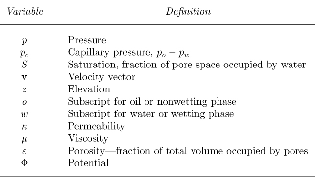
d’Arcy’s law can be applied to each of the two phases:
in which the fluid potentials combine both the pressure and hydrostatic effects:
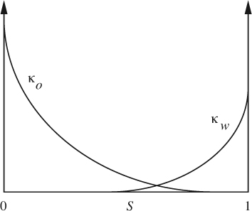
In Eqns. (7.80) and (7.81), the permeabilities are strong functions of the water saturation, relative values being shown in Fig. 7.19; typical maximum values are in the range of 10–100 md (millidarcies). Observe that each permeability is zero over a significant range of saturations; water will not flow unless its saturation reaches a certain threshold, and neither will the oil.
The capillary pressure is the excess pressure in the nonwetting phase over that in the wetting phase:
and is again a strong function of the water saturation, as shown in Fig. 7.20(c). There, the normalized saturation ![]() is shown, with the following extreme values:
is shown, with the following extreme values:
1. For connate water (the water initially present in the oil-containing formation), ![]() = 0.
= 0.
2. For residual oil (the residual oil when a porous medium containing oil is displaced by water), ![]() = 1.
= 1.
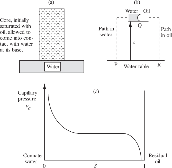
Capillary pressure may be determined as shown in Fig. 7.20(a), by allowing a rock core, previously saturated with oil, to contact water at its base. Capillary attraction will cause the water to rise into the core, where its saturation will vary with elevation z.
If the path PQR is traversed, as shown in Fig. 7.20(b), the overall pressure change must be zero, since pR = pP:
If the water contains a small amount of an electrolyte such as sodium chloride, electrical conductivity measurements enable the saturation to be determined at various values of z, and hence pc as a function of S or ![]() .
.
Volumetric balances (the density is constant) on unit volumes give:
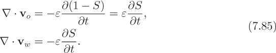
Substitution of the velocities from Eqns. (7.80) and (7.81) gives:
Note that the time derivative of the saturation may be reexpressed in terms of the derivative of the potential difference:
in which S′ = dS/dpc may be obtained by measuring the slope of the capillary-pressure curve at the appropriate value of the saturation.
With the above in mind, the transport equations become:


Eqns. (7.89) and (7.90) must be solved numerically, and an appropriate rearrangement is to define sums and differences of the potentials and mobilities as:
so that Eqns. (7.89) and (7.90) can be rewritten as:
These last two equations are of elliptic and parabolic type, respectively, and may be solved by standard numerical techniques such as successive overrelaxation and the implicit alternating-direction method, as performed, for example, by Goddin et al.5
5 C.S. Goddin, Jr., F.F. Craig, M.R. Tek, and J.O. Wilkes, “A numerical study of waterflood performance in a stratified system with crossflow,” Journal of Petroleum Technology, Vol. 18, pp. 765–771 (1966). Also see Chapter 7 of B. Carnahan, H.A. Luther, and J.O. Wilkes, Applied Numerical Methods, Wiley & Sons, New York, 1969.
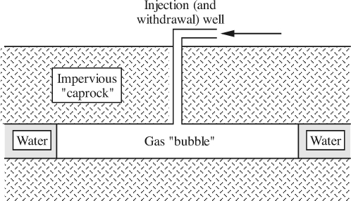
Underground storage of natural gas. Several areas in the northern United States rely largely on the southern and southwestern part of the country for their supply of natural gas, which is typically conveyed by pipelines over distances sometimes amounting to 1,000–2,000 miles. Year-round operation of these pipelines is desirable in order to minimize costs. However, the consumer demand for the gas fluctuates substantially from a low point during the summer to a maximum during the winter. The excess gas pumped during the summer is most conveniently stored in underground porous-rock formations—preferably in depleted gas or oil fields, since these are known to be surmounted by an impermeable “caprock” formation that will prevent leakage.
The general scheme is shown in Fig. 7.21; the storage region is usually dome-shaped, with its highest elevation near the well or wells, thereby trapping the gas and preventing it from escaping laterally. During the summer, gas is pumped down one or more wells into the porous formation, whose storage region is called the gas “bubble,” even though its horizontal extent may be thousands of feet. For the storage region, a typical vertical thickness is 100 ft, with a permeability in the range of 50–500 md. As the gas is injected, it displaces naturally occurring water laterally. During the winter, the gas is withdrawn, and the water moves back.
The annual cycles of gas and water movement are governed by equations very similar to those already outlined for oil and water. However, significant additional simplifications may also be made because the gas and water regions can usually be treated realistically as single-phase regions. The following is a typical equation that governs pressure variations p(x, y, t) of the gas, in which x and y are coordinates in the horizontal plane of the gas bubble and t is time:

Here, M(x, y) is the local mass withdrawal rate of gas per unit volume (which will be zero if there is not a well in the vicinity), h(x, y) is the local formation thickness, κ(x, y) is the local permeability, z is the compressibility factor of the gas, μ is the viscosity, T is the absolute temperature, Mw is the molecular weight of the gas, ε is the porosity or void fraction, and R is the gas constant.
7.11. Wave Motion in Deep Water
This chapter concludes with another, and quite different, application of potential flow theory—the motion of waves on an open body of water. We wish to find how the velocity of the water varies with time and position below the free surface.
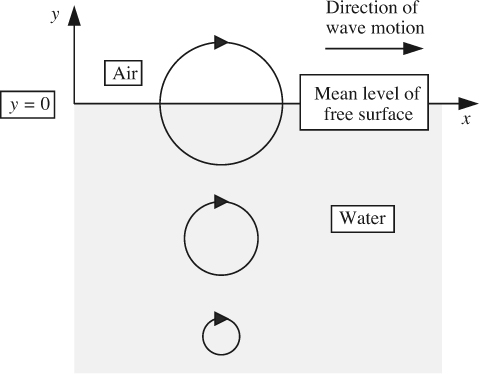
Fig. 7.22 shows a continuous wave that is moving to the right (in the x direction) on the surface of a body of very deep water of negligible viscosity. The equation of the free surface is:
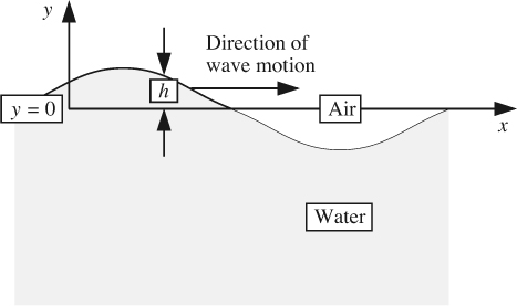
in which a is the amplitude, λ is the wavelength, k = 2π/λ is the wave number, ω is the circular frequency, c = ω/k is the velocity of wave propagation, and the origin y = 0 corresponds to the level of the surface in the absence of waves.
The following potential function has been proposed for the motion of the water:
which satisfies Laplace’s equation, since:

Note that in the very deep part of the water, y becomes highly negative, and the potential function and velocities approach zero.
Equation (7.8), for inviscid, irrotational, yet transient flow, with y now representing the vertical coordinate, leads to:
That is, any variation of the quantity in parentheses will generate a corresponding rate of change in the velocity. The substitution v = ∇φ, coupled with the fact that the order of the gradient and partial differential operations can be interchanged, yields:
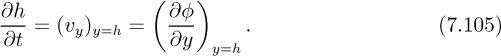
Eqn. (7.100) is now applied at the free surface, y = h. For waves of small amplitude, the kinetic energy term can be neglected, giving:
Noting that the pressure is a constant at the free surface, differentiation of Eqn. (7.101) with respect to time gives:
The free surface is described by the equation h = y. Since a point on the surface moves with the liquid, we can employ differentiation following the liquid—that is, involve the substantial derivative, giving:
or,
The terms on the left-hand side of Eqn. (7.104) have the following physical interpretations:
1. The first term, ∂h/∂t, represents the rate at which the elevation of the free surface itself is increasing.
2. The second term, υx(∂h/∂x), represents the rate of increase of elevation of a fluid particle that is traveling with velocity υx and is constrained to follow the contour of the free surface.
The combined effect then gives the actual y component of velocity, υy. The situation is very much like the rate of increase of elevation of a person running up a hill, if the hill itself is moving upward, perhaps due to an earthquake.
For waves of small amplitude, the term involving the slope ∂h/∂x is small and can be neglected, resulting in:
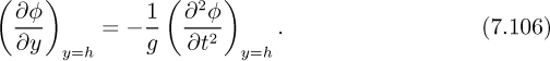
Elimination of ∂h/∂t between Eqns. (7.102) and (7.105) gives:
For the known potential function of Eqn. (7.97), these last two derivatives may be evaluated, leading to:
But since the velocity of the waves is c = ω/k and k = 2π/λ, it follows that:
giving not only the wave velocity but also demonstrating that waves of long wavelength travel faster than those of short wavelength. For a combination of waves of different wavelengths, there is a dispersion between the various wavelengths.
Finally, investigate the paths followed by individual liquid particles. By differentiation of the potential function, the velocity components—referred to the location x = 0 for simplicity—are:
As ωt varies, the distances traveled in the x and y directions by a liquid particle can be obtained by integration of Eqns. (7.109) and (7.110) with respect to time:
We can choose a starting point such that the constants of integration are both zero, and deduce from Eqn. (7.111) that:

That is, any liquid particle travels in a circle of radius aeky, which diminishes rapidly with depth away from the free surface, as shown in Fig. 7.23. In particular, note that the radius of motion at the free surface (y = 0) equals—as it must—the amplitude a of the passing wave.
Problems for Chapter 7
Unless otherwise stated, all flows are steady state, with constant density and viscosity (the latter for porous-medium flows).
1. Flow past a sphere—M. Consider the velocity potential and stream function for inviscid flow of an otherwise uniform stream U past a sphere of radius a, as given by Eqns. (7.73) and (7.74). Verify that these functions:
(a) Satisfy the appropriate axially symmetric equations, (7.48) and (7.49).
(b) Predict a uniform velocity U in the z direction far away from the sphere.
(c) Predict a zero radial velocity υr at the surface of the sphere.
(d) Give a streamline ψ = 0 either for θ = 0 or π, or for r = a, showing that the sphere r = a may be taken as a solid boundary.
2. Continuity and irrotationality—E. Verify the following for irrotational flow in x/y coordinates:
(a) That the velocity components, defined in Eqn. (7.14) in terms of the velocity potential, automatically satisfy the irrotationality condition and—when substituted into the continuity equation—lead to Laplace’s equation in φ.
(b) That the velocity components, defined in Eqn. (7.17) in terms of the stream function, automatically satisfy the continuity equation and—when substituted into the irrotationality condition—lead to Laplace’s equation in ψ.
3. Flow past a cylinder—E. Consider the velocity potential and stream function for inviscid flow of an otherwise uniform stream U past a cylinder of radius a, as given by Eqns. (7.30) and (7.31). Verify that these functions:
(a) Satisfy Laplace’s equations, (7.32).
(b) Predict a uniform velocity U in the x direction and zero velocity in the y direction far away from the cylinder.
(c) Give a streamline ψ = 0 either for θ = 0 or π, or for r = a, showing that the cylinder r = a may be taken as a solid boundary. Also prove that υr = 0 at r = a.
4. Stagnation and other flow—E. Answer the following two parts:
(a) Derive the velocity potential function φ(x, y) for the stagnation flow whose stream function is given in Eqn. (E7.2.1) as ψ = cxy. Sketch several streamlines and equipotentials.
(b) For a certain flow, the velocity potential is given by:
φ = ax + by.
Give physical interpretations of a and b, derive the corresponding stream function, ψ(x, y), and sketch half a dozen streamlines and equipotentials.
5. Axisymmetric continuity and irrotationality—E. For axially symmetric ir-rotational flows, verify the following:
(a) That the velocity components, defined in Eqn. (7.44) in terms of the velocity potential, automatically satisfy the irrotationality condition and—when substituted into the continuity equation—lead to Eqn. (7.48) in φ.
(b) That the velocity components, defined in Eqns. (7.41) and (7.43) in terms of the stream function, automatically satisfy the continuity equation and—when substituted into the irrotationality condition—lead to Eqn. (7.49) in ψ.
6. Uniform flow, point source, and line sink—M. Fig. P7.6 shows a line source, in which the total strength m is distributed evenly along the z axis between the origin O and the point z = a. Thus, an element of differential length dζ of this source will have a strength mdζ/a, and the corresponding stream function at a point P, whose coordinates are (r, θ), will be:
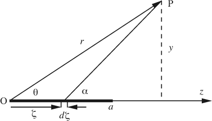
Prove by integration between ζ = 0 and ζ = a for this axisymmetric flow problem that the stream function at P due to the entire line source is:
Now consider the effect of a combination of the following three items:
(a) A uniform flow U in the z direction.
(b) A point source of strength m at the origin.
(c) A line sink of total strength m, extending between the origin O and a point z = a on the axis of symmetry.
Derive an expression for the stream function ψ at any point, indicate what type of flow this represents, and sketch a representative sample of streamlines.
7. Tornado flow—M. This problem is one in axisymmetric cylindrical coordinates. Derive the velocity potential function for the following two flows:
(a) A free vortex, centered on the origin, in which the only nonzero velocity component is υθ = α/r.
(b) A line sink along the z axis, in which the only nonzero velocity component is υr = –β/r.
Hint: Remember to involve the components of ∇φ in cylindrical coordinates.
Sketch a few streamlines for a tornado, which can be approximated by the following combination:
(a) A free vortex, centered on the origin at r = 0.
(b) A line sink flow, towards the origin.
At a distance of r = 2, 000 m from the “eye” (center) of a tornado, the pressure is 1.0 bar and the two nonzero velocity components are υr = –0.25 m/s and υθ = 0.5 m/s. The density of air is 1.2 kg/m3. At a distance of r = 10 m from the eye, compute both velocity components and the pressure. What is likely to happen to a house near the center of the tornado?
8. Spherical hole in a porous medium—M. The velocity v of a liquid percolating through a porous medium of uniform permeability κ under a pressure gradient is given by d’Arcy’s law:
For an axially symmetric flow, you may assume that the corresponding superficial velocity components are:
in which r and θ are spherical coordinates. Prove that the pressure p obeys the following equation:
Water seeps from left to right through a porous medium that is bounded by two infinitely large planes AB and CD, separated by a distance 2L, and whose pressures are P and – P, respectively, as shown in Fig. P7.8.
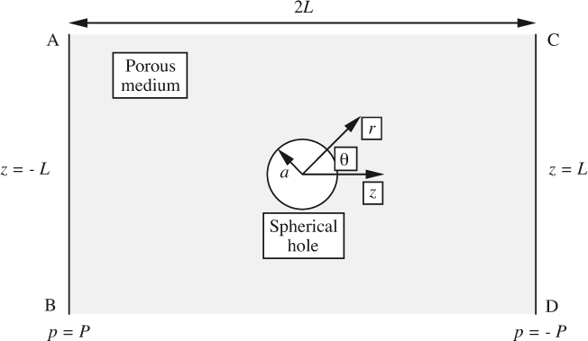
Halfway across, the medium contains a spherical hole of radius a, which offers no resistance to flow, and in which the pressure is p = 0. The dimensions are such that a/L ≪ 1.
Show that the pressure distribution is given approximately by:
and then determine the coefficients α and β in terms of L, P, and a. Hint: Check that this expression for p satisfies the governing differential equation and all boundary conditions.
Also, sketch a few streamlines and prove that the volumetric flow rate of water through the hole is:
If needed, sin 2θ = 2 sin θ cos θ. (A very closely related problem occurs during the upwards motion of bubbles in a fluidized bed of catalyst particles, in which a significant amount of the fluidizing gas sometimes “channels” through the bubbles and hence has an adversely reduced contact with the catalyst.)
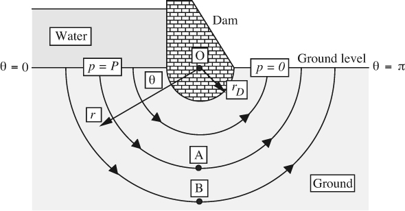
9. Seepage under a dam—M. The (vector) superficial velocity of an incompressible liquid of constant viscosity μ percolating through a porous medium of uniform permeability κ is given by d’Arcy’s law:
where p is the pressure beyond that occurring due to usual hydrostatic effects.
(a) In one or two sentences, state why you would expect the flow to be irrotational.
(b) Use the vector form of the continuity equation to show that the excess pressure obeys Laplace’s equation, ∇2p = 0. (Note that in this case the excess pressure behaves very much like the velocity potential φ in irrotational flow, in which the Laplacian of φ is also zero.)
Fig. P7.9 shows seepage of water through the ground under a dam, caused by the excess pressure P that arises from the buildup of water behind the dam, which has (underground) a semicircular base of radius rD. The following relation has been proposed for the excess pressure in the ground:
(c) Prove that Eqn. (P7.9.2) is correct by verifying that it satisfies:
(i) The conditions on pressure at the ground level.
(ii) Laplace’s equation, ∇2p = 0, in cylindrical (r/θ/z) coordinates, in which all z derivatives are zero.
(iii) Zero radial flow at the base of the dam.
(d) What are the r and θ components of ∇p in cylindrical (r/θ/z) coordinates? What then are the expressions for υr and υθ in terms of r and θ? If the corresponding expressions in terms of the stream function ψ are:
derive an expression for the stream function in terms of r and/or θ, and hence prove that the streamlines are indeed semicircles. Draw a sketch showing a few streamlines and isobars (lines of constant pressure—much like equipotentials).
(e) Between points A and B, some copper-impregnated soil has been detected, with the possibility that some of this toxic metal may leach out and have adverse effects downstream of the dam. To help assess the extent of this danger, derive an expression for the volumetric flow rate Q of water between A and B (per unit depth in the z direction, normal to the plane of the diagram). Your answer should give Q in terms of P, κ, μ, rA, and rB.
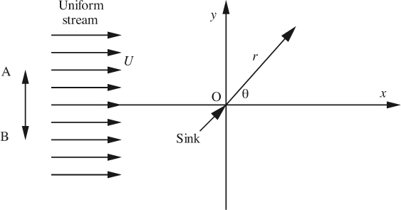
10. Uniform stream and line sink—M. In this two-dimensional problem, give your answers in terms of r and θ coordinates, except in one place where the y coordinate is specifically requested.
(a) A line sink at the origin O extends normal to the plane shown in Fig. P7.10. If the total volumetric flow rate withdrawn from it is 2πQ per unit length, prove that the velocity potential is:
φ = –Q ln r.
What is the corresponding equation for the stream function ψ?
(b) Now consider the addition of a stream of liquid, which far away from the sink has a uniform velocity U in the x direction. Show for the combination of uniform stream and sink that φ = Ur cos θ – Q ln r, and also obtain the corresponding expression for ψ.
(c) Give expressions for the velocity components υr and υθ, and from them demonstrate that the flow is irrotational.
(d) Where is the single stagnation point S located? What is the equation of the streamline that passes through S? Hence, by considering the y coordinate of this streamline far upstream of the sink, deduce, in terms of U and Q, the width AB of that portion of the uniform stream that flows into the sink.
(e) Sketch several equipotentials and streamlines for the combination of uniform stream and sink.
(f) For incompressible liquid flow in a porous medium, the superficial velocity vector (volumetric flow rate per unit area) v is given by d’Arcy’s law:
in which κ is the uniform permeability, μ is the constant viscosity, and p is the pressure. Prove that the pressure obeys Laplace’s equation:
∇2p = 0,
so that it may be treated essentially as the velocity potential that we have been studying for irrotational flow, the only difference being the factor of –κ/μ. Hence, if Fig. P7.10 now represents the horizontal cross section of a well in a porous soil formation, derive an expression showing how the pressure p deviates from its value pS at the stagnation point.
11. Injection well near an impermeable barrier—M. This problem involves potential flow in two dimensions—not in axisymmetric spherical coordinates. For convenience, both the x, y and r, θ coordinate systems will be needed.
(a) First consider a line source at the origin O, extending normal to the x, y plane. The flow is radially outwards everywhere (with υθ = 0), and the total volumetric flow rate issuing from the source is 2πQ per unit depth (corresponding to a strength Q). Deduce a simple expression for the radial velocity υr as a function of radial distance r, and hence prove that the velocity potential is given by:
φ = Q ln r.
What is the corresponding equation for the stream function ψ?
(b) Derive an expression for the time t taken for a fluid particle to travel from the source to a radial location where r = R.
(c) Next, Fig. P7.11(a) shows a line source located at point B, which has coordinates x = a and y = 0. There is an impermeable barrier to flow along the plane Y–Y, which extends indefinitely along the y axis. Explain why the potential φ and stream function ψ at a point P, with coordinates (x, y), may be modeled by adding to the source B an identical source of strength Q, but now located at a point A with coordinates x = –a and y = 0.
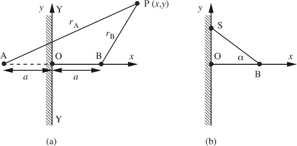
(d) For the combination of the two sources, obtain an expression for the stream function at point P in terms of Q, x, and y. Assume the following identity if needed:

(e) Sketch several streamlines (for x ≥ 0 only), clearly showing the direction of flow. If there is a stagnation point, identify it. If there isn’t one, explain why not.
(f) Write down an expression for the potential function φ at point P in terms of Q, rA, and rB. Add several equipotentials to your diagram.
(g) Fig. P7.11(b) shows the same basic situation, but with several lines removed for clarity. Consider the velocity υy (in the y direction) at a point S on the barrier. For what value of α would υy be a maximum? Explain.
(h) Suppose now that there is a well W of radius R centered on B (where R ≪ a), situated in a porous formation of permeability κ, and into which treated waste water of viscosity μ is being injected at a volumetric flow rate Q. Derive an expression for pW – pO, the pressure difference between well W and the origin O. Hint: recall that flow through a porous medium may be modeled as potential flow, provided that φ is replaced by –κp/μ.
12. Circulation in vortices—E. By examining the appropriate component of curl v, derive expressions for the circulation—defined in Eqn. (5.26)—in the forced-and free-vortex regions of Example 7.1, and comment on your findings.
13. Motion of a particle in potential flow—D. This problem has applications in the sampling of fluids for entrained particles. First, examine Example 7.3. A small spherical particle of diameter dp and density ρp enters upstream of the slot at a location to be specified, with initial (t = 0) velocity components (![]() ,
, ![]() ). The particle is sufficiently small so that Stokes’ law gives the drag force on it:
). The particle is sufficiently small so that Stokes’ law gives the drag force on it:
in which μf is the viscosity of the fluid, and superscripts f and p denote fluid and particle velocities, respectively.
Prove that the following dimensionless differential equations give the accelerations of the particle in the two principal directions:
in which:

Use a spreadsheet, MATLAB, or other computer software to determine the subsequent location of the particle (measured by X and Y) as a function of time, starting from τ = 0 and proceeding downstream until either: (a) the particle enters the slot, (b) the particle hits the wall, or (c) the particle proceeds beyond the slot and has an insignificant value of ![]() . Euler’s method with a time step of Δτ is suggested for solving the differential equations (see Appendix A).
. Euler’s method with a time step of Δτ is suggested for solving the differential equations (see Appendix A).
If you use a spreadsheet, the following column headings are suggested for tracking the various quantities over successive time steps: τ, X, Y, ![]() ,
, ![]() ,
, ![]() ,
, ![]() ,
, ![]() , and
, and ![]() .
.
Take Y0 large enough so that its exact value is not critical. Plot four representative particle trajectories for various values of X0 and ξ, and give comments with a few sentences on each trajectory.
14. Packed-column flooding—D (C). Consider the upward flow of an essentially inviscid gas of density ρG around a sphere of radius a. Well away from the sphere, the upward gas velocity is U, so the stream function is:
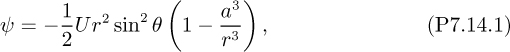
in which r is the radial distance from the center of the sphere and the angle θ is measured downward from the vertical. Derive a relation for ![]() as a function of r and θ. Hence, prove that the pressure gradient in the θ direction at the surface of the sphere is:
as a function of r and θ. Hence, prove that the pressure gradient in the θ direction at the surface of the sphere is:
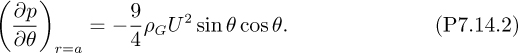
In an experiment to investigate the flooding of packed columns (the inability to accommodate ever-increasing simultaneous downward liquid flows and upward gas flows), an inviscid liquid of density ρL flows freely and symmetrically under gravity as a thin film covering the surface of a solid sphere. Gas of density ρG flows upward around the sphere, and its stream function is given by Eqn. (P7.14.1).
By considering the equilibrium of a liquid element that subtends an angle dθ at the center, show that the pressure gradient within the gas stream will prevent the liquid from running down when:
and that this will first be satisfied when:
15. Vortex lines and streamlines—E. Consider the forced vortex region of a stirred liquid, as in Example 7.1. Ignoring gravitational effects, what is the shape of the surface on which p/ρ + v2/2+ gz is constant? Illustrate with a sketch, showing the direction of the velocity and the vorticity at a representative point, together with the direction in which p/ρ + v2/2+ gz is increasing.
16. Velocity potential/stream function—M (C). In a certain two-dimensional irrotational flow, the velocity potential is given by:
φ = a(x2 + by2),
where a = 0.1 s–1.
Evaluate the constant b, and derive an expression for the corresponding stream function. Considering only the region x > 0, y > 0, sketch a few typical streamlines and hence determine the flow pattern that φ represents.
If at time t = 0 an element of fluid is at the point P (x = 10 cm, y = 20 cm), find its position Q at a time t = 2 s, and illustrate its path on your diagram.
17. Flow of water between two wells—M. For the situation shown in Example 7.4, take the following values: μ = 1 cP, κ = 15 darcies, a = 0.05 m, and L = 1,000 m. If the available pump limits the pressure drop between the two wells to 5.0 bar, what volumetric flow rate of water can be expected per unit vertical depth of the stratum? Give your answer in both cubic meters per second per meter depth, and in gpm per foot depth.
Under these conditions, what is the superficial velocity (m/s) of the water at a point exactly halfway between the two wells? With this velocity, how far would the water travel in a year if the stratum has a porosity of 0.30?
18. Effect of waves below the surface—E. Parallel waves whose peaks are spaced 5 m apart are traveling continuously on the surface of deep water. What is the velocity (m/s) of these waves? At what depth below the surface will the magnitude of the displacement be one-hundredth of its value at the surface?
19. Sampling a fluid—M. An axisymmetric inviscid incompressible flow consists of the combination of two basic elements:
(i) A uniform stream of fluid with velocity U in the positive z direction.
(ii) A point sink located at the origin, r = 0, that withdraws a sample of the fluid at a steady volumetric flow rate 4πQ.
For the combined two flows:
(a) Give expressions in spherical coordinates (r and θ) for the stream function and potential function.
(b) Sketch several streamlines and equipotentials. Show all relevant details.
(c) From the stream function, deduce the corresponding velocity components, υr and υθ.
(d) Is there a stagnation point? If so, explain where it is located and why. If not, explain why not.
(e) Below what radius a, measured in the y direction, will fluid coming from a large distance in the negative z direction be withdrawn by the sampling point? The y and z coordinates are those shown in Fig. 7.11 of your notes.
(f) Consider a small element of the fluid starting at an upstream point (z = –D; y = H). Explain carefully how would you determine the time taken for it to reach the sink. You need not carry the derivation completely to its conclusion, but you should give sufficient detail so that—given enough time—it could be completed by somebody else.
20. Storage of natural gas—E. Prove Eqn. (7.95), for the pressure variations in the gas bubble during the underground storage of natural gas. A transient balance on an element of dimensions dx × dy × h is recommended.
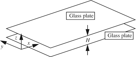
21. Hele-Shaw flow—M Flow of a liquid of viscosity μ occurs between two parallel horizontal transparent glass plates separated by a small distance H, as shown in Fig. P7.21. The plates are sealed around the edges to prevent leakage, except for small ports where the liquid may be introduced and withdrawn. By adding dye or small tracer particles, flow patterns may be observed by looking down through the top plate—including flows past obstacles that may be clamped between the plates. The object of this problem is to show that even though the flow is viscous, the mean velocity components ![]() and
and ![]() in the horizontal x/y plane are the gradients of a scalar φ—that is, the flow behaves as though it were irrotational, and the corresponding streamlines can be observed.
in the horizontal x/y plane are the gradients of a scalar φ—that is, the flow behaves as though it were irrotational, and the corresponding streamlines can be observed.
The x velocity component obeys the simplified momentum equation:
where z is the vertical coordinate measured normal to the plates (with z = 0 at the midplane). A similar equation holds for the y velocity component.
(a) State the simplifying assumptions that Eqn. (P7.21) implies.
(b) Derive an expression for υx in terms of H, z, μ, and ∂p/∂x, and for ![]() (the mean value of υx between the two plates) in terms of H, μ, and ∂p/∂x.
(the mean value of υx between the two plates) in terms of H, μ, and ∂p/∂x.
(c) Write down, without proof, the corresponding expression for the mean y velocity component ![]() .
.
(d) What is the potential function φ that gives ![]() = ∇φ, the velocity vector whose components are
= ∇φ, the velocity vector whose components are ![]() and
and ![]() ?
?
22. Flow pattern for wells—M. The Hele-Shaw apparatus of Problem 7.21 is to be used for simulating the porous-medium flow in a horizontal plane (viewed from above in Fig. P7.22) between one injection well I and two withdrawal wells A and B (which share equally the flow rate injected, but which do not necessarily have the same pressure). The situation is very similar to that of Example 7.5, except that there are now two withdrawal wells and there is an impermeable boundary surrounding the region.
(a) Explain briefly why the Hele-Shaw apparatus can simulate flow in a porous medium.
(b) Sketch the flow patterns that are likely to result, as follows:
(i) Eight streamlines (full curves with arrows) and six isobars or equipotentials (dotted curves) are expected, on a full-page diagram.
(ii) Do not perform any calculations or algebra.
(iii) Make sure you give reasonable coverage to the whole area—not just in the vicinity of the wells.
(iv) Identical streamlines obtained from symmetry should be included, but will not contribute to the total of eight required.
(v) Clearly indicate with the letter “S” (stagnation) any points where the velocity is zero.
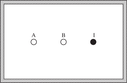
23. Flow in wedge-shaped region—M. Verify that the potential function:
φ = –cr3 cos 3θ,
with c a constant, gives two-dimensional irrotational flow in the wedge-shaped region that is bounded by the planes θ = 0 and θ = π/3. Sketch a few streamlines, clearly showing the direction of flow. Is there a stagnation point? If so, where?
24. Inviscid flow with rotation—E. Referring to Example 7.5:
(a) Prove the validity of –∇2ψ = ζ, where ζ = (∂υy/∂x – ∂υx/∂y) is the vorticity.
(b) Does the use of –∇2ψ = ζ still imply that continuity is satisfied?
25. True/false. Check true or false, as appropriate:
(a) Euler’s equation arises when inertial effects are ignored, but viscous effects are included.
T ![]() F
F ![]()
(b) In a forced vortex, the velocity component υθ is uniform everywhere.
T ![]() F
F ![]()
(c) It is possible to have an irrotational flow in which the fluid is everywhere moving in concentric circles.
T ![]() F
F ![]()
(d) Angular velocity is twice the vorticity.
T ![]() F
F ![]()
(e) Velocities given in terms of the potential function by υx = ∂φ/∂x and υy = ∂φ/∂y automatically satisfy the continuity equation.
T ![]() F
F ![]()
(f) Streamlines can cross one another.
T ![]() F
F ![]()
(g) Velocity components may be deduced from expressions for either the velocity potential or the stream function.
T ![]() F
F ![]()
(h) The stream function ψ = Ux represents a uniform flow in the x direction.
T ![]() F
F ![]()
(i) The problem of irrotational flow past a cylinder is best solved in axisymmetric spherical coordinates.
T ![]() F
F ![]()
(j) In a potential flow solution, the velocity must always be zero on a solid boundary.
T ![]() F
F ![]()
(k) The stream function for axisymmetric irrotational flows satisfies Laplace’s equation.
T ![]() F
F ![]()
(l) A point source of strength m emits a total volumetric flow of m per unit time.
T ![]() F
F ![]()
(m) Simple potential flows may be combined with one another in order to simulate more complex flows.
T ![]() F
F ![]()
(n) A stagnation point occurs when the pressure becomes a minimum.
T ![]() F
F ![]()
(o) A fluid doublet has equal effects in all directions.
T ![]() F
F ![]()
(p) The combination of a doublet and a uniform stream, with directions opposed to each other, represents ir-rotational flow past a solid sphere.
T ![]() F
F ![]()
(q) In the forced vortex of Fig. 7.1(a), the shear stress τrθ is zero.
T ![]() F
F ![]()
(r) For flow parallel to the x axis, as shown in Fig. 7.7, the stream function decreases in the y direction.
T ![]() F
F ![]()
(s) The radial velocity at a distance from a point source of strength m is given by υr = m/r.
T ![]() F
F ![]()
(t) Tornado flow can be approximated by a combination of a line sink and a forced vortex.
T ![]() F
F ![]()
(u) When waves of a given amplitude travel on the surface of water, those having higher values of ω will have a larger effect on the velocities at greater depths than waves with lower values of ω.
T ![]() F
F ![]()
(v) In the theoretical treatment of potential flow past a cylinder, the solution must satisfy zero tangential velocity υθ at the surface of the cylinder.
T ![]() F
F ![]()
(w) Laplace’s equation governs the pressure distribution for steady single-phase flow in a porous medium.
T ![]() F
F ![]()