
Chapter 14. COMSOL (FEMLAB) Multiphysics for Solving Fluid Mechanics Problems
14.1. Introduction to COMSOL Multiphysics
Chapter 13 introduced the general concept and importance of computational fluid dynamics (CFD), together with the three main types of programs (based on the FDM, FEM, and FVM). The chapter concluded with four illustrations of the versatile capabilities of FlowLab, which is based on the finite-volume method.
The present chapter introduces COMSOL Multiphysics (which we shall usually abbreviate as “COMSOL”), another type of CFD software, which is based on the finite-element method. COMSOL (known as FEMLAB until September 2005, when COMSOL 3.2 was introduced) is developed by COMSOL Inc., and its broad capabilities are best introduced by quoting (with permission) several paragraphs (until the middle of the next page) from the earlier FEMLAB 3 User’s Guide:
“FEMLAB is designed to make it as easy as possible to model and simulate physical phenomena. With FEMLAB, you can perform free-form entry of custom partial differential equations (PDEs) or use specialized physics application modes. These physics modes consist of predefined templates and user interfaces that are already set up with equations and variables for specific areas of physics. Further, by combining any number of these application modes into a single problem description, you can model a multiphysics problem—such as one involving simultaneous mass and momentum transfer.
The Model Library is an essential part of the package. It contains complete models taken from various engineering fields, including a special Chemical Engineering Library Module. Each model includes extensive documentation. Because the models already come with the finite-element mesh and the solution, you can immediately try out various postprocessing options.
Since its introduction in 1999, FEMLAB has been fully integrated with MATLAB. In fact, until the release of FEMLAB version 3.0, MATLAB was required, although this is no longer the case. Even so, those who wish to run FEMLAB along with MATLAB can do so through a new interface that make it possible to do FEMLAB script programming within the MATLAB language.
FEMLAB is a powerful, interactive environment for modeling and solving all kinds of scientific and engineering problems that are governed by partial differential equations (PDEs). By using the built-in physics modes it is possible to build models by defining the relevant physical quantities such as material properties, loads, constraints, sources, and fluxes, rather than by defining the underlying equations. FEMLAB then internally compiles a set of PDEs representing the entire model. You access FEMLAB as a stand-alone product through a flexible graphical user interface (GUI) or by script programming in the MATLAB language.
The underlying FEMLAB structure is a system of PDEs, three ways of describing these being:
• Coefficient form, suitable for linear or nearly linear models.
• General form, suitable for nonlinear models.
• Weak form, useful for models with PDEs on boundaries or those using terms with mixed space and time derivatives.
With these application modes, you can perform various types of analysis, including:
• Eigenfrequency and modal analysis.
• Stationary and time-dependent analysis.
• Linear and nonlinear analysis.
FEMLAB can solve a very wide range of problems, including those in fluid dynamics, chemical reactions, electromagnetics, fuel cells and electrochemistry, transport phenomena, polymer processing, and so on.”
COMSOL, as discussed in the present chapter, affords an ideal entry point to the realm of CFD, for the following reasons:
• Its interface is easy to use.
• It is available on a number of computing platforms.
• It affords great flexibility.
• In common with some of the larger and more general-purpose simulators, COMSOL uses the relatively sophisticated finite-element method (FEM) for solving the governing partial differential equations.
Equations solvable by COMSOL. Section 14.5 gives full details of the various fluid-mechanics-related differential equations and accompanying boundary conditions that can be solved by COMSOL. For the present, it suffices to know that COMSOL can solve virtually all of the problems hitherto encountered in this book, provided their governing partial differential equation(s) and boundary conditions are known. Thus, COMSOL can solve problems in the following areas:
• Viscous flows, governed by the Navier-Stokes equations (Chapters 5, 6, and parts of 8).
• Turbulent flows, according to the k/ε method of Chapter 9.
• Irrotational flows, governed by the Laplace and Poisson equations (Chapter 7).
• Non-Newtonian flows, according to the power-law or Carreau models presented in Chapter 11.
• Porous-medium flows, governed by d’Arcy’s law (Chapter 7).
• Compressible inviscid flows, of which a single one-dimensional example was given in Section 3.6, and which may even involve supersonic flow.
In this introductory chapter we shall confine the discussion to two-dimensional flow, although COMSOL also has three-dimensional capabilities.
Additional resources. If more complete details are needed, they can be found from the following manuals (or similar COMSOL versions), which are published by COMSOL AB (COMSOL Inc. in the United States):
• FEMLAB 3 User’s Guide.
• FEMLAB 3 User’s Guide—Chemical Engineering Module.
• FEMLAB 3 Modeling Guide.
• FEMLAB 3 Model Library.
• FEMLAB 3 Installation Guide.
• FEMLAB 3 Quick Start.
• FEMLAB 3 MATLAB Interface Guide.
Readers are encouraged to examine the website www.comsol.com for further information.
14.2. How to Run COMSOL
Our approach in learning COMSOL is to jump right in with an example, which—if repeated by the user—will enable him or her to become acquainted quickly with the most important features of the software. After that, we shall elaborate in greater detail on the various options in COMSOL and the problems that it can tackle. With this approach it is essential that the beginner repeat all the steps in the example, in order to learn several of the basic aspects of COMSOL—many of which will not be repeated later.
Example 14.1—Flow in a Porous Medium with an Obstruction (COMSOL)
Solve the problem of two-dimensional flow in the rectangular region ABCD of the porous medium shown in Fig. 14.1, in which there is a central circular region E of essentially zero permeability, which allows no flow through it. The boundaries AB and CD are also impervious to flow. The pressure along the two ends, AD and BC, are p = 10 and p = 0, respectively. The permeability/viscosity ratio is constant, with κ/μ = 1 throughout; all units are mutually consistent. Points A and C have x and y coordinates (–1.25, 0.8) and (1.25, –0.8), respectively; the circle is centered at the origin and has a radius of 0.5.
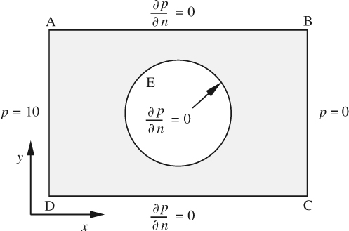
Fig. 14.1 Region and its boundary conditions, extending any distance normal to the plane of the figure.
The pressure is governed by d’Arcy’s equation:
Note that Problem 14.2 requests a modification, in which the circular region has a higher permeability, with κ = 5.
Solution
1. Load COMSOL
The loading of COMSOL will vary from one installation to the next, so local procedures must be consulted. For the earlier FEMLAB 2.3 on the author’s Macintosh G4 computer, MATLAB must first be loaded, and then "femlab" is typed at the prompt. For FEMLAB 3, used for all the examples in this book, only the FEMLAB icon needs to be clicked for both the Macintosh and PC versions. The program produces extremely similar results for both types of computers—compare, for example, the Model Navigator windows in Figs. 14.2(a) (PC) and 14.2(b) (Macintosh), whose formats are virtually identical, except for minor details such as the reversal of the order of the OK and Cancel buttons in the lower right-hand corners. This chapter is generally illustrated by Macintosh screen captures, except for the very similar PC windows shown in Figs. 14.2(a) and 14.16(b).

Fig. 14.2(a) The model navigator window—PC version, showing the options available after selecting “New,” “Chemical Engineering Module,” “Momentum balance” and “Darcy’s law.”

Fig. 14.2(b) The model navigator window—Macintosh version, after the same selections as in Fig. 14.2(a).
2. Model Navigator
After COMSOL is loaded, the foremost window is the Model Navigator. Fig. 14.2(b) shows its appearance on a Macintosh computer after the following steps:
(a) Make sure the space dimension is set to 2D, but also note the other available options.
(b) Under the New tab:
• Double-click Chemical Engineering Module.
• Double-click Momentum balance.
• Double-click Darcy’s law.
You will now see the COMSOL or FEMLAB graphical interface (Fig. 14.3) ready for you to enter the details of the problem to be solved.

In the graphical interface, take a minute to examine the menu bar and the main toolbar buttons at the top of the screen (Fig. 14.4/a/b/c/d) and the draw toolbar buttons at the left of the screen (Fig. 14.7). The menu bar consists of 11 pulldown menus (ten for a PC, which lacks the COMSOL or FEMLAB pulldown), each of which has a few or several options. A typical FEMLAB solution involves most—but not usually all—of these pulldown menus, proceeding from left to right. The toolbar buttons at the top of the graphical interface offer a quick duplication of the more common pulldown menu items. Similarly, the draw toolbar buttons offer a convenient alternative to several of the items (drawing a circle, for example) that appear in the Draw pulldown menu.


3. Options
(a) Pull down the Options menu to Axes/Grid Settings.
(b) Under the Axis option (Fig. 14.5):
• Set x min and x max to –1.5 and 1.5, respectively.
• Set y min and y max to –1 and 1, respectively.

Fig. 14.5 The axes-settings dialog box. For the PC, the positions of the “Apply” and “OK” buttons are reversed.
(c) Under the Grid option (Fig. 14.6):
• Clear Auto.
• Set x spacing and y spacing to 0.25 and 0.1, respectively.
• Click OK.

Fig. 14.6 The grid-settings dialog box. For the PC, the positions of the “Apply” and “OK” buttons are reversed.
4. Draw
(a) Either pull down the Draw menu to Draw Objects and thence to Rectangle/Square or click once on the corresponding button at the top of the column on the left of your screen. (Before you click, but with the cursor moved to this or any other button, you will soon see a notice telling you the function of the button.)
• Draw a rectangle with two of its opposite corners having coordinates (–1.25, 0.8) and (1.25, –0.8). Note that this rectangle will automatically be labeled R1. It also appears in pink, indicating it is the (only) currently selected object.
(b) Either pull down the Draw menu to Ellipse/Circle (Centered) or click once on the corresponding button near the top of the column on the left of your screen.
• Hold down the Control key (this will insure you get a circle and not an ellipse) and draw a circle of radius 0.5 centered at (0,0). The x/y coordinates of the cursor position are shown in the window at the bottom left corner. As you draw the circle, this window will also indicate its radius. Note that this circle will automatically be labeled C1. It also appears in pink, whereas the rectangle R1 is now gray.
(c) Pull down Edit to Select All, and note that R1 and C1 are now both pink. The same result can be achieved by clicking the mouse with the cursor at the top left of the screen and dragging it to the lower right, thus encompassing both R1 and C1 with a dotted rectangle.

Fig. 14.7 The left column of draw toolbar buttons. The right column (not shown above) is not needed for introductory work.
(d) Either pull down the Draw menu to Create Composite Object or click once on the corresponding button, which is sixth from the bottom in the column on the left of your screen. See Fig. 14.8.
• In the Set formula window, type R1-C1, in which “-” is the set difference operator. Ignore Keep interior boundaries at present.
• Click OK, and note that the single region (a rectangle with a hole in it) is now labeled CO1 (Fig. 14.9).


Fig. 14.9 The graphical user interface with the composite rectangle/hole region. At the bottom left there is a message log just above the status bar.
Drawn objects can be selected, moved, rotated, and deleted, etc., as with most other drawing programs. Note that each object drawn is automatically assigned a name and a label, such as R1 for the first rectangle or E2 for the second ellipse. To determine precise information about an object—such as the coordinates of the corners of a rectangle, or of the center of a circle, double-click on the object while in Draw mode; a dialog box will open with all pertinent information. If you wish, you can change any of the object’s geometric parameters (independently of the prevailing grid) or even its name.
5. Boundary
Pull down the Physics menu to Boundary Settings. Highlight each of the eight boundary segments in turn in the Boundary selection box (see Fig. 14.11) and use either the Pressure condition or Insulation/Symmetry to establish the following boundary conditions:
• Pressure p = 10 on the left-hand (inlet) edge AD of the rectangle.
• Pressure p = 0 on the right-hand (exit) edge BC of the rectangle.
• Insulated boundary conditions n · u = 0 on the remaining six boundary segments.
Note that as each segment is selected inside the Domain selection box, the corresponding boundary in the drawing behind it (Fig. 14.10) is highlighted in red. For example, AD is segment 1, etc. Also, several segments having the same boundary condition (notably 5–6–7–8 around the hole) can be highlighted simultaneously by first holding down the Shift or Command key (Control key for a PC) and then clicking on each in turn.


Fig. 14.11 The boundary-settings dialog box. For the PC, the positions of the “Apply” and “OK” buttons are reversed.
Pull down the Physics menu to Subdomain Settings, and observe that the region is currently transparent.
• In the subdomain-settings dialog box (Fig. 14.12), select subdomain 1 (the only one we have) and observe that the region becomes pink. The window also shows that the equation ∇· (–κ/η∇p) = F is being solved.
• Set the permeability κ = 1 and the viscosity η = 1, with the generation term F = 0. Ignore the time-scaling coefficient.
• Click OK.
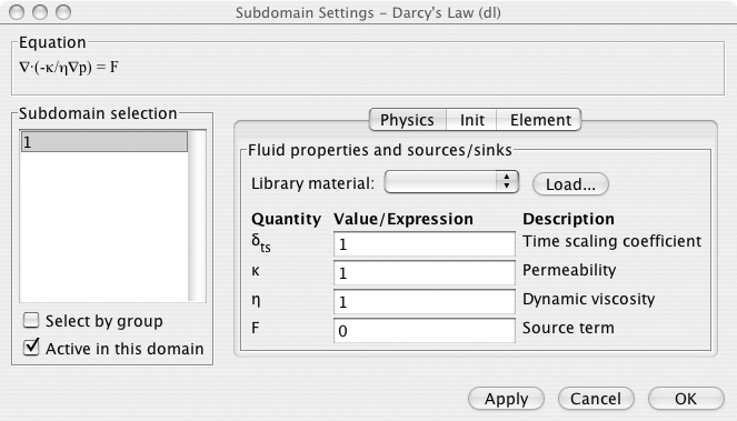
Fig. 14.12 The subdomain-settings dialog box. For the PC, the positions of the “Apply” and “OK” buttons are reversed.
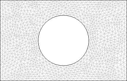
7. Mesh
• The mesh for the finite-element solution is generated automatically by pulling down the Mesh menu to Initialize Mesh. You will see many triangular elements and can find out exactly how many by pulling down to Mesh Statistics; the number of degrees of freedom tells you how many unknowns (both velocities and pressures in the case of the Navier-Stokes equations) exist in the simultaneous equations that are about to be solved.
• Also pull down the Mesh menu to Refine Mesh, as in Fig. 14.13, which would be particularly desirable for solving problems whose geometry is more complicated than in the present case.
Pull down the Solve menu to Solve Problem, which will effect the solution of the simultaneous equations generated by the finite-element method. The results then appear in a 2D Surface plot as the velocity field. However, we want the pressure field, so pull down the Postprocessing menu to Plot Parameters; select the Surface option, and adjust Predefined quantities to Pressure. After OK, you will obtain Fig. 14.14, in which the pressure varies from high (red) at the left to low (blue) at the right, with symmetry about the x axis (y = 0).

Fig. 14.14 Two-dimensional surface plot. In color, there is a progression from red (high pressure) at the left to blue (low pressure) at the right.
9. Postprocessing
Now that the finite-element method solution is complete, the results may be displayed in several different ways. Quick Plots gives rapid results, but without complete control, for example:
• Verify the nature of the plot just generated by pulling down the Postprocessing menu to Quick Plots and thence to 2D Surface Plot and observe that nothing changes.
• 3D Surface plot. By “grabbing” the base of the “box” you can rotate the plot to any desired position.
For complete control of the plots, select Postprocessing, Plot Parameters, and the General tab, as in Fig. 14.16(b), which allows you to check exactly those plot(s) you want, for example:
• After checking Contour under the General tab, select pressure under the Contour tab (Fig. 14.16(a)), click OK and observe the isobars (contours of equal pressure) in Fig. 14.15. Note that the default case is 20 contours.
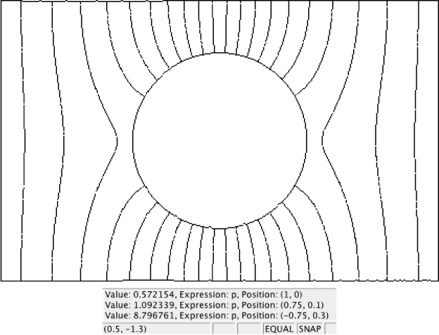
Fig. 14.15 Isobars. A forthcoming version of COMSOL will allow labeling of the isobars with the values of the pressure.

Fig. 14.16(a) The Plot Parameters dialog box with the contour tab selected—Macintosh version. Note that 20 pressure contours (isobars) are requested. For the PC, the positions of the “Apply” and “OK” buttons are reversed. A click on the arrow at upper right leads to “Deform” and “Animate” options.

Fig. 14.16(b) The Plot Parameters dialog box with the general tab selected—PC version. Note that a surface plot is requested.
• Again under the Contour tab, reduce the number of levels to 10 and change the color uniformly to black. Click OK and observe the results.
• Arrow plot gives arrows that indicate the flow direction, with the velocities proportional to the lengths of the arrows (Fig. 14.17, with contours).

Fig. 14.17 Two plots have been requested—contours (without labels) and arrows (showing the streamlines).
• Streamline plot shows the paths taken by the fluid.
• Try another contour plot, but now change Predefined quantities to Pressure gradient, ∇p, click OK and observe the results.
Note that there are many other options—explore them!
• To save your work at any stage in a file, pull down the File menu to Save and enter a name for the file. There are two formats (in FEMLAB 3): FEMLAB Model File (*.fl), and Model M-file (*.m), the latter for use with MATLAB only. FEMLAB 2.3 uses Model MAT Files (*.mat).
• To leave COMSOL pull down COMSOL to Quit COMSOL (for a PC, File to Exit or click on the cross in the upper right-hand corner).
• Perform any log-out procedure, as appropriate. Next time, try the toolbar buttons and/or keystrokes instead of the pulldown menus.
14.3. Draw Mode
The various modes can be activated either by pulling down the appropriate menu from the menu bar at the top of the screen or by clicking on one of the main toolbar buttons immediately below (see Fig. 14.4(a)).
The draw-mode toolbar buttons are shown in Figs. 14.18, 14.21, 14.22, and 14.23, which are segmented repeats of Fig. 14.7. Those shown in Fig. 14.18—for drawing various shapes and lines—are almost self-explanatory, except that the last two need a little more explanation.


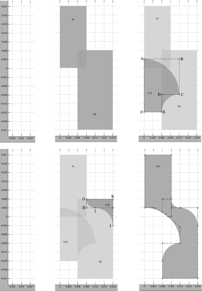
Fig. 14.20 Four stages in the development of a composite object using the “draw arc” (2nd-degree Bézier curve) tool; (a) and (b) are at top, (c) and (d) below.


1. Draw 2nd-degree Bézier Curve (“Arc” for short)
We wish to draw the region depicted in Fig. 14.19, which is needed in Example 11.3 for solving non-Newtonian flow in an extrusion die. Referring to Fig. 14.20(a), start with the two rectangles R1 and R2.1 Then, as in Fig. 14.20(b), select the Draw “arc” tool and click on points A, B, and C to draw an elliptical arc, tangential to AB and BC, that is a quarter of an ellipse with semiaxes equal to AB and BC. If AB = BC, the arc will be circular.
1 Fig. 14.20 was actually drawn in FEMLAB 2.3, but the same result is also achieved with FEMLAB 3.
Continue by clicking on two additional points, D and E, still with the Draw “arc” tool selected. Select the Draw line tool before clicking on the last point F. To stop drawing and fill-in to give the pink-shaded composite object CO1, click on any drawing tool (such as a rectangle) except a line or either of the Bézier curves (or right-click anywhere on a PC). Use a similar procedure to generate the second composite object CO2, as in Fig. 14.20(c). Finally, as in Fig. 14.8, open the Create Composite Object window, and enter R1+R2-CO1-CO2 in the Set formula window to give the single desired final object, now labeled CO1, shown in Fig. 14.20(d).
A cubic or 3rd-degree Bézier curve is determined by clicking on four points in sequence, and permits more control of its shape than does an elliptical or circular arc. After such a curve has been generated, it may be reshaped either by grabbing and moving any of its four “vertex” points, or by pulling down the Draw menu, selecting Object Properties, and entering the desired new information. When filled in, the object may be moved either by grabbing it and relocating to the desired new position, or by selecting the object and using the Move tool to specify the extent of movement in the two coordinate directions.
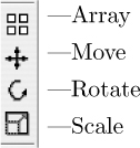
3. Array/Move/Rotate/Scale—Fig. 14.21
After an object has been selected, Array enables it to be repeated and moved any number of times in the x and y directions. Selection of the Move tool opens a window in which the desired object displacements in the x and/or y directions can be entered. Similarly, the Rotate tool opens a window asking for the desired rotation angle in degrees and the x and y coordinates of the center of rotation.
The Scale tool window asks for x and y scale factors and the corresponding base coordinates; the selected object will be expanded or contracted by the factors entered for the two coordinate directions, relative to the base coordinates.
4. Boolean Operations—Fig. 14.22
Consider two objects “A” and “B” that have been drawn and have a common region in which they overlap each other. Now select both of them, either by using the cursor to outline a rectangle that includes both of them, or by pulling down the Edit menu to Select all, or by using the Control–A combination.
The Union tool will give an object that includes both A and B. The Intersection tool will give the region that is common to both A and B. And the Difference tool will create a region in which A has deleted from it that region in which it is overlapped by B.
5. Miscellaneous Operations—Fig. 14.23
The Create composite object tool opens a window whose use has already been illustrated. It also displays two radio buttons that allow shortcuts for the Union and Intersection operations just described above.
The Create composite object window also displays another button—Keep interior boundaries. To explain, consider the composite object CO1 formed from a rectangle R1 and an ellipse E1, either by typing R1+E1 in the Set formula window or by using the Union shortcut. The result is shown in Fig. 14.24a, whether or not the Keep interior boundaries button is activated. However, when setting the differential equation coefficients later in the Subdomain mode, there will be a difference, as follows:
1. If the Keep interior boundaries button is not activated, the appearance will be similar to that in Fig. 14.24(a), except that there will be a single continuous border around the whole composite object.
2. If, however, the Keep interior boundaries is activated, the appearance will be that in Fig. 14.24(b). Although there is still one object, it is now subdivided in this example into three subdomains, which we have labeled as A, B, and C. (Region A has been selected and will appear in pink on the screen, with B and C in gray.) Such an arrangement may be advantageous because it allows different physical properties to be assigned to each of these subdomains.

Fig. 14.24 (a) Composite object formed from the union of a rectangle and an ellipse. In (b), the letters A, B, C have been added later. See the text for an explanation.
The Split button can be used on a composite object. Consider for example the composite object CO1 in Fig. 14.24(a). When it is selected and the Split button activated, its three subregions (A, B, and C in Fig. 14.24(b)) will be labeled O1, O2, and O3, each of which can be selected and moved around, as in Fig. 14.25. With some imagination and practice, unusual shapes can readily be created.

Fig. 14.25 After the “split” operation, a composite object such as that in Fig. 14.24(a) can be dissected into its component parts, each of which can then be moved independently of the others.
If we have an object whose area is shaded (as is normal), the Coerce to curve button will yield just the boundary of the object, and the Coerce to solid button will have the reverse effect, filling in a boundary. Finally, Fillet (see Example 12.5) enables a selected corner to be rounded to a specified radius, and Chamfer cuts off the corner to a specified distance.
14.4. Solution and Related Modes
The following steps are needed to solve the problem at hand. Most of the basic ideas have been adequately covered in Example 14.1 and will not be repeated here. Only a few extra points will be mentioned. Most of the operations can be achieved either through the toolbar buttons or by the more comprehensive pulldown menus.
Setting the boundary conditions. The boundary conditions will vary with the type of problem being solved. COMSOL can accommodate all boundary conditions of physical significance. Also, if the dependent variable were to vary along a boundary as, for example, u = 10 sin[5(x – 0.5)], where x is the horizontal coordinate, then the arithmetic expression 10*sin(5*(x - 0.5)) would be entered into the appropriate window, the understanding being that arguments for the trigonometric functions are in radians.
Inserting equation coefficients. As indicated in Fig. 14.12, the dialog box for the subdomain settings provides the opportunity for setting the values of the various coefficients in the PDE. Again, these values can be specified as functions of position if desired.
Establishing the finite-element mesh. The Initialize Mesh option is usually activated to start the mesh generation, followed by as many applications of Refine Mesh as are needed to obtain the desired accuracy. In practice, just one application of Refine Mesh will suffice for most problems. Also, if extra definition is needed in one part of the region, activation of Refine Selection followed by dragging the cursor over a region will generate more and finer finite elements in that region.
Solving the simultaneous equations. Activation of Solve Problem then solves the simultaneous equations generated by the finite-element method. Clearly, the more elements that are created, the longer is the time needed for the solution. The progress of the solution is automatically indicated by a window that displays how far the solution has progressed, with messages such as “LU factorization,” “Assembling,” and “Solving linear equations,” which are mainly of significance to those interested in numerical methods.
Examining the results. There is a multitude of ways in which the results can be displayed. The most important of these have already been introduced in Part 9, “Postprocessing,” of Example 14.1, and will not be repeated here. The user should gain experience by experimenting with many of the various options. COMSOL also allows the opportunity for “zooming” in (and out) to vary the magnification of the displayed results. Also, the Zoom Extents button is very useful—it will give an image that automatically fills the screen as much as possible.
14.5. Fluid Mechanics Problems Solvable by COMSOL
This section lists seven general types of fluid-mechanics problems that can be solved by COMSOL. The software is exceptionally versatile and can also solve multiphysics problems with, e.g., combined heat and mass transfer, fluid mechanics and electromagnetics—as illustrated for electroosmosis in Examples 12.4 and 12.5.
In their appearance the following equations parallel those in the FEMLAB manuals cited earlier, although slight changes have occasionally been made to conform to the notation in this book. The equations have been left in vector form, the understanding being that COMSOL will automatically reformat them according to the number of dimensions and the coordinate system specified by the user.
1. Navier-Stokes Equations
The governing equations for incompressible flow are the momentum balance and continuity equation:

Although the body-force vector F per unit volume usually accounts for gravitational attraction, it could also be the force on a charged particle in an electric field (see Examples 12.4 and 12.5). Further, if the energy equation is being solved simultaneously for temperature, F can account for free convection if temperature-dependent density variations are accommodated.
Boundary conditions. COMSOL can accommodate any or all of the following boundary conditions, each corresponding to a practical physical situation. As usual, n is the unit vector in the outwards normal direction.
No slip
Specified velocity with normal component v0
Slip or symmetry (no normal velocity component)
Specified pressure p0
“Straight-out” condition—zero tangential velocity and zero pressure
Neutral—no transport by shear stress
2. Turbulent-Flow Equations
Here, v is the time-averaged velocity, k is the turbulent kinetic energy per unit mass, and ε is the rate of dissipation of this energy. The first two equations are the momentum balance and continuity equation (Cμk2/σkε is the same as νT in Eqn. (9.90a) since σk = 1), followed by equations for the rate of growth of k and ε:


In the above, the model constants are
Wall boundary conditions. COMSOL can accommodate most of the boundary conditions listed under the Navier-Stokes equations above—with one major exception. Namely, because there are extremely sharp velocity gradients in the very thin region next to a wall, it is quite impractical to use a small enough mesh to accommodate such gradients accurately. Therefore, we lean on the knowledge that the velocity profile is logarithmic near the wall (but not all the way up to the wall), and set the following conditions close to the boundary, in which v is the velocity component parallel to the wall, n is the normal distance from the wall, ν is the kinematic viscosity, κ ![]() 0.42, and C
0.42, and C ![]() 5 for smooth walls.
5 for smooth walls.
Velocity parallel to a wall

Turbulent energy

Turbulent dissipation
3. Laplace and Poisson Equations
COMSOL is capable of solving many “classical” types of partial differential equations. Of these, the following two will be useful when solving irrotational (inviscid) flow problems.
Poisson’s equation
In the last equation c is essentially a conductivity and f is a source or generation term; both c and f may be functions of position. The corresponding boundary conditions are either of the Dirichlet type (u specified) or of the Neumann type (involving the normal derivative n. ∇u = ∂u/∂n).
4. Non-Newtonian Flows
The momentum and mass balances are the same as for the Navier-Stokes equations for Newtonian flows except that η is used instead of μ for the viscosity.

The variety of available boundary conditions is the same as for the Navier-Stokes equations. Two models are available for the non-Newtonian viscosity η, in which the strain rate ![]() (also known as the shear rate) is automatically computed by COMSOL as a function of the several velocity gradients as in Eqn. (11.10):
(also known as the shear rate) is automatically computed by COMSOL as a function of the several velocity gradients as in Eqn. (11.10):
Power-law model
Here, κ is the consistency index and n is the power-law index.
Carreau model
Here, η0 and η∞ are the viscosities at zero and very high strain rates, respectively, θ is a relaxation time of the fluid, and n is a dimensionless constant approximately in the range 0.2–0.5 for many polymer melts.
5. Flow in a Porous Medium
Incompressible flow in a porous medium is governed by the continuity equation, ∇ · v = 0, which, when coupled with d’Arcy’s law, v = –(κ/μ)∇p, gives:
For compressible flow, the continuity equation is ∇ · ρv = 0, so the governing equation now includes the variable density:
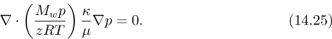
In the important case of underground storage of natural gas of molecular weight Mw and compressibility factor z at an absolute temperature T, Eqn. (14.24) becomes:
Boundary conditions. There are three relevant types of boundary conditions, in which n is the unit outward normal:
Specified pressure p0
Impervious (no flow) boundary or plane of symmetry
Specified superficial velocity u0 in the outward normal direction
6. Induced Flow in a Porous Medium—the Brinkman Equation
Some problems involve a porous medium in contact with an “open” region in which flow is unimpeded by such a porous medium; such conditions prevail for flow in the vicinity of porous catalysts and in fuel cells. In this event, there is a shear-stress induced flow in the porous medium, where the situation is governed by the Brinkman equations:
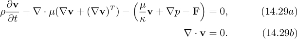
In the “open” region, the usual Navier-Stokes equations govern the viscous flow. By selecting the Brinkman option, such problems can be solved by COMSOL. The F term can accommodate mild compressibility effects.
7. Compressible Inviscid Flows
The continuity, momentum, and energy equations are:
in which the dyadic product vv is defined in Appendix C, e is the total (potential plus kinetic) energy per unit volume, F is a body force per unit volume, and Q is a heat generation per unit volume. Three additional equations are needed, assuming ideal gas behavior. First, the pressure is calculated from:

in which γ = cp/cv is the ratio of specific heats. Second, the speed of sound is obtained from Eqn. (3.80):

Third, the Mach number is needed because it determines how the boundary conditions are handled:
For subsonic flow (M < 1), the density, velocity, and pressure are specified at both the inlet and outlet, and a slip condition is applied at solid boundaries.
For supersonic flow (M > 1) the same conditions will hold at the inlet and solid boundaries, but the outlet is governed by a neutral boundary condition, which does not add any constraints to the flow.
Problems for Chapter 14
There are only two problems here, but completion of both of them will reinforce many of the fundamentals of COMSOL. For additional practice the reader is encouraged to read the several COMSOL examples throughout the book, also perhaps duplicating or modifying them. Nothing succeeds like constant practice!
1. Introductory check. Repeat the steps in Example 14.1, and make five representative prints, corresponding to Figs. 14.9, 14.13, 14.14, 14.15, and 14.17.
2. Central conductive hole. Also solve the problem in Example 14.1, except that the central circular region now has a permeability of κ = 5. Note that you no longer need to consider the internal interface between the circle C1 and rectangle R1, which is automatically accommodated by COMSOL. When you open the Create Composite Object dialog box, you will now need to:
• In the Set formula window, type R1+C1, in which “+” is the set union operator. (If ever needed, “*” is the set intersection operator.)
• Make sure the Keep interior boundaries box is checked.
Make two additional prints for this second problem, analogous to Figs. 14.15 and 14.17.